
An Intelligent Time-Series Model for Forecasting Bus Passengers Based on Smartcard Data


Abstract
:1. Introduction
- (1)
- To identify the important attributes that affect passenger flow from a total of 42 attributes in the smartcard system;
- (2)
- To add other variables that affect passenger flow, such as climate, time, space, and lag period, to establish a prediction model;
- (3)
- To apply multilayer perceptron (MLP), support vector regression (SVR), radial basis function (RBF) neural network, and long short-term memory network (LSTM) methods to forecast passenger flow with different types of time data series (weeks, weekdays, and holidays);
- (4)
- To propose an integrated-weight time-series forecast model that uses forecast data from the top three of the 80 intelligent forecast models as the adaptive factors;
- (5)
- To provide results that can be used as a reference by the government, industry, and related personnel.
2. Literature Review
2.1. Forecasting Passenger Flow by Smartcard Data
2.2. Time Series Forecasting
2.3. Intelligent Forecast Methods
- (1)
- Support vector regression (SVR)
- (2)
- Multilayer perceptron neural network (MLP)
- (3)
- Radial basis function (RBF) network
- (4)
- Long Short-Term Memory (LSTM)
3. Proposed Model
- Passenger flow forecasting is a periodic pattern, and many forecast models have been proposed to address this pattern. Previous studies have shown that datasets of no more than one month can be used to predict passenger flow at intervals of 5 or 15 min, and some studies use longer time datasets to predict passenger flow, such as daily or weekly intervals. To avoid the impact of extreme passenger flow, some studies do not consider the data collected on national holidays or weekends, and some studies treat special data as another forecast model for separate training. There is some room for improvement to obtain satisfactory results.
- To solve the shortcomings of the model, more and more studies are taking advantage of different methods that complement each other and proposing hybrid models to forecast passenger flow. These hybrid models mainly combine traditional algorithms and neural networks, but their nature still has limitations. Hence, hybrid models can be further strengthened to obtain the dynamics and forecasts of passenger flow.
- Most research in this area has focused on passenger flow forecasting for railways, high-speed railways, and subways. Compared with other public transportation systems, there have been fewer studies forecasting bus passenger flow based on smartcard data, and few studies have considered time-series lag periods as forecast variables.
- Previous research on the spatio–temporal nature of smartcard data has been widely conducted, and different attributes have been used in these studies; however, these studies have rarely discussed why these attributes have been selected and which attributes should be used in these methods. The selection and combination of input attributes is an important bridge between methods and forecast results.
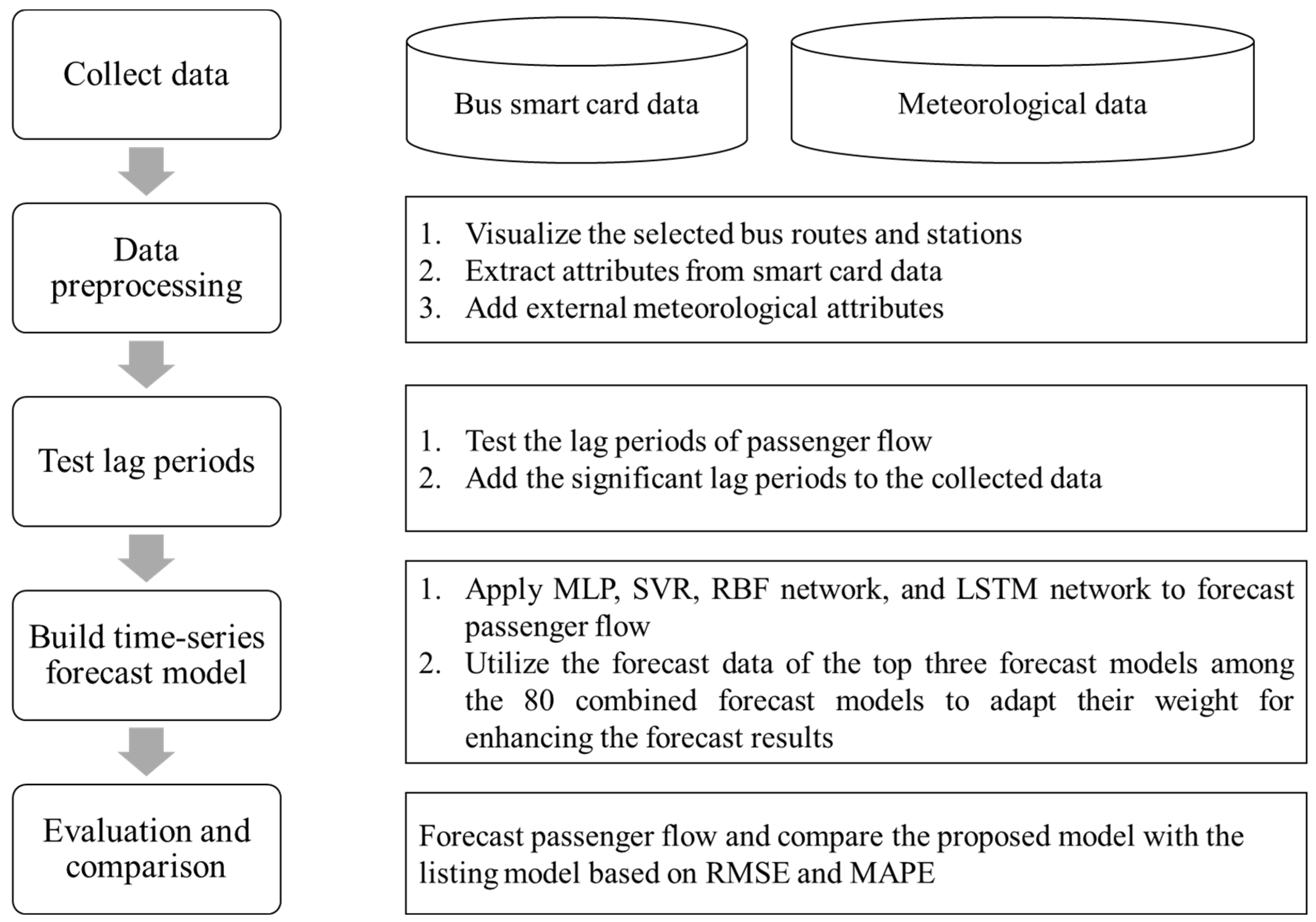
- Computational steps
- Step 1: Data collection
- (1)
- One type was smartcard data from a bus industry in Kaohsiung City, Taiwan; the data were collected over a total of 669 days, including 2,865,763 records from January 2018 to October 2019, 17 bus lines (routes), and 137 bus stations. There were 42 attributes in the collected data (see Table 1), covering 15 administrative districts of Kaohsiung City in Taiwan. Regarding data location, the longitude range is 22.58706 to 22.792377, and the latitude range is 120.32016 to 120.29944.
- (2)
- The other data type was meteorological data because the number of passengers boarding is often affected by many external factors, especially weather, which has always affected the travel behavior of passengers. Many researchers have presented the impact of weather conditions on passenger flow [13,14,15]. We collected weather data from the Kaohsiung Meteorological Bureau.
- Step 2: Data preprocessing
- Step 2.1: Extraction of attributes from smartcard data
- Step 2.2: Addition of external meteorological attributes
- Step 3: Test lag periods
- Step 4: Establishment of an integrated-weight time-series forecasting model
- F(t) is the forecast of the number of passengers at time t,
- T(t − 1) denotes the actual number of passengers at time (t − 1),
- first(t) represents the forecast of the best model for the number of passengers at time t,
- second(t) is the forecast of the second-best model for the number of passengers at time t,
- third(t) denotes the forecast of the third-best model for the number of passengers at time t,
- α is the parameter of first(t),
- β represents the parameter of second(t),
- γ denotes the parameter of third(t), and the range of α, β, and γ is from −1 to 1 (−1 means a negative correlation, and 1 represents a positive correlation).
- Step 5: Evaluation and comparison
4. Experimental Comparison
4.1. Experimental Results
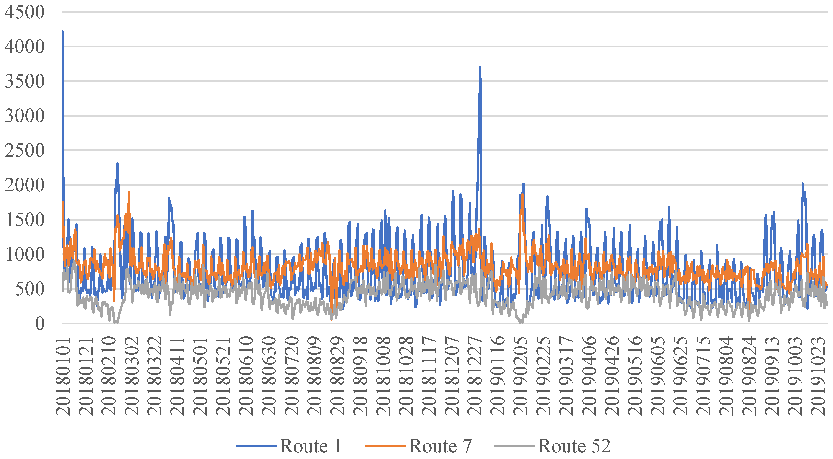
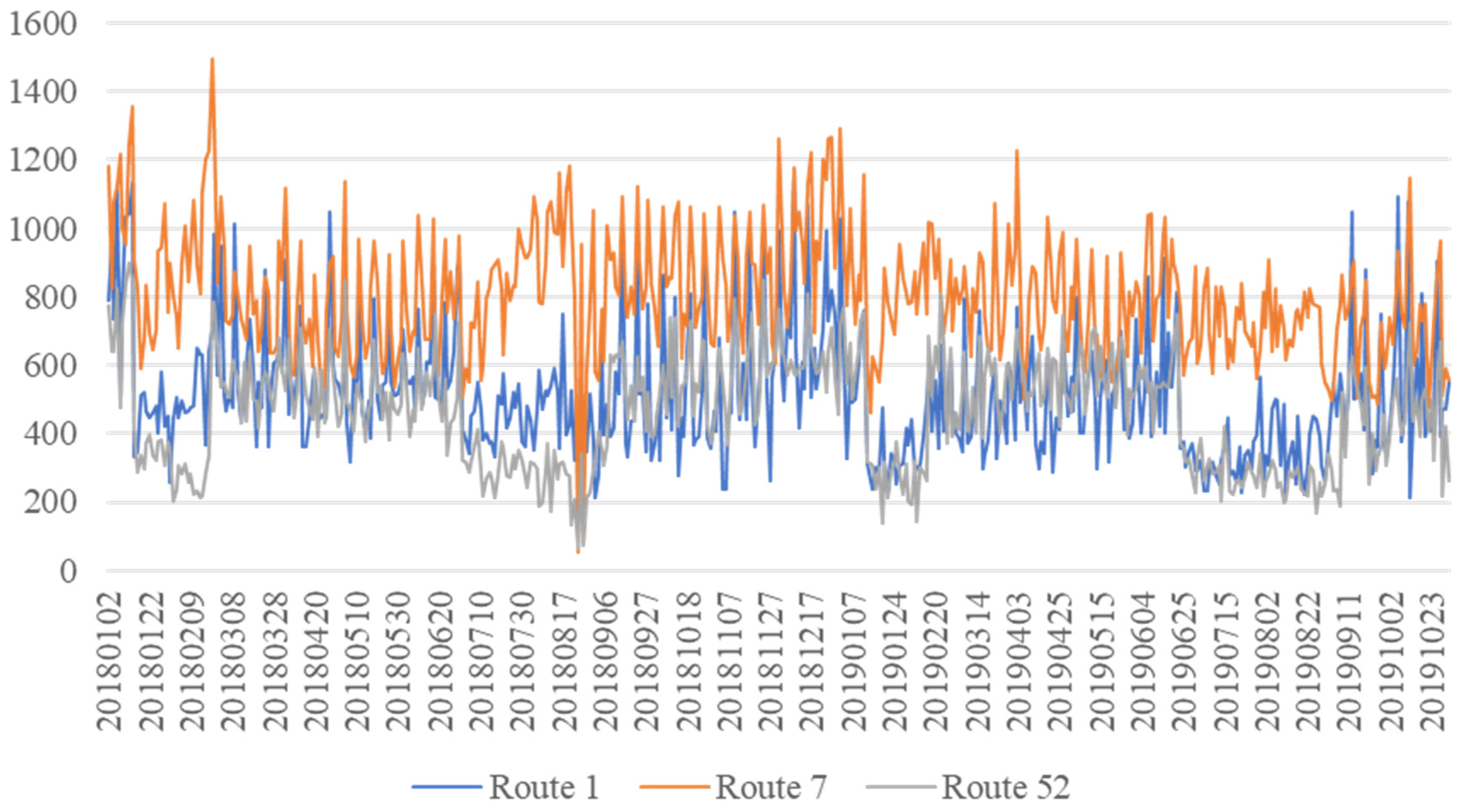
- (1)
- Route 1
- (2)
- Route 7
- (3)
- Route 52
4.2. Findings and Discussion
- (1)
- Key attributes
- (2)
- Lag period
- (3)
- Model performance
- (4)
- Sensitivity analysis
5. Conclusions
- (1)
- We proposed an integrated-weight time-series forecast model to forecast passenger flow. We used real smartcard data to verify that the proposed model has good predictive capabilities, rather than using simulated data to show the research results. The experiments showed that the proposed model performed better than the listed models for each route for different time series, as shown in Table 6, Table 7 and Table 8.
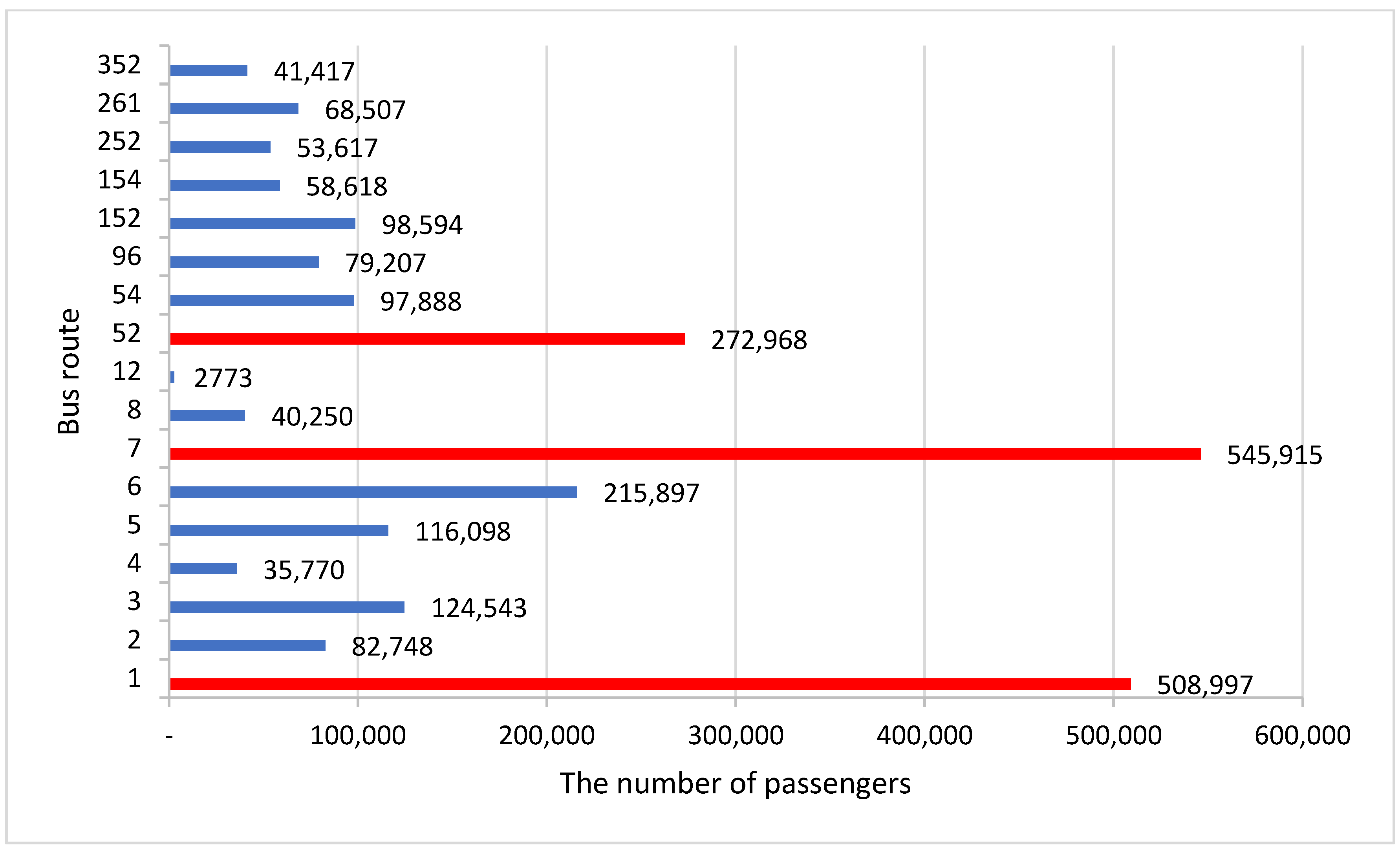
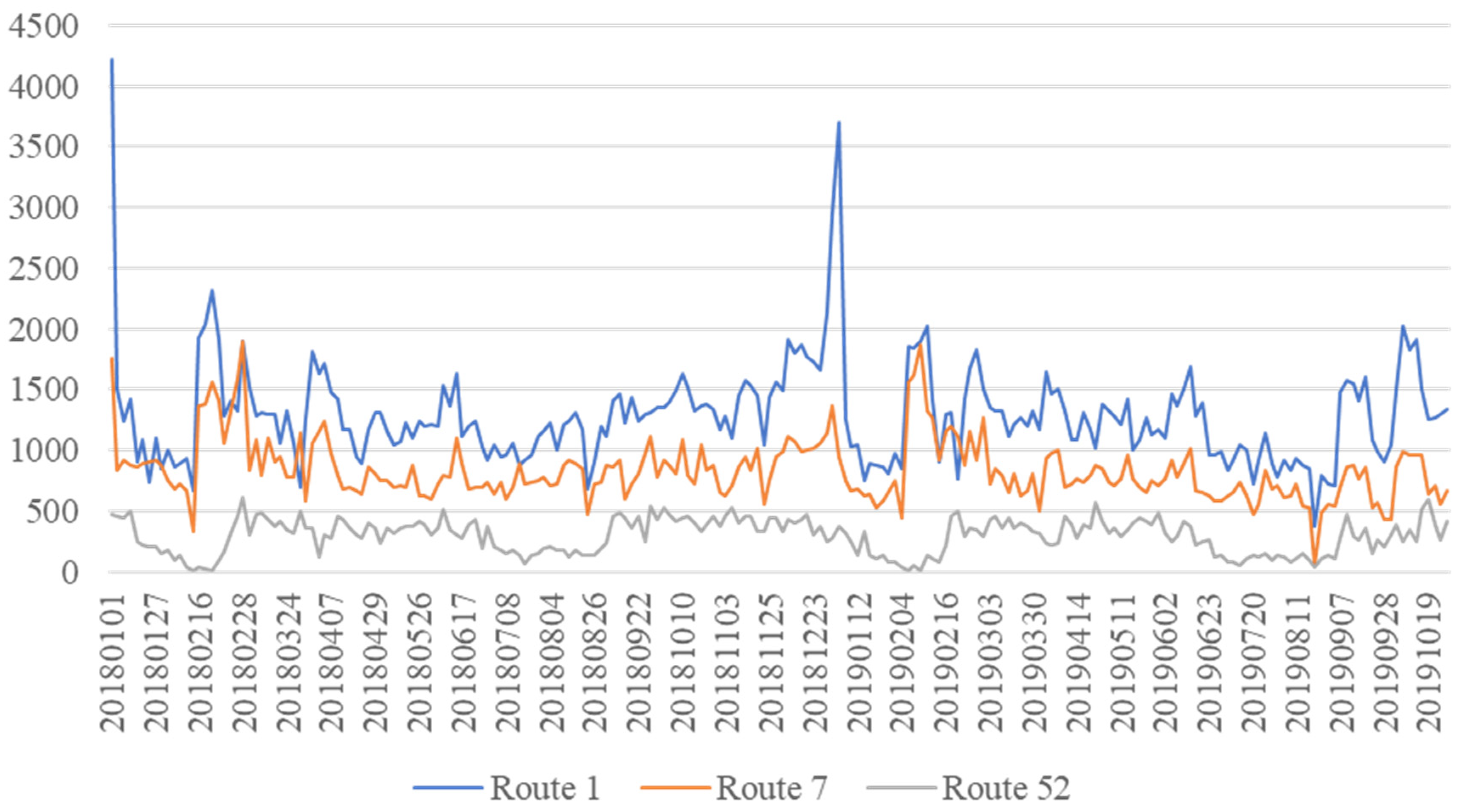
- (2)
- In terms of the verification data, we focused on the top three routes with the most passengers out of the 17 routes—Route 1, which showed the largest fluctuations; Route 7, which has the largest number of passengers; and Route 52, which has the least number of passengers of the top three routes—as shown in Figure 2.
- (3)
- In terms of attribute screening, this study used smartcard data and time attributes as well as 15 external weather attributes. In addition, as the number of passengers varies with time, this is a time-series forecasting problem; hence, seasonal trends had to be considered. Therefore, we added the number of lags to the forecast of passenger flow.
- (4)
- As shown in Table 6, Table 7 and Table 8, we found that the data for each route could be partitioned by time (weeks, weekdays, and holidays) to improve the forecast result. Based on the key attributes shown in Table 9 and the lag periods of the top three models shown in Table 10, the number of lags affected forecast results. Furthermore, most of the top three models are in the LSTM family, which presents a better forecast.
Author Contributions
Funding
Institutional Review Board Statement
Informed Consent Statement
Data Availability Statement
Acknowledgments
Conflicts of Interest
References
- FTA. Transit’s Role in Environmental Sustainability. 2015. Available online: https://www.transit.dot.gov/regulations-and-guidance/environmental-programs/transit-environmental-sustainability/transit-role (accessed on 10 August 2020).
- TMTC. Public Transport Market Share from Taiwan’s Ministry of Transportation and Communications. 2016. Available online: https://www.motc.gov.tw/uploaddowndoc?file=public/201707031545021.pdf&filedisplay=201707031545021.pdf&flag=doc (accessed on 10 August 2020).
- Trépanier, M.; Tranchant, N.; Chapleau, R. Individual trip destination estimation in a transit smart card automated fare collection system. J. Intell. Transport. Syst. 2007, 11, 1–14. [Google Scholar] [CrossRef]
- Cheon, S.H.; Lee, C.; Shin, S. Data-driven stochastic transit assignment modeling using an automatic fare collection system. Transp. Res. Part C Emerg. Technol. 2019, 98, 239–254. [Google Scholar] [CrossRef]
- Transportation Research Board. HCM 2010. Highway Capacity Manual; Transportation Research Board: Washington, DC, USA, 2010. [Google Scholar]
- Tang, T.; Liu, R.; Choudhury, C. Incorporating weather conditions and travel history in estimating the alighting bus stops from smart card data. Sustain. Cities Soc. 2020, 53, 101927. [Google Scholar] [CrossRef]
- Li, H.; Wang, Y.; Xu, X.; Qin, L.; Zhang, H. Short-term passenger flow prediction under passenger flow control using a dynamic radial basis function network. Appl. Soft Comput. 2019, 83, 105620. [Google Scholar] [CrossRef]
- Ke, J.; Zheng, H.; Yang, H.; Chen, X. Short-term forecasting of passenger demand under on-demand ride services: A spatio-temporal deep learning approach. Transp. Res. Part C Emerg. Technol. 2017, 85, 591–608. [Google Scholar] [CrossRef] [Green Version]
- Xu, S.; Chan, H.; Zhang, T. Forecasting the demand of the aviation industry using hybrid time series SARIMA-SVR approach. Transp. Res. Part E Logist. Transp. Rev. 2019, 122, 169–180. [Google Scholar] [CrossRef]
- Ma, X.; Liu, C.; Wen, H.; Wang, Y.; Wu, Y. Understanding commuting patterns using transit smart card data. J. Transp. Geogr. 2017, 58, 135–145. [Google Scholar] [CrossRef]
- Eom, J.K.; Choi, J.; Park, M.S.; Heo, T.Y. Exploring the catchment area of an urban railway station by using transit card data: Case study in Seoul. Cities 2019, 95, 102364. [Google Scholar] [CrossRef]
- Tao, S.; Corcoran, J.; Mateo-Babiano, I.; Rohde, D. Exploring Bus Rapid Transit passenger travel behaviour using big data. Appl. Geogr. 2014, 53, 90–104. [Google Scholar] [CrossRef]
- Briand, A.; Côme, E.; Trépanier, M.; Oukhellou, L. Analyzing year-to-year changes in public transport passenger behaviour using smart card data. Transp. Res. Part C Emerg. Technol. 2017, 79, 274–289. [Google Scholar] [CrossRef]
- Arana, P.; Cabezudo, S.; Peñalba, M. Influence of weather conditions on transit ridership: A statistical study using data from Smartcards. Transp. Res. Part A Policy Pract. 2014, 59, 1–12. [Google Scholar] [CrossRef]
- Tang, L.; Thakuriah, P. Ridership effects of real-time bus information system: A case study in the City of Chicago. Transp. Res. Part C Emerg. Technol. 2012, 22, 146–161. [Google Scholar] [CrossRef]
- Horowitz, R. Legal notes. J. Futures Mark. 1984, 4, 229–230. [Google Scholar] [CrossRef]
- Taylor, B.; Miller, D.; Iseki, H.; Fink, C. Nature and/or nurture? Analyzing the determinants of transit ridership across US urbanized areas. Transp. Res. Part A Policy Pract. 2009, 43, 60–77. [Google Scholar] [CrossRef] [Green Version]
- Chan, S.; Miranda-Moreno, L. A station-level ridership model for the metro network in Montreal, Quebec. Can. J. Civ. Eng. 2013, 40, 254–262. [Google Scholar] [CrossRef]
- Karlaftis, M.; Vlahogianni, E. Statistical methods versus neural networks in transportation research: Differences, similarities and some insights. Transp. Res. Part C Emerg. Technol. 2011, 19, 387–399. [Google Scholar] [CrossRef]
- Ma, Z.; Xing, J.; Mesbah, M.; Ferreira, L. Predicting short-term bus passenger demand using a pattern hybrid approach. Transp. Res. Part C Emerg. Technol. 2014, 39, 148–163. [Google Scholar] [CrossRef]
- Sun, Y.; Leng, B.; Guan, W. A novel wavelet-SVM short-time passenger flow prediction in Beijing subway system. Neurocomputing 2015, 166, 109–121. [Google Scholar] [CrossRef]
- Xie, G.; Wang, S.; Lai, K. Short-term forecasting of air passenger by using hybrid seasonal decomposition and least squares support vector regression approaches. J. Air Transp. Manag. 2014, 37, 20–26. [Google Scholar] [CrossRef]
- Liu, L.; Chen, R.C. A novel passenger flow prediction model using deep learning methods. Transp. Res. Part C Emerg. Technol. 2017, 84, 74–91. [Google Scholar] [CrossRef]
- Box, G.E.P.; Jenkins, G.M. Time Series Analysis: Forecasting and Control, revised ed.; Holden Day: San Francisco, CA, USA, 1976. [Google Scholar]
- Hou, Q.; Leng, J.; Ma, G.; Liu, W.; Cheng, Y. An adaptive hybrid model for short-term urban traffic flow prediction. Phys. A Stat. Mech. Its Appl. 2019, 527, 121065. [Google Scholar] [CrossRef]
- Wang, H.; Li, L.; Pan, P.; Wang, Y.; Jin, Y. Early warning of burst passenger flow in public transportation system. Transp. Res. Part C Emerg. Technol. 2019, 105, 580–598. [Google Scholar] [CrossRef]
- Triebe, O.; Laptev, N.P.; Rajagopal, R. AR-Net: A simple Auto-Regressive Neural Network for time-series. arXiv 2019, arXiv:1911.12436. [Google Scholar]
- Hajirahimi, Z.; Khashei, M. Weighted sequential hybrid approaches for time series forecasting. Phys. A Stat. Mech. Its Appl. 2019, 531, 121717. [Google Scholar] [CrossRef]
- Tsai, M.-C.; Cheng, C.-H.; Tsai, M.-I. A Multifactor Fuzzy Time-Series Fitting Model for Forecasting the Stock Index. Symmetry 2019, 11, 1474. [Google Scholar] [CrossRef] [Green Version]
- Jiang, Y.; Ye, Y.; Wang, Q. Study on Weighting Function of Weighted Time Series Forecasting Model in the Safety System. In Proceedings of the 2011 Asia-Pacific Power and Energy Engineering Conference, Wuhan, China, 25–28 March 2011; pp. 1–4. [Google Scholar] [CrossRef]
- Cortes, C.; Vapnik, V. Support-vector networks. Mach Learn 1995, 20, 273–297. [Google Scholar] [CrossRef]
- Castro-Neto, M.; Jeong, Y.; Jeong, M.; Han, L.D. Online-SVR for short-term traffic flow prediction under typical and atypical traffic conditions. Expert Syst. Appl. 2009, 36, 6164–6173. [Google Scholar] [CrossRef]
- Rosenblatt, F. The Perceptron—A Perceiving and Recognizing Automaton; Report 85-460-1; Cornell Aeronautical Laboratory: Buffalo, NY, USA, 1957. [Google Scholar]
- Ma, T.; Antoniou, C.; Toledo, T. Hybrid machine learning algorithm and statistical time series model for network-wide traffic forecast. Transp. Res. Part C Emerg. Technol. 2020, 111, 352–372. [Google Scholar] [CrossRef]
- Tsai, T.; Lee, C.; Wei, C. Neural network based temporal feature models for short-term railway passenger demand forecasting. Expert Syst. Appl. 2009, 36, 3728–3736. [Google Scholar] [CrossRef]
- Broomhead, D.S.; Lowe, D. Multivariable functional interpolation and adaptive networks. Complex Syst. 1988, 2, 321–355. [Google Scholar]
- Li, Y.; Wang, X.; Sun, S.; Ma, X.; Lu, G. Forecasting short-term subway passenger flow under special events scenarios using multiscale radial basis function networks. Transp. Res. Part C Emerg. Technol. 2017, 77, 306–328. [Google Scholar] [CrossRef]
- Hochreiter, S.; Schmidhuber, J. Long Short-Term Memory. Neural Comput. 1997, 9, 1735–1780. [Google Scholar] [CrossRef] [PubMed]
- Xu, C.; Ji, J.; Liu, P. The station-free sharing bike demand forecasting with a deep learning approach and large-scale datasets. Transp. Res. Part C Emerg. Technol. 2018, 95, 47–60. [Google Scholar] [CrossRef]
- Cagan, P. The monetary dynamics of hyper-inflation. In Studies in the Quantity Theory of Money; Friedman, M., Ed.; University of Chicago Press: Chicago, IL, USA, 1956. [Google Scholar]
- Kmenta, J. Elements of Econometrics, 2nd ed.; Macmillan: New York, NY, USA, 1986. [Google Scholar]
- Brockwell, P.J.; Davies, R.A. Time Series: Theory and Methods, 2nd ed.; Springer: New York, NY, USA, 1991. [Google Scholar]
- Hyndman, R.J.; Athanasopoulos, G. Forecasting: Principles and Practice, 2nd ed.; OTexts: Melbourne, Australia, 2018; Available online: https://otexts.org/fpp2/ (accessed on 15 January 2021).
- Zhang, Y.; Xiong, R.; He, H.; Pecht, M.G. Long short-term memory recurrent neural network for remaining useful life prediction of lithium-ion batteries. IEEE Trans. Veh. Technol. 2018, 67, 5695–5705. [Google Scholar] [CrossRef]
- Yang, J.; Kim, J.; Jiménez, P.A.; Sengupta, M.; Dudhia, J.; Xie, Y.; Golnas, A.; Giering, R. An efficient method to identify uncertainties of WRF-Solar variables in forecasting solar irradiance using a tangent linear sensitivity analysis. Sol. Energy 2021, 220, 509–522. [Google Scholar] [CrossRef]


| Bus schedule number | Trading time for boarding | Card payment amount for exiting |
| Station number | Types of trading | Benefit points discount for exiting |
| Station name | Voice code for boarding | Free |
| Driver number | Boarding station code | Cash |
| Driver name | Boarding station name | Penalty fine |
| Bus number | Transferring discount amount | Making up the fare difference |
| Route number | Onboard card payment amount | Company subsidy amount |
| Route name | Boarding by benefit points discount | Transaction file name for boarding |
| Card number | Trading date for exiting | Transaction file name for exiting |
| Service type | Trading time for exiting | Outbound/return |
| Trade tickets | Types of trading for exiting | Counting status |
| Fare | Voice code for exiting | Counting date |
| Smartcard payment amount | Station code for exiting | Transferring group code |
| Trading date for boarding | Station name for exiting | Smartcard company |
| Type | Attribute | Description |
|---|---|---|
| Smartcard | Month | “1” denotes Jan, “2” means Feb, …, “12” represents Dec |
| Day | “1” denotes the first day for each month, “2” means the second day for each month, …, “31” denotes the last day for each month. | |
| Week | “1” denotes Monday, “2” means Tuesday, …, “7” represents Sunday. | |
| Bus line | The attribute was applied to visualize the heat map. | |
| Bus station | The attribute was applied to visualize the heat map. | |
| Station passengers | The attribute represents the passengers boarding at each bus station, which was applied to calculate the number of passengers at all stations for each day | |
| Passengers | Number of passengers on the bus line for each day | |
| Meteorology | Temp | Average temperature, degrees Celsius, °C |
| Tmax | Maximum temperature, degrees Celsius, °C | |
| Tmin | Minimum temperature, degrees Celsius, °C | |
| RH | Relative humidity, percent % | |
| RH_min | Minimum relative humidity, percent % | |
| WS | The wind speed was taken as the average value 10 min before the observation point, meters per second (m/s). | |
| WS_max | The maximum wind speed was taken as the maximum instantaneous wind speed within 1 h before the observation point, meters per second (m/s). | |
| Precp | The precipitation was taken as the total rainfall in a day, milliliters per day. | |
| Precp_hr | Total number of rainy hours in a day, number of hours | |
| Precp_10max | Maximum precipitation within ten minutes of the day, milliliters per ten minutes. | |
| Precp_hrmax | Maximum precipitation within an hour of the day, milliliters per hour. | |
| SunS | Sunshine hours, number of hours | |
| SunS_rate | The sunshine rate is a percentage ratio of the recorded bright sunshine duration and daylight duration in a day, percent %. | |
| GloblRad | Global radiation refers to a value used to measure the solar radiation energy for a given time and area, megajoules per square meter and per day, MJ/m2. | |
| UVImax | The maximum ultraviolet index refers to the international measurement standard for the solar ultraviolet (UV) radiation intensity at a certain place on a certain day; the index value from 0 to 11+ is divided into five levels. | |
| Lag period | Lag 1 | A Lag 1 autocorrelation is the correlation between values that are one time period apart. |
| Lag 2 | a Lag k autocorrelation is a correlation between values that are k time periods apart, where k = 2, 3, 4, 5, 6, 7. | |
| Lag 3 | ||
| Lag 4 | ||
| Lag 5 | ||
| Lag 6 | ||
| Lag 7 |
| Week (Seven Days) | Weekday | Holiday | |
|---|---|---|---|
| Route 1 | Lag: 1, 2, 4, 6, 7 | Lag:1, 2, 4, 5 | Lag:1 |
| Route 7 | Lag: 1, 2, 3, 4, 7 | Lag:1, 3, 4, 5, 6 | Lag:1, 2 |
| Route 52 | Lag: 1, 2, 3, 4, 6, 7 | Lag:1, 2, 3, 4, 5 | Lag:1, 2 |
| Model Abbreviation | Full Name |
|---|---|
| MLP_1_ lin | MLP with 1 hidden layer and linear activation function |
| MLP_1_ log | MLP with 1 hidden layer and logistic activation function |
| MLP_2_ lin | MLP with 2 hidden layer and linear activation function |
| MLP_2_log | MLP with 2 hidden layer and logistic activation function |
| SVM_lin | SVR with linear kernel function |
| SVM_pol | SVR with polynomial kernel function |
| SVM_rbf | SVR with RBF kernel function |
| SVM_sig | SVR with sigmoid kernel function |
| RBF net | Radial basis function network |
| LSTM | Long short-term memory |
| Algorithm | No lag | Lag 1 | Lag 2 | Lag 3 | Lag 4 | Lag 5 | Lag 6 | Lag 7 | |
|---|---|---|---|---|---|---|---|---|---|
| LSTM | RMSE | 346.983 | 323.136 | 314.640 | 313.599 | 311.582 | 270.137 | 246.327 | 235.838 |
| MAPE | 55.297 | 51.271 | 54.108 | 53.805 | 46.663 | 42.201 | 30.713 | 29.091 | |
| MLP_1_lin | RMSE | 419.087 | 457.096 | 440.914 | 464.523 | 487.629 | 465.230 | 444.713 | 441.920 |
| MAPE | 50.414 | 40.028 | 42.689 | 39.118 | 38.048 | 39.447 | 42.019 | 42.427 | |
| MLP_1_log | RMSE | 413.770 | 422.451 | 437.535 | 442.538 | 454.443 | 413.121 | 425.137 | 473.599 |
| MAPE | 53.621 | 48.826 | 43.573 | 42.355 | 40.548 | 54.963 | 46.756 | 38.588 | |
| MLP_2_lin | RMSE | 417.011 | 436.597 | 606.395 | 496.521 | 520.526 | 451.678 | 455.457 | 481.922 |
| MAPE | 51.544 | 43.844 | 58.925 | 38.235 | 39.951 | 41.111 | 40.371 | 38.435 | |
| MLP_2_log | RMSE | 423.232 | 456.767 | 463.386 | 427.124 | 433.571 | 448.466 | 435.913 | 466.868 |
| MAPE | 48.477 | 40.148 | 39.307 | 46.883 | 44.817 | 41.475 | 43.736 | 38.926 | |
| RBF net | RMSE | 407.477 | 406.968 | 436.204 | 416.700 | 413.988 | 406.394 | 405.928 | 400.344 |
| MAPE | 67.738 | 65.773 | 44.045 | 51.765 | 54.012 | 65.769 | 64.782 | 65.439 | |
| SVR_lin | RMSE | 415.328 | 438.604 | 444.973 | 460.935 | 440.719 | 434.932 | 435.827 | 435.218 |
| MAPE | 52.564 | 43.338 | 41.875 | 39.496 | 43.074 | 45.093 | 43.985 | 43.888 | |
| SVR_pol | RMSE | 428.524 | 413.265 | 424.142 | 434.607 | 419.408 | 417.863 | 422.436 | 423.037 |
| MAPE | 46.397 | 54.061 | 41.223 | 44.322 | 50.989 | 52.713 | 49.107 | 48.805 | |
| SVR_rbf | RMSE | 437.040 | 414.256 | 422.609 | 415.376 | 419.644 | 421.224 | 420.811 | 423.770 |
| MAPE | 43.773 | 53.330 | 48.703 | 52.607 | 50.366 | 50.886 | 50.222 | 48.335 | |
| SVR_sig | RMSE | 416.775 | 445.232 | 448.546 | 446.987 | 500.864 | 441.484 | 406.373 | 410.386 |
| MAPE | 51.681 | 41.895 | 41.223 | 41.478 | 38.510 | 43.311 | 62.067 | 54.371 | |
| Week | Weekday | Holiday | ||||||
|---|---|---|---|---|---|---|---|---|
| LSTM lag 7 | RMSE | 235.838 | LSTM lag 4 | RMSE | 175.697 | LSTM lag 4 | RMSE | 255.503 |
| MAPE | 29.091 | MAPE | 34.973 | MAPE | 21.913 | |||
| LSTM lag 6 | RMSE | 246.327 | LSTM lag 1 | RMSE | 177.303 | LSTM lag 5 | RMSE | 255.907 |
| MAPE | 30.713 | MAPE | 34.003 | MAPE | 21.469 | |||
| LSTM lag 5 | RMSE | 270.137 | LSTM lag 2 | RMSE | 177.751 | LSTM lag 7 | RMSE | 259.302 |
| MAPE | 42.201 | MAPE | 36.563 | MAPE | 21.085 | |||
| Proposed | RMSE | 199.882 | Proposed method | RMSE | 115.963 | Proposed method | RMSE | 171.627 |
| MAPE | 54.534 | MAPE | 33.068 | MAPE | 20.426 | |||
| Week | Weekday | Holiday | ||||||
|---|---|---|---|---|---|---|---|---|
| LSTM (no lag) | RMSE | 142.964 | RBF net lag 4 | RMSE | 131.499 | LSTM (no lag) | RMSE | 148.165 |
| MAPE | 27.182 | MAPE | 15.400 | MAPE | 36.102 | |||
| LSTM lag 5 | RMSE | 143.360 | MLP_2_log lag 1 | RMSE | 131.794 | LSTM lag 2 | RMSE | 157.255 |
| MAPE | 27.397 | MAPE | 15.607 | MAPE | 37.800 | |||
| LSTM lag 4 | RMSE | 144.51 | MLP_2_log lag 5 | RMSE | 133.274 | LSTM lag 1 | RMSE | 164.564 |
| MAPE | 27.964 | MAPE | 15.657 | MAPE | 40.155 | |||
| Proposed | RMSE | 93.682 | Proposed method | RMSE | 82.124 | Proposed method | RMSE | 110.650 |
| MAPE | 26.728 | MAPE | 15.295 | MAPE | 35.097 | |||
| Week | Weekday | Holiday | ||||||
|---|---|---|---|---|---|---|---|---|
| LSTM lag 7 | RMSE | 117.833 | LSTM lag 1 | RMSE | 107.196 | LSTM lag 4 | RMSE | 121.741 |
| MAPE | 37.901 | MAPE | 29.631 | MAPE | 52.935 | |||
| LSTM lag 6 | RMSE | 119.873 | LSTM lag 7 | RMSE | 109.904 | LSTM lag 6 | RMSE | 121.767 |
| MAPE | 38.999 | MAPE | 28.371 | MAPE | 53.773 | |||
| LSTM lag 5 | RMSE | 131.381 | LSTM lag 2 | RMSE | 110.222 | LSTM lag 5 | RMSE | 121.943 |
| MAPE | 48.909 | MAPE | 29.768 | MAPE | 52.555 | |||
| Proposed | RMSE | 79.963 | Proposed | RMSE | 78.179 | Proposed | RMSE | 60.968 |
| MAPE | 38.126 | MAPE | 26.025 | MAPE | 41.958 | |||
| Route | Dataset | Ordering of Attribute Importance |
|---|---|---|
| Route 1 | week | Precp_10max > Precp > Precp_hrmax > lag 7 > lag 1 > Precp_hr > week > lag 5 > lag 2 > RH > month > lag 6 > Tmax > UVImax |
| weekday | Precp_10max > Precp > Precp_hrmax > Precp_hr > lag 1 > week > Temp > WS > Tmax | |
| holiday | Precp_hrmax > Precp > Precp_10max > lag 1 > Precp_hr > week > month > SunS_rate > Tmax | |
| Route 7 | week | Precp > Precp_hrmax > Precp_10max > Precp_hr > lag 1 > GloblRad > WS > RH_min > Temp > Tmin > RH > SunS_rate > UVImax |
| weekday | lag 1 > week > month > Temp > Tmin > GloblRad > Precp_hr > RH_min > Precp > Precp_10max | |
| holiday | lag 1 > week > SunS > SunS_rate > Tmin > month > GloblRad > Precp_hr > RH_min > WS > lag 2 | |
| Route 52 | week | lag 1 > week > lag 2 > SunS_rate > Tmax > GloblRad > WS_max > UVImax > Month > Precp > SunS |
| weekday | Precp > lag 1 > Precp_10max > Precp_hrmax > Precp_hr > RH > Tmin > WS_max > Day > lag 5 | |
| holiday | lag 1 > SunS_rate > lag 2 > SunS > Precp > Precp_10max > GloblRad > Tmax > Precp_hr |
| Week (Seven Days) | Weekday | Holiday | |
|---|---|---|---|
| Criteria | RMSE | RMSE | RMSE |
| Route 1 | LSTM lag 7 | LSTM lag 4 | LSTM lag 4 |
| LSTM lag 6 | LSTM lag 1 | LSTM lag 5 | |
| LSTM lag 5 | LSTM lag 2 | LSTM lag 7 | |
| Route 7 | LSTM (no lag) | RBF net lag 4 | LSTM (no lag) |
| LSTM lag 5 | MLP_2_log lag 1 | LSTM lag 2 | |
| LSTM lag 4 | MLP_2_log lag 5 | LSTM lag 1 | |
| Route 52 | LSTM lag 7 | LSTM lag 1 | LSTM lag 4 |
| LSTM lag 6 | LSTM lag 7 | LSTM lag 6 | |
| LSTM lag 5 | LSTM lag 2 | LSTM lag 5 |
| Route 1 | Route 7 | Route 52 | |
|---|---|---|---|
| Full attributes | 199.882 | 93.682 | 79.963 |
| Removal of meteorology attributes | 231.714 | 144.949 | 113.959 |
| Removal of first key attribute | 228.594 | 136.121 | 121.006 |
| Removal of second key attribute | 228.066 | 140.402 | 116.717 |
Publisher’s Note: MDPI stays neutral with regard to jurisdictional claims in published maps and institutional affiliations. |
© 2022 by the authors. Licensee MDPI, Basel, Switzerland. This article is an open access article distributed under the terms and conditions of the Creative Commons Attribution (CC BY) license (https://creativecommons.org/licenses/by/4.0/).
Share and Cite
Cheng, C.-H.; Tsai, M.-C.; Cheng, Y.-C. An Intelligent Time-Series Model for Forecasting Bus Passengers Based on Smartcard Data. Appl. Sci. 2022, 12, 4763. https://doi.org/10.3390/app12094763
Cheng C-H, Tsai M-C, Cheng Y-C. An Intelligent Time-Series Model for Forecasting Bus Passengers Based on Smartcard Data. Applied Sciences. 2022; 12(9):4763. https://doi.org/10.3390/app12094763
Chicago/Turabian StyleCheng, Ching-Hsue, Ming-Chi Tsai, and Yi-Chen Cheng. 2022. "An Intelligent Time-Series Model for Forecasting Bus Passengers Based on Smartcard Data" Applied Sciences 12, no. 9: 4763. https://doi.org/10.3390/app12094763
APA StyleCheng, C.-H., Tsai, M.-C., & Cheng, Y.-C. (2022). An Intelligent Time-Series Model for Forecasting Bus Passengers Based on Smartcard Data. Applied Sciences, 12(9), 4763. https://doi.org/10.3390/app12094763