Abstract
The urban ecosystem provides many services that help humans lead physically and mentally healthy lives. The quality of such urban ecosystem services is closely related to various urban forms, such as land cover, land use, buildings, infrastructure, population, and type and scale of green space. This study aims to promote the overall improvement and balance of an urban ecosystem’s regulating services. Initially, ecosystem regulating services are assessed according to the type of the urban space, and their contributions are analyzed based on linear regression slope and pairwise comparison of the ecosystem services. The contribution of ecosystem regulating services of Suwon City in South Korea was assessed through the following process: (1) selection of assessment indices and assessment methods for urban ecosystem regulating services; (2) urban space classification; (3) ecosystem regulating service assessment by type of urban space; and (4) pairwise comparison of ecosystem regulating services by type and for the entire study area. The study areas are classified into six type areas: forests (type A), agricultural land (type B), low-rise residential areas (type C), mid-rise mixed (residential and commercial) areas (type D), high-rise residential areas (type E), and industrial and barren land (type F). By studying representative regulating services, such as vegetation vitality, flood reduction capacity, carbon storage capacity, and heat reduction capacity, this study confirmed that type A provided the best service, while type C provided the worst. In addition, the relative contribution analysis between the regulating services based on pairwise comparison showed that the standard deviation between the contributions was 0.04 when diagnosing the entire study area, but apparently no types except type A were balanced. The reason such regulating services are imbalanced is that their vegetation vitality was calculated to be the lowest compared with the assessment indices of type A. Additionally, this imbalance was found to be most severe in the mid-rise mixed (residential and commercial) districts. Through this study, the spatial types in which the ecosystem regulating services in Suwon City are imbalanced could be determined. It was also revealed that regulating services should be prioritized for improvement in order to achieve greater balance in urban ecosystem. Such pairwise comparison results can be effectively utilized in determining the area and supply needed when formulating urban greening plans and forest restoration plans.
1. Introduction
In urban areas, where more than half of the world’s population lives, an urban ecosystem is formed in which natural and artificial spaces are intricately connected, and urban residents depend on the services provided by the ecosystem [1]. The ecosystem provides many services that help human beings lead physically and mentally healthy lives [2]. Ecosystem services (ES) are defined as the benefits [3,4] that humans obtain from nature and are mainly classified into supplying, regulating, supporting, and cultural services [2]. The quality of these urban ES is closely related to various urban forms, such as land cover, land use, buildings, infrastructure, population, location types, and scale of green areas [5,6,7,8,9]. Urban ecosystem components are more complex than those of natural ecosystems, thus even small changes can cause a chain reaction of imbalances in ES [10]. Therefore, in order to maintain a healthy cycle in an urban ecosystem, the relationships between ES should be understood in detail [11].
Numerous studies have analyzed the interrelations (trade-offs) between supplying, regulating, supporting, and cultural services, which are the most important aspects of ES [9,12,13,14,15,16,17,18]. Most of these studies emphasize the importance of harmony and balance with urban ES in increasing the benefits that human society can enjoy from urban ecosystem. In other words, sustainable conservation and maintenance of urban ecosystem is in effect possible through harmony and balance with urban ES [10]. Simultaneously, with humans recognizing the benefits of ecosystem, it becomes possible to create a virtuous cycle for ecosystem [2,19]. However, with increases in urban development and human activities, natural ecosystems are being damaged, consequently causing deterioration and imbalance in urban ES [20,21]. This causes negative effects such as reduction of animal and plant habitats, creation of urban heat islands, increased risk of flooding, and increased carbon emissions, which threaten the lives of urban residents. Such environmental problems have been mostly improved and focus on natural ecological space mainly distributed in the city without the consideration of the interrelationship between natural ecological space and humans [7,22,23]. Recently, efforts to solve these environmental problems have been increasing through socio-ecological approaches that emphasize the comprehensive interrelationship between natural ecological space and humans [24,25]. The improvement of urban natural ecological space considering the characteristics of human society can contribute to the increasing of urban ecosystem services [26]. Therefore, spatial planning, including urban planning, urban design, and landscape planning, has been applied as a major means for creating a sustainable city [27,28,29,30,31].
In the case of South Korea, various policy-initiated projects have been undertaken to improve ecosystem supplying, regulating, supporting, and cultural services with an emphasis on regulating services [32]. Regulating services include climate and natural disaster regulating, which are the regulatory benefits provided through the cycle of elements in the ecosystem [2,33]. In other words, ecosystem regulating services (ERS) are closely related to maintaining the safety of urban residents. In a recent questionnaire survey on the increasing importance of ES, which included 1000 respondents in South Korea, 67.6% answered that regulating services are the most important [34]. In particular, many studies have revealed that the elements within regulating services have a synergizing effect [12,35,36,37,38]. This effect means that improvements in regulating service elements, such as carbon storage capacity in the city, can also lead to flood reduction and heat reduction. Hence, maintenance of balance within regulating services is considered just as important as the balance among the aforementioned supplying, regulating, supporting, and cultural services of an ecosystem [39,40]. Although there have been numerous correlational studies of the four ES, an attempt to study contribution analysis based on an interrelationship between regulating services is insufficient.
In order to establish an effective spatial plan to strengthen ES, it is necessary to analyze comprehensively urban spaces in which ERS are most effective and how much contribution and balance between each element can be achieved. Thus, the types and spatial characteristics of services provided in the urban ecosystem can be better understood, and by essentially improving the services and spaces it becomes possible to balance ES. The objective of this study is to analyze the relative contributions of ERS, which could be determined by socio-ecological characteristics. To achieve this, the urban spatial types are classified into six groups to identify the amount of ERS which could be determined by human society. The ERS of each spatial type are assessed, and contribution analyses are conducted based on the interrelationship of ERS. Such research results could be utilized in urban spatial planning to promote and balance the regulating services of socio-ecological spaces.
2. Materials and Methods
This study was conducted with the following procedure: (1) selection of indices and assessment methods for urban ERS assessment; (2) urban space classification; (3) assessment of ERS by type of urban space; and (4) holistic and classificational contribution analysis of the regulating services (Figure 1).
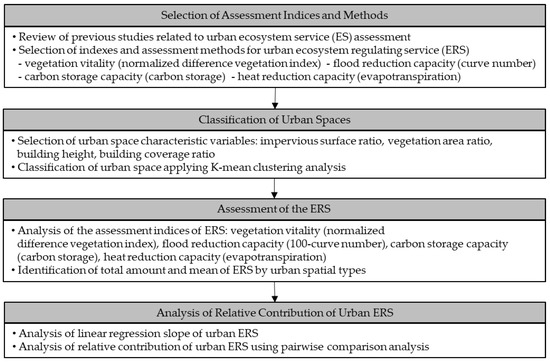
Figure 1.
Study procedure.
2.1. Selection of Assessment Indices and Methods
A regulating service is defined as the benefit of the regulatory function provided by the material cycle processes of an ecosystem [2,3,4]. In other words, it is possible to analyze a regulating service by calculating the enhancement in positive effects or reduction in negative environmental load so that the urban ecosystem can cycle virtuously. Additionally, the South Korean Ministry of Environment has recently focused on national research projects to improve vegetation vitality, flood reduction capacity, carbon storage capacity, and heat reduction capacity among ERS [41]. Moreover, policy efforts are being made to restore and promote the health of urban ecosystem by improving ERS through institutional means, such as urban environmental planning and environmental impact assessment. Therefore, this study selected vegetation vitality, flood reduction capacity, carbon storage capacity, and heat reduction capacity as the main assessment indices of urban ecosystem and based the assessment on the physical characteristic of the ERS.
Vegetation vitality refers to the distribution amount and vigor of vegetation, and the higher the vegetation vitality, the more active the growing state [21,42,43,44]. In addition, with higher vegetation vitality, better habitats can be created [21]. The regulating service increases the foundation for the virtuous cycle of the ecosystem [45,46]. In particular, numerous studies have shown that the higher the vegetation capacity, the greater the regulatory services, such as flood reduction capacity, carbon storage capacity, and heat reduction capacity [47,48]. Vegetation vitality can be assessed with a normalized difference vegetation index (NDVI) analysis, developed by Rouse et al. (1974) [42], using satellite images. In this study, the vegetation vitality of the study area was calculated by acquiring Landsat satellite images from days with low cloudiness and excellent vegetation vitality and analyzing the NDVI.
Furthermore, vegetation areas in the city contribute to flood prevention by storing rainwater, which delays the peak time and reduces the peak amount [22,23,49,50,51,52]. This effect can be estimated using the curve number (CN) value developed by the US Bureau of Land Management. CN is a coefficient used to estimate effective rainfall by analyzing detailed data on soil characteristics, cover condition, and preceding precipitation conditions [52,53]. CN is very useful in studies that calculate the flood reduction capacity of urban ecosystem that include green infrastructure. In this study, the South Korean runoff curve index according to land cover suggested by the South Korean Ministry of Environment was calculated considering the area occupied by each grid. The CN has a value between 0 and 100, and the closer the value is to 100, the higher the impermeability. For easy comparison with other regulating service assessment results, this study assessed the result of subtracting the CN value from 100 as the flood control ability.
Urbanization is accelerating climate change by causing increases in human activity and traffic, which emit greenhouse gases. Urban forests, parks, green spaces, and street trees absorb and store greenhouse gases in the atmosphere through photosynthesis [5,6,54,55]. This carbon storage capacity is calculated by dividing it into soil carbon storage and vegetation carbon storage. Soil carbon storage can be calculated using the carbon storage unit of each soil type, and vegetation carbon storage can be calculated using the biomass allometric equations according to IPCC guidelines (2006) [56].
Cities have the structural characteristic of discharging much heat because of land cover and buildings, and this discharge causes the urban heat island phenomenon [57,58,59,60]. Green infrastructure such as urban forests and street trees are attracting attention as important planning elements that can reduce such heat generation through transpiration [5,54,61,62,63]. This study assessed the heat reduction capacity of the area using evapotranspiration analysis by utilizing the EEFlux (Earth Engine Evapotranspiration Flux) model based on the Google Earth Engine system and Landsat 8 satellite image. Table 1 shows the definitions and analysis methods for the four aforementioned assessment indices.

Table 1.
Definition and analysis method of the ERS assessment indices.
2.2. Classification of Urban Spaces
Suwon City, the capital and largest city of Gyeonggi-do, South Korea with 1.2 million people occupying 12,100 hectares of land, was selected as the study area (Figure 2). Suwon City is basin-shaped and surrounded by mountains with various land uses, such as forests, agricultural land, and low-rise, mid-rise, and high-rise urbanization. Over the last decade, natural land cover such as forests and farmlands have decreased by about 9 km2 while urbanized areas have increased by about 6.3 km2. Despite such urbanization, further large-scale urban development projects are still being planned and carried out. In addition, with 40% of Suwon City comprising forests and farmlands, which provide a relatively large number of ES, it is an area where systematic urban ecosystem management is required.
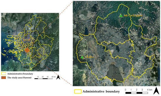
Figure 2.
The study area (Suwon City, Korea) (https://map.kakao.com/, accessed on 1 June 2021).
For spatial assessment of ERS, the study area was classified into a 60 m × 60 m grid by applying K-cluster analysis. The study area was classified into the 60 m × 60 m grid because satellite images, land cover maps, and soil maps produced by satellite images were mainly used as basic data for assessment of ES. There are 28,148 grids in the study area, and military facilities and areas under development were excluded from the analysis because of difficulties in obtaining data for analysis. In addition, water space was excluded because the selected indices are used mainly for measuring ERS of green areas.
2.3. Assessment of the ERS
The selected analysis methods were applied to assess the ERS of the study area. The ERS was analyzed by 60 m × 60 m grid resolution, and the level of urban ERS supply was identified using descriptive statistics analysis. In addition, by preparing the assessment results, regions with excellent and poor ERS supply were spatially identified. To compare ERS by urban spatial type, the total amount of services provided by each type and performance per grid (mean value) were analyzed. Thus, the types of space in which the ERS were excellently (or poorly) provided and the services that needed vast improvement were determined.
2.4. Analysis of Relative Contribution of Urban ERS
This study analyzed the relative contribution of each ERS by pairwise comparison in order to understand the interrelationship between them in detail. When there are multiple criteria in decision-making, pairwise comparison analysis is one of the leading methods used when estimating the significance (or importance) of several factors and details [67,68]. This method has an advantage to judge relative importance (contribution) of ERS in this study accurately [69]. A pair of two detailed elements is built to determine the relative importance, and such pairwise comparison is repeated to form a matrix of n assessment elements. The eigenvectors for each assessment element are calculated based on the constructed matrix, and the sum of the eigenvectors is 1. In other words, in a situation wherein the sum of all the elements of the ERS is assumed to be 1, the contribution of each element is determined based on the interrelationship. Based on this pairwise comparison analysis method, the relative contribution to the ERS was analyzed, as shown in Figure 3. The assessment results of the selected ERS need to be normalized because they have different units and scales. In this study, all the analysis results were normalized by 0–1 using the Min-Max method, as shown in Equation (1).
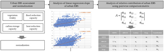
Figure 3.
Relative contribution analysis method between ERS.
Matrix A was then constructed by deriving slopes through linear regression slope analysis between ERS. In this study, a 4 × 4 matrix is formed because four regulating services have been selected. Next, the relative contribution was calculated by calculating the eigenvectors of the ERS elements based on the set matrix. In addition, the reliability of the analysis result was verified by checking the CI (Consistency Index) and CR (Consistency Ratio) values to diagnose the consistency of the calculated contribution.
The relative contribution of the ERS was calculated by dividing the entire study area by type of urban space, and the balance of the ERS was observed based on the analysis result. In other words, if the ERS selected in this study were ideally balanced, the eigenvector value would be equally calculated as 0.25. The balance of ERS by spatial type was diagnosed using the standard deviation of contribution.
3. Results
3.1. Results of Classification
Repeated K-cluster analysis confirmed that the number of samples (when the urban space of the study area was classified into six types) was distributed in a balanced manner. The study areas were forests (type A), agricultural land (type B), low-rise residential areas (type C), mid-rise mixed (residential and commercial) areas (type D), high-rise residential areas (type E), and industrial and barren land (type F) (Figure 4). The spatial characteristics of each type is shown in Table 2. The number of type A grids is 1.5 to 2.5 times larger than that of other types, with a total of 8378, and they are mainly forests on the periphery of the study area or parks and green spaces located sporadically inside the study area. Type B is located between type A and urbanized types C–F, and is mainly used for agricultural purposes. Among the six types, type C has the smallest vegetation area and the highest impermeability. In the case of type C, the building occupancy rate in the grid is 32.28%, which is very high compared to other types, and it is expected to provide the fewest ERS.
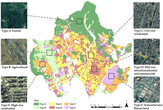
Figure 4.
Results of classification of the study area.
Table 2.
Spatial characteristics for six types of urban space.
3.2. Assessment Results of ERS
The NDVI within the study area has a range of −0.0032 to 0.88 with a mean of 0.45. The runoff curve index has a distribution of 8 to 33.67 with a mean of 20.38. The carbon storage capacity has a distribution of 2.48 to 60.42 tC/ha with a mean of 15.17 tC/ha, and in the case of evapotranspiration it is 0 to 1.09 with a mean of 0.21 (Table 3). For the entire study area, the difference between the maximum and minimum values is large for the regulating service assessment results, and the mean value is close to the minimum value. Hence, the large difference between maximum and minimum values indices means that there are various urban ecological spaces within the study area, and that the ERS are spatially imbalanced. In addition, the mean value is closer to the minimum value than the maximum value, and it can be inferred that the number of distributed artificial environments is larger than the number of natural ecological spaces. Such characteristics can also be confirmed from the map. While showing ample regulating services for the four indices in the north and west sides of the study area, where urban forests are mainly distributed, the regulating service for the central part of the study area, which has been heavily urbanized, is low. In addition, it has been confirmed that parks and green spaces located sporadically inside the city perform excellently for the ERS (Figure 5).
Table 3.
Descriptive statistics of ERS.
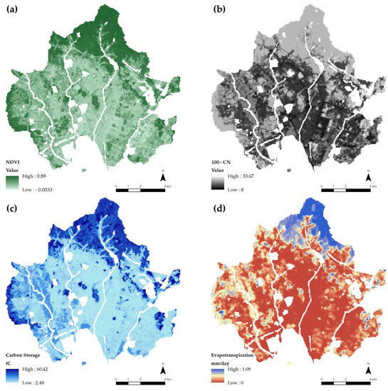
Figure 5.
ERS maps (a) vegetation vitality: NDVI; (b) flood reduction capacity: 100-CN; (c) carbon storage capacity: carbon storage capacity; (d) heat reduction capacity: evapotranspiration.
When the mean value of the regulating services for the six types, by type and grid (Table 4), are considered, type A is found to provide the most regulating services among all six types. Type A occupies 45% of the total area of the study area and provides 38% to 67% of total regulating services. Type B occupies 12.5% of the total area of the study area and provides 11% to 13% of the total ERS as well as the occupied area. Therefore, in order to prevent the deterioration of the ERS of the study area, it is necessary to restrain additional urban developments in type A and type B areas.
Table 4.
ERS for the entire study area and six types.
Meanwhile, type C (low-rise residential areas) shows low numbers for all regulating services. Type C also occupies 16% of the total study area while it provides only 2–12% of the total amount of regulating services. Hence, it is apparent that this type reduces the regulating services of the entire ecosystem of the study area. On the other hand, type D (mid-rise residential and commercial areas) and type E (high-rise residential) occupy an area similar to that of type C and they provide a slightly higher ERS than type C. However, the amount of ERS provided is still low (4% to 13%) compared with the amount of occupied area. Since type F covers a smaller area than the other types, a low mean value is distributed between types E and F. Therefore, it is necessary to expand green space in types C, D, and E in order to improve the regulating services of the urban ecosystem in the study area. With type C in particular, the building coverage ratio should be reduced, and afforestation should be actively encouraged for future urban planning and management.
3.3. Results of Relative Contribution Analysis
The results of linear regression slope analysis of each type are presented in Appendix A. The calculation results of the relative contributions obtained using the eigenvectors of the urban ERS for each type are the same as those shown in Table 5 and Figure 6. Both the CI and CR values, which are indices of the consistency of the eigenvectors, showed a significance level within 0.1, and the contribution analysis results were analyzed with the assumption that pairwise comparison was valid. The contribution of the ERS in the study area was in the order of heat reduction capacity (0.2964), flood reduction capacity (0.2815), carbon storage capacity (0.2374), and vegetation vitality (0.1847). It was confirmed that such contributions differ, depending on the type of urban space. Type A had the highest contribution in flood reduction, types B–E had the highest contribution in heat reduction, while type F had the highest contribution in carbon storage. In addition, all six types were similar in that they had the lowest contribution in vegetation vitality.
Table 5.
Results of pairwise comparison analysis of ERS (eigenvector values).
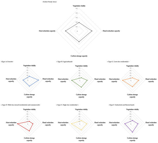
Figure 6.
Results of the relative contribution analysis of urban ERS spider diagram.
The standard deviations of the relative contributions by type show a distribution of 0.043 to 0.1460. The closer the standard deviation value is to 0, the better the regulating service is in ideal harmony. Considering the contribution of the entire study area, as the standard deviation is 0.0435, it is roughly balanced, but clearly the regulating service by type is not balanced. Type A has a standard deviation of 0.0744, which is the most harmonious regulating service compared with the other types, while types B–D have a standard deviation of 0.1 or greater. The reason for this is that the contribution of vegetation vitality within the region was calculated to be lower than that of other ERS.
4. Discussion
The main results of this study are as follows. Assessment of the ERS confirmed that type A forests were the best compared with other types in terms of total amount and mean value. On the other hand, type C low-rise residential ERS were underperforming in all metrics. In addition, the mean value in all assessment indices follows the same pattern: namely, the order of forest, agricultural land, industrial and barren land, high-rise residential area, residential and commercial mixed area, or low-rise residential area, except in the case of heat reduction capacity. Even within the same residential area, high-rise residential areas provide more ERS than low-rise residential areas. This is because a high-rise residential area has a higher building height than a low-rise residential area, but the proportion of the building area is low, and a green space is secured around the buildings. Such results suggest that damage to forests and agricultural land should be minimized to strengthen ERS in the city in the future, and roadside tree planting and rooftop greening should be actively encouraged when developing low-rise residential areas.
The relative contribution analysis between the ERS confirmed that although they are in harmony with each other in terms of the entire study area, imbalances are displayed when analyzing by type. In particular, the contribution of vegetation vitality was the lowest for all types, and such imbalances were higher in mid-rise mixed (residential and commercial) and low-rise residential areas than in other types. The NDVI shows the vitality of vegetation, and in order to achieve a balance of ERS in the study area, adequate growth conditions should be created to help vegetation thrive both quantitatively and qualitatively. Of course, ensuring vegetation growth in areas that are already heavily urbanized can be very difficult. However, as shown in a study by Kim, Oh, and Lee [70], there are many potential areas in the city that can be used for rooftop greening and roadside tree planting. Therefore, vegetation vitality can be increased above current levels if rooftop greening, and roadside are actively introduced and continuously managed to ensure healthy growth conditions.
This study has the following planning implications from the viewpoint of improving the regulating service of urban ecosystem. In the current climate change crisis, efforts to improve ES are increasing. Therefore, many local governments are making policy efforts to expand green park spaces in the city and secure more green spaces in planning urban development. Recently, there have been increasing efforts to secure urban ecological space in terms of quantity and increase the qualitative value of ecological spaces to harmonize with ES. In this study, we specifically confirmed the types and spatial characteristics of services that are excellently (or inadequately) supplied through the analysis of the interrelationships of urban ERS. Local governments that plan and manage urban ES can, based on the results of such analyses, establish alternatives that can maximize the effectiveness of their plans. For example, when ERS are preferentially supplied to spaces with low total amount and mean, such as low-rise residential, in order to improve the vegetation vitality with the lowest contribution, it is possible to strengthen and balance ERS simultaneously. Hence, the results of this study can provide a useful basis in determining priority areas and the supply needed in formulating urban green space plans and forest restoration plans.
5. Conclusions
This study focused on flood reduction capacity, carbon storage capacity, and heat reduction capacity in Suwon City, South Korea, and assessed the balance of ERS by type of urban eco-spaces. Analysis determined that six types of forest area ERS were the best in terms of total amount and mean value, with low-rise residential areas being the most vulnerable. In addition, although the results were relatively harmonious in diagnosing the balance between the researched ERS, most areas did not achieve the balance in relative contribution, except for the forest area.
Among the six urban spatial types, the standard deviation of the relative contribution of the mid-rise mixed (residential and commercial) area was the highest, at 0.14, confirming that the imbalance within the type was the most severe. This study spatially identified areas with insufficient supply of ERS and areas with an imbalance. Local governments that want to improve urban ES will be able to enhance project effectiveness using these research results if they want to prioritize the expansion of parks and green spaces and restoration projects in the lowest-grade type, which lack in total quantity and performance. In addition, in the case of types with a similar total amount it will be possible to contribute to the virtuous cycle of the urban ecosystem by checking the balance of detailed ERS for each type and intensively improving the factors that make up the imbalance. However, this study has the following limitations: in addition to the selected assessment indices, the urban ecosystem provides regulating services, such as air pollution reduction capacity. In order to diagnose the balance of ERS more accurately, a comprehensive analysis and interpretation of the regulatory services not considered in this study are required. In addition, the usefulness of this study could be further increased if type of forest (evergreen tree species or deciduous tree species), type of agricultural land (paddy, field, or orchard), rooftop greening, green walls, and water spaces are included in the next analysis. Nevertheless, this study diagnoses the balance of ERS based on the interrelationships of various ERS, and it will be useful in establishing spatial plans to improve of ERS.
Author Contributions
This article is the result of the joint work by all the authors. K.O. supervised and coordinated work on the paper. Conceptualization, K.O.; methodology, K.O.; validation, K.O. and D.L.; formal analysis, H.K.; data curation, H.K.; writing—original draft preparation, D.L.; writing—review and editing, K.O. and D.L.; visualization, H.K.; supervision, K.O.; project administration, K.O.; funding acquisition, K.O. All authors have read and agreed to the published version of the manuscript.
Funding
This research was funded by the Korea Ministry of Environment (MOE) grant number 2020002780001.
Institutional Review Board Statement
Not applicable.
Informed Consent Statement
Not applicable.
Data Availability Statement
Not applicable.
Acknowledgments
This work was conducted with the support of the Korea Environment Industry and Technology Institute (KEITI) through its Urban Ecological Health Promotion Technology Development Project.
Conflicts of Interest
The authors declare no conflict of interest.
Appendix A
Table A1.
Linear regression slopes: entire study area.
Table A1.
Linear regression slopes: entire study area.
| x-axis: NDVI–y-axis: 100-CN | x-axis: NDVI–y-axis: carbon storage |
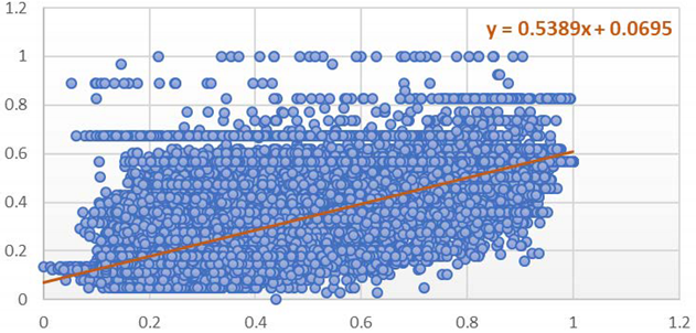 | 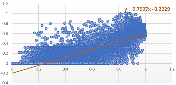 |
| Y = 0.5389x + 0.0695 | Y = 0.7997x − 0.2029 |
| x-axis: NDVI–y-axis: evapotranspiration | x-axis: 100-CN–y-axis: carbon storage |
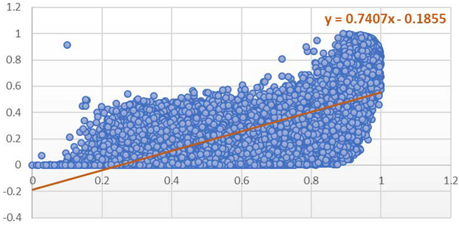 |  |
| Y = 0.7407x − 0.1855 | Y = 1.0384x − 0.1528 |
| x-axis: 100-CN–y-axis: evapotranspiration | x-axis: Carbon Storage–y-axis: evapotranspiration |
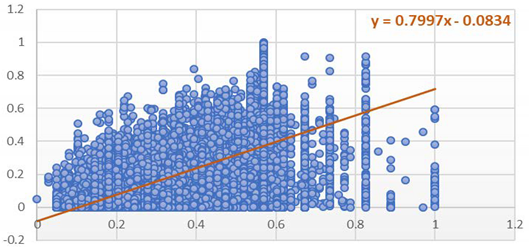 | 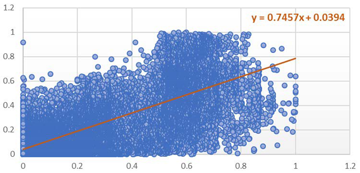 |
| Y = 0.7997x − 0.0834 | Y = 0.7457x + 0.0394 |
Table A2.
Linear regression slopes: type A.
Table A2.
Linear regression slopes: type A.
| x-axis: NDVI–y-axis: 100-CN | x-axis: NDVI–y-axis: carbon storage |
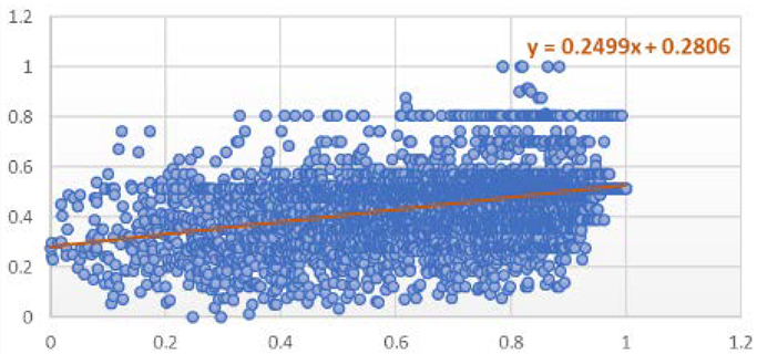 | 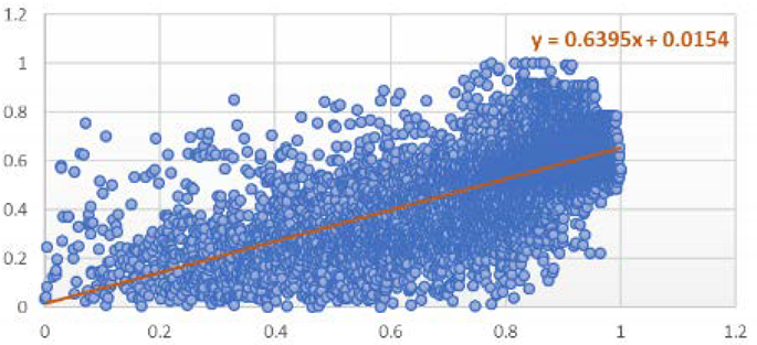 |
| Y = 0.2499x + 0.2806 | Y = 0.6395x + 0.0154 |
| x-axis: NDVI–y-axis: evapotranspiration | x-axis: 100-CN–y-axis: carbon storage |
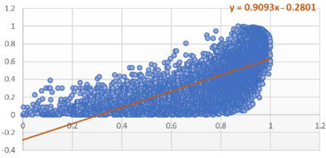 | 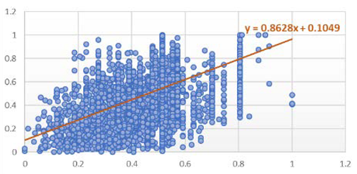 |
| Y = 0.9093x − 0.2801 | Y = 0.8628x + 0.1049 |
| x-axis: 100-CN–y-axis: evapotranspiration | x-axis: Carbon Storage–y-axis: evapotranspiration |
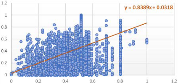 | 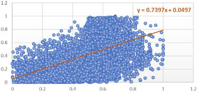 |
| Y = 0.8389x + 0.0318 | Y = 0.7397x + 0.0497 |
Table A3.
Linear regression slopes: type B.
Table A3.
Linear regression slopes: type B.
| x-axis: NDVI–y-axis: 100-CN | x-axis: NDVI–y-axis: carbon storage |
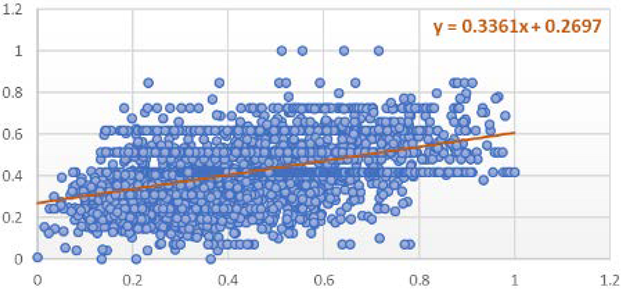 | 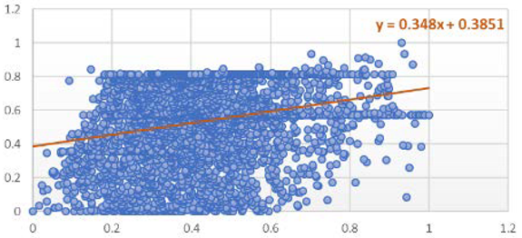 |
| Y = 0.3361x + 0.2697 | Y = 0.348x + 0.3851 |
| x-axis: NDVI–y-axis: evapotranspiration | x-axis: 100-CN–y-axis: carbon storage |
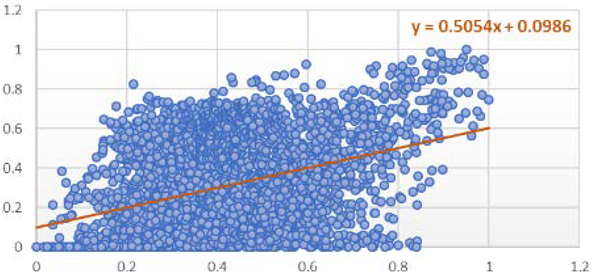 | 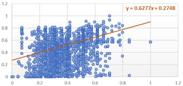 |
| Y = 0.5054x + 0.0986 | Y = 0.6277x + 0.2748 |
| x-axis: 100-CN–y-axis: evapotranspiration | x-axis: Carbon Storage–y-axis: evapotranspiration |
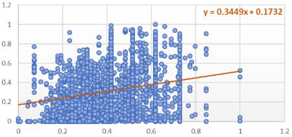 | 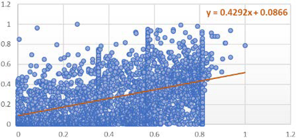 |
| Y = 0.3449x + 0.1732 | Y = 0.4292x + 0.0866 |
Table A4.
Linear regression slopes: type C.
Table A4.
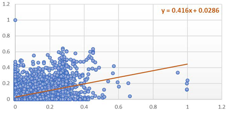
Linear regression slopes: type C.
| x-axis: NDVI–y-axis: 100-CN | x-axis: NDVI–y-axis: carbon storage |
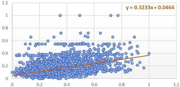 | 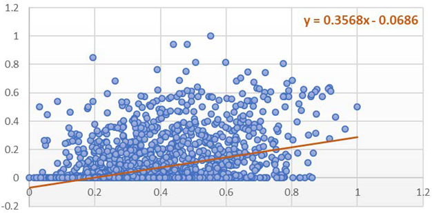 |
| Y = 0.3233x + 0.0464 | Y = 0.3568x − 0.0686 |
| x-axis: NDVI–y-axis: evapotranspiration | x-axis: 100-CN–y-axis: carbon storage |
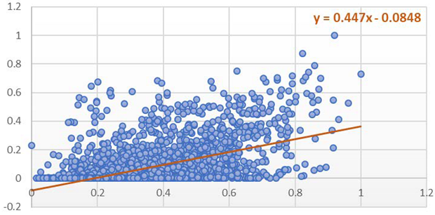 | 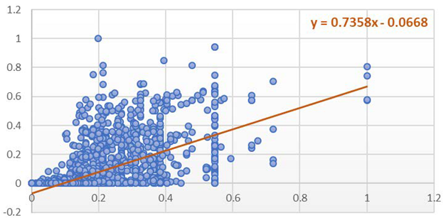 |
| Y = 0.447x − 0.0848 | Y = 0.7358x − 0.0668 |
| x-axis: 100-CN–y-axis: evapotranspiration | x-axis: Carbon Storage–y-axis: evapotranspiration |
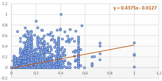 | 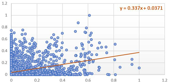 |
| Y = 0.4375x − 0.0127 | Y = 0.337x + 0.0371 |
Table A5.
Linear regression slopes: type D.
Table A5.
Linear regression slopes: type D.
| x-axis: NDVI–y-axis: 100-CN | x-axis: NDVI–y-axis: carbon storage |
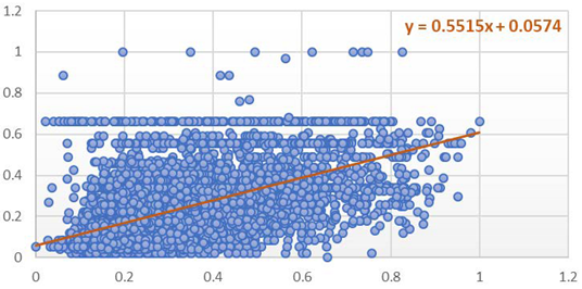 | 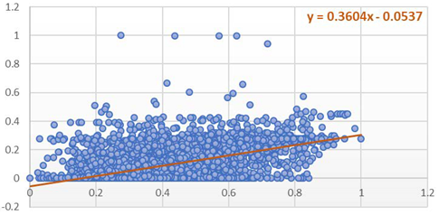 |
| Y = 0.5515x + 0.0574 | Y = 0.3604x − 0.0537 |
| x-axis: NDVI–y-axis: evapotranspiration | x-axis: 100-CN–y-axis: carbon storage |
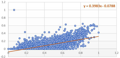 | 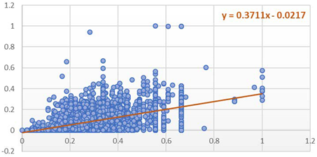 |
| Y = 0.3983x − 0.0788 | Y = 0.3711x − 0.0217 |
| x-axis: 100-CN–y-axis: evapotranspiration | x-axis: Carbon Storage–y-axis: evapotranspiration |
 |  |
| Y = 0.1901x − 0.0108 | Y = 0.416x + 0.0286 |
Table A6.
Linear regression slopes: type E.
Table A6.
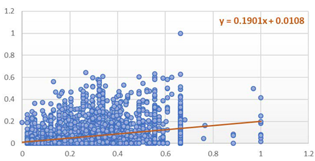
Linear regression slopes: type E.
| x-axis: NDVI–y-axis: 100-CN | x-axis: NDVI–y-axis: carbon storage |
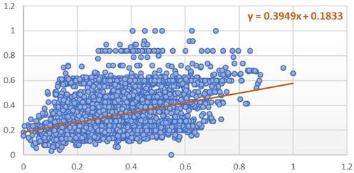 | 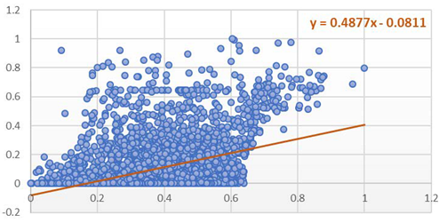 |
| Y = 0.3949x + 0.1833 | Y = 0.4877x − 0.0811 |
| x-axis: NDVI–y-axis: evapotranspiration | x-axis: 100-CN–y-axis: carbon storage |
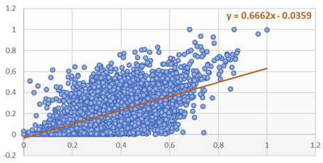 |  |
| Y = 0.6662x − 0.0359 | Y = 0.6462x − 0.1155 |
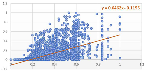
| x-axis: 100-CN–y-axis: evapotranspiration | x-axis: Carbon Storage–y-axis: evapotranspiration |
 | 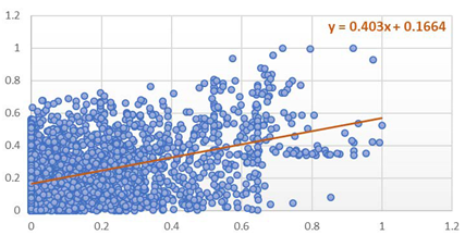 |
| Y = 0.3362x − 0.0951 | Y = 0.403x + 0.1664 |
Table A7.
Linear regression slopes: type F.
Table A7.
Linear regression slopes: type F.
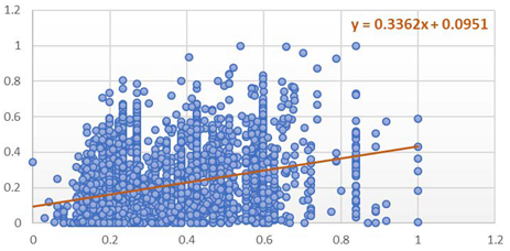
| x-axis: NDVI–y-axis: 100-CN | x-axis: NDVI–y-axis: carbon storage |
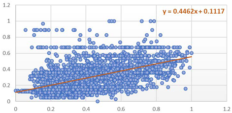 | 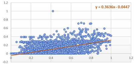 |
| Y = 0.4462x + 0.1117 | Y = 0.3636x − 0.0447 |
| x-axis: NDVI–y-axis: evapotranspiration | x-axis: 100-CN–y-axis: carbon storage |
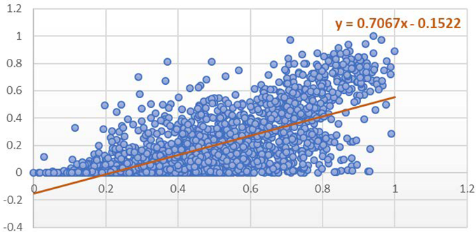 | 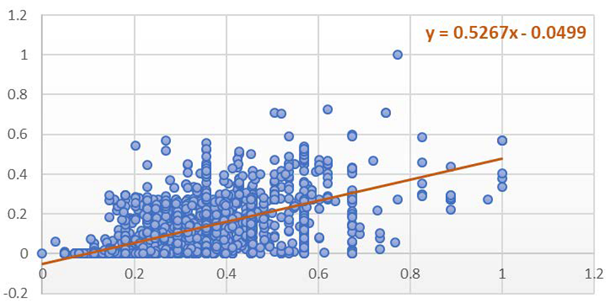 |
| Y = 0.7067x − 0.1522 | Y = 0.5267x − 0.0499 |
| x-axis: 100-CN–y-axis: evapotranspiration | x-axis: Carbon Storage–y-axis: evapotranspiration |
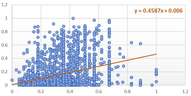 | 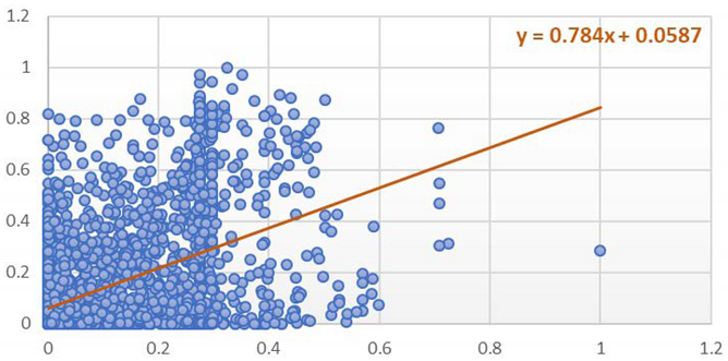 |
| Y = 0.4587x + 0.006 | Y = 0.784x + 0.0587 |
References
- Starfinger, U.; Sukopp, H. Assessment of Urban Biotopes for Nature Conservation; Elsevier: Amsterdam, The Netherlands, 1994; pp. 89–115. [Google Scholar]
- Corvalan, C.; Hales, S.; McMichael, A.; Butler, C.; Campbell-Lendrum, D.; Confalonieri, U.; Leitner, K.; Lewis, N.; Patz, J.; Polson, K.; et al. Ecosystems and Human Well-Being: Health Synthesis; WHO: Geneva, Switzerland, 2005. [Google Scholar]
- Costanza, R.; D’Arge, R.; De Groot, R.; Farber, S.; Grasso, M.; Hannon, B.; Limburg, K.; Naeem, S.; O’Neill, R.V.; Paruelo, J.M.; et al. The value of the world’s ecosystem services and natural capital. Nature 1997, 387, 253–260. [Google Scholar] [CrossRef]
- Daily, G.; Postel, S.; Bawa, K.; Kaufman, L. Nature’s Services: Societal Dependence on Natural Ecosystems; Bibliovault OAI Repository, the University of Chicago Press: Chicago, IL, USA, 1997. [Google Scholar]
- Cortinovis, C.; Geneletti, D. A framework to explore the effects of urban planning decisions on regulating ecosystem services in cities. Ecosyst. Serv. 2019, 38, 100946. [Google Scholar] [CrossRef]
- Holt, A.R.; Mears, M.; Maltby, L.; Warren, P. Understanding spatial patterns in the production of multiple urban ecosystem services. Ecosyst. Serv. 2015, 16, 33–46. [Google Scholar] [CrossRef] [Green Version]
- Derkzen, M.L.; van Teeffelen, A.; Verburg, P. REVIEW: Quantifying urban ecosystem services based on high-resolution data of urban green space: An assessment for Rotterdam, the Netherlands. J. Appl. Ecol. 2015, 52, 1020–1032. [Google Scholar] [CrossRef]
- Spake, R.; Lasseur, R.; Crouzat, E.; Bullock, J.M.; Lavorel, S.; Parks, K.E.; Schaafsma, M.; Bennett, E.M.; Maes, J.; Mulligan, M.; et al. Unpacking ecosystem service bundles: Towards predictive mapping of synergies and trade-offs between ecosystem services. Glob. Environ. Chang. 2017, 47, 37–50. [Google Scholar] [CrossRef] [Green Version]
- Zhang, Z.; Liu, Y.; Wang, Y.; Liu, Y.; Zhang, Y.; Zhang, Y. What factors affect the synergy and tradeoff between ecosystem services, and how, from a geospatial perspective? J. Clean. Prod. 2020, 257, 120454. [Google Scholar] [CrossRef]
- Gordon, A.; Simondson, D.; White, M.; Moilanen, A.; Bekessy, S.A. Integrating conservation planning and landuse planning in urban landscapes. Landsc. Urban Plan. 2009, 91, 183–194. [Google Scholar] [CrossRef]
- McShane, T.O.; Hirsch, P.D.; Trung, T.C.; Songorwa, A.; Kinzig, A.; Monteferri, B.; Mutekanga, D.; Van Thang, H.; Dammert, J.L.; Pulgar-Vidal, M.; et al. Hard choices: Making trade-offs between biodiversity conservation and human well-being. Biol. Conserv. 2011, 144, 966–972. [Google Scholar] [CrossRef]
- Rodríguez, J.P.; Beard, J.T.D.; Bennett, E.M.; Cumming, G.; Cork, S.J.; Agard, J.; Dobson, A.P.; Peterson, G. Trade-offs across Space, Time, and Ecosystem Services. Ecol. Soc. 2006, 11. [Google Scholar] [CrossRef] [Green Version]
- Haase, D.; Schwarz, N.; Strohbach, M.; Kroll, F.; Seppelt, R. Synergies, Trade-offs, and Losses of Ecosystem Services in Urban Regions: An Integrated Multiscale Framework Applied to the Leipzig-Halle Region, Germany. Ecol. Soc. 2012, 17, 22. [Google Scholar] [CrossRef]
- Jia, X.; Fu, B.; Feng, X.; Hou, G.; Liu, Y.; Wang, X. The tradeoff and synergy between ecosystem services in the Grain-for-Green areas in Northern Shaanxi, China. Ecol. Indic. 2014, 43, 103–113. [Google Scholar] [CrossRef]
- Qin, K.; Lin, Y.-P.; Yang, X. Trade-Off and Synergy among Ecosystem Services in the Guanzhong-Tianshui Economic Region of China. Int. J. Environ. Res. Public Health 2015, 12, 14094–14113. [Google Scholar] [CrossRef]
- Turkelboom, F.; Thoonen, M.; Jacobs, S.; Garcia Llorente, M.; Martín-López, B.; Berry, P. Ecosystem Services Trade-Offs and Synergies; OpenNESS: Helsinki, Finland, 2016. [Google Scholar] [CrossRef]
- Hao, R.; Yu, D.; Wu, J. Relationship between paired ecosystem services in the grassland and agro-pastoral transitional zone of China using the constraint line method. Agric. Ecosyst. Environ. 2017, 240, 171–181. [Google Scholar] [CrossRef]
- Lin, S.; Wu, R.; Yang, F.; Wang, J.; Wu, W. Spatial trade-offs and synergies among ecosystem services within a global biodiversity hotspot. Ecol. Indic. 2018, 84, 371–381. [Google Scholar] [CrossRef]
- Tallis, H.; Kareiva, P.; Marvier, M.; Chang, A. An ecosystem services framework to support both practical conservation and economic development. Proc. Natl. Acad. Sci. USA 2008, 105, 9457–9464. [Google Scholar] [CrossRef] [PubMed] [Green Version]
- Oh, K.; Lee, D.; Park, C. Urban Ecological Network Planning for Sustainable Landscape Management. J. Urban Technol. 2011, 18, 39–59. [Google Scholar] [CrossRef]
- Lee, D.; Oh, K. The Green Infrastructure Assessment System (GIAS) and Its Applications for Urban Development and Management. Sustainability 2019, 11, 3798. [Google Scholar] [CrossRef] [Green Version]
- Armson, D.; Stringer, P.; Ennos, A. The effect of street trees and amenity grass on urban surface water runoff in Manchester, UK. Urban For. Urban Green. 2013, 12, 282–286. [Google Scholar] [CrossRef]
- Zhang, B.; Xie, G.-D.; Li, N.; Wang, S. Effect of urban green space changes on the role of rainwater runoff reduction in Beijing, China. Landsc. Urban Plan. 2015, 140, 8–16. [Google Scholar] [CrossRef]
- Frank, B.; Delano, D.; Caniglia, B.S. Urban systems: A socio-ecological system perspective. Sociol. Int. J. 2017, 1, 1–8. [Google Scholar] [CrossRef] [Green Version]
- Grimm, N.B.; Redman, C.L.; Boone, C.G.; Childers, D.L.; Harlan, S.L.; Turner, B.L. Viewing the urban socio-ecological system through a sustainability lens: Lessons and prospects from the central Arizona–Phoenix LTER programme. In Long Term Socio-Ecological Research; Springer: Berlin/Heidelberg, Germany, 2013; pp. 217–246. [Google Scholar] [CrossRef]
- Felipe-Lucia, M.R.; Comín, F.A.; Escalera-Reyes, J. A framework for the social valuation of ecosystem services. AMBIO 2014, 44, 308–318. [Google Scholar] [CrossRef] [Green Version]
- Raudsepp-Hearne, C.; Peterson, G.; Bennett, E.M. Ecosystem service bundles for analyzing tradeoffs in diverse landscapes. Proc. Natl. Acad. Sci. USA 2010, 107, 5242–5247. [Google Scholar] [CrossRef] [Green Version]
- Davies, Z.G.; Edmondson, J.L.; Heinemeyer, A.; Leake, J.R.; Gaston, K.J. Mapping an urban ecosystem service: Quantifying above-ground carbon storage at a city-wide scale. J. Appl. Ecol. 2011, 48, 1125–1134. [Google Scholar] [CrossRef] [Green Version]
- White, C.; Halpern, B.S.; Kappel, C.V. Ecosystem service tradeoff analysis reveals the value of marine spatial planning for multiple ocean uses. Proc. Natl. Acad. Sci. USA 2012, 109, 4696–4701. [Google Scholar] [CrossRef] [Green Version]
- Gómez-Baggethun, E.; Barton, D.N. Classifying and valuing ecosystem services for urban planning. Ecol. Econ. 2012, 86, 235–245. [Google Scholar] [CrossRef]
- Chan, K.M.A.; Satterfield, T. Managing Cultural Ecosystem Services for Sustainability; Routledge: London, UK, 2016; pp. 343–358. [Google Scholar] [CrossRef] [Green Version]
- Korea Ministry of Environment (KME). Basic Plan for Conservation of the Natural Environment; Korea Ministry of Environment (KME): Sejong, Korea, 2015. [Google Scholar]
- TEEB. The Economics of Ecosystem and Biodiversity, Mainstreaming the Economics of Nature: A Synthesis of the Approach, Conclusions and Recommendations of TEEB; UNEP: Ginebra, Switzerland, 2012. [Google Scholar]
- Song, I.; Yoon, C. Establishment and Utilization of Ecosystem Service Assessment in Seoul; Seoul Institute: Seoul, Korea, 2019; Volume 2019. [Google Scholar]
- Crookes, D.; Blignaut, J.; de Wit, M.; Esler, K.; Le Maitre, D.; Milton, S.; Mitchell, S.; Cloete, J.; de Abreu, P.; Vlok, H.F.; et al. System dynamic modelling to assess economic viability and risk trade-offs for ecological restoration in South Africa. J. Environ. Manag. 2013, 120, 138–147. [Google Scholar] [CrossRef] [PubMed] [Green Version]
- Lauf, S.; Haase, D.; Kleinschmit, B. Linkages between ecosystem services provisioning, urban growth and shrinkage—A modeling approach assessing ecosystem service trade-offs. Ecol. Indic. 2014, 42, 73–94. [Google Scholar] [CrossRef]
- Balbi, S.; del Prado, A.; Gallejones, P.; Geevan, C.P.; Pardo, G.; Pérez-Miñana, E.; Manrique, R.; Hernandez-Santiago, C.; Villa, F. Modeling trade-offs among ecosystem services in agricultural production systems. Environ. Model. Softw. 2015, 72, 314–326. [Google Scholar] [CrossRef] [Green Version]
- Lee, H.; Lautenbach, S. A quantitative review of relationships between ecosystem services. Ecol. Indic. 2016, 66, 340–351. [Google Scholar] [CrossRef]
- Burkhard, B.; Kroll, F.; Nedkov, S.; Müller, F. Mapping ecosystem service supply, demand and budgets. Ecol. Indic. 2012, 21, 17–29. [Google Scholar] [CrossRef]
- Chen, W.; Chi, G.; Li, J. The spatial aspect of ecosystem services balance and its determinants. Land Use Policy 2019, 90, 104263. [Google Scholar] [CrossRef]
- Korea Ministry of Environment (KME). Urban Ecological Health Promotion Technology Development Project; Korea Ministry of Environment (KME): Sejong, Korea, 2018. [Google Scholar]
- Rouse, J.W.; Haas, R.H.; Schell, J.A.; Deering, D.W. Monitoring vegetation systems in the great plains with ERTS. In Proceedings of the 3rd ERTS-1 Symposium, Washington, DC, USA, 10–14 December 1974; pp. 309–317. [Google Scholar]
- Weier, J.; Herring, D. Measuring Vegetation (NDVI & EVI). 2014. Available online: http://earthobservatory.nasa.gov/Features/MeasuringVegetation (accessed on 1 June 2021).
- Rozario, P.; Oduor, P.; Kotchman, L.; Kangas, M. Transition Modeling of Land-Use Dynamics in the Pipestem Creek, North Dakota, USA. J. Geosci. Environ. Prot. 2017, 5, 182–201. [Google Scholar] [CrossRef]
- Pettorelli, N.; Vik, J.O.; Mysterud, A.; Gaillard, J.-M.; Tucker, C.J.; Stenseth, N.C. Using the satellite-derived NDVI to assess ecological responses to environmental change. Trends Ecol. Evol. 2005, 20, 503–510. [Google Scholar] [CrossRef]
- Muratet, A.; Lorrillière, R.; Clergeau, P.; Fontaine, C. Evaluation of landscape connectivity at community level using satellite-derived NDVI. Landsc. Ecol. 2012, 28, 95–105. [Google Scholar] [CrossRef]
- De Carvalho, R.M.; Szlafsztein, C.F. Urban vegetation loss and ecosystem services: The influence on climate regulation and noise and air pollution. Environ. Pollut. 2018, 245, 844–852. [Google Scholar] [CrossRef] [PubMed]
- Mirsanjari, M.M.; Zarandian, A.; Mohammadyari, F.; Visockiene, J.S. Investigation of the impacts of urban vegetation loss on the ecosystem service of air pollution mitigation in Karaj metropolis, Iran. Environ. Monit. Assess. 2020, 192, 1–23. [Google Scholar] [CrossRef] [PubMed]
- Weng, Q. Modeling Urban Growth Effects on Surface Runoff with the Integration of Remote Sensing and GIS. Environ. Manag. 2001, 28, 737–748. [Google Scholar] [CrossRef]
- Nedkov, S.; Boyanova, K.; Burkhard, K. Quantifying, Modelling and Mapping Ecosystem Services in Watersheds; Springer: Dordrecht, The Netherlands, 2015; pp. 133–149. [Google Scholar] [CrossRef]
- Liu, W.; Chen, W.; Peng, C. Influences of setting sizes and combination of green infrastructures on community’s stormwater runoff reduction. Ecol. Model. 2015, 318, 236–244. [Google Scholar] [CrossRef]
- Mockus, V. National Engineering Handbook; US Soil Conservation Service: Washington, DC, USA, 1964; p. 4. [Google Scholar]
- Korea Ministry of Environment (KME). Standard Guidelines for Estimating Flood Volumes; Korea Ministry of Environment (KME): Sejong, Korea, 2019. [Google Scholar]
- Whitford, V.; Ennos, A.R.; Handley, J.F. “City form and natural process” indicators for the ecological performance of urban areas and their application to Merseyside, UK. Landsc. Urban Plan. 2001, 57, 91–103. [Google Scholar] [CrossRef]
- Nowak, D.J.; Crane, D.E. Carbon storage and sequestration by urban trees in the USA. Environ. Pollut. 2001, 116, 381–389. [Google Scholar] [CrossRef]
- Eggleston, H.S.; Buendia, L.; Miwa, K.; Ngara, T.; Tanabe, K. 2006 IPCC Guidelines for National Greenhouse Gas Inventories; IPCC National Greenhouse Gas Inventories Programme: Hayama, Japan, 2006. [Google Scholar]
- Grimmond, S. Urbanization and global environmental change: Local effects of urban warming. Geogr. J. 2007, 173, 83–88. [Google Scholar] [CrossRef]
- Stewart, I.D.; Oke, T.R. Local Climate Zones for Urban Temperature Studies. Bull. Am. Meteorol. Soc. 2012, 93, 1879–1900. [Google Scholar] [CrossRef]
- Lee, D.; Oh, K. Classifying urban climate zones (UCZs) based on statistical analyses. Urban Clim. 2018, 24, 503–516. [Google Scholar] [CrossRef]
- Lee, D.; Oh, K.; Jung, S. Classifying Urban Climate Zones (UCZs) Based on Spatial Statistical Analyses. Sustainability 2019, 11, 1915. [Google Scholar] [CrossRef] [Green Version]
- Larondelle, N.; Lauf, S. Balancing demand and supply of multiple urban ecosystem services on different spatial scales. Ecosyst. Serv. 2016, 22, 18–31. [Google Scholar] [CrossRef]
- Park, J.; Kim, J.-H.; Lee, D.K.; Park, C.Y.; Jeong, S.G. The influence of small green space type and structure at the street level on urban heat island mitigation. Urban For. Urban Green. 2017, 21, 203–212. [Google Scholar] [CrossRef]
- Lee, D.; Oh, K. Developing the Urban Thermal Environment Management and Planning (UTEMP) System to Support Urban Planning and Design. Sustainability 2019, 11, 2224. [Google Scholar] [CrossRef] [Green Version]
- Park, E.; Kang, K. Estimation of C Storage and Annual CO2 Uptake by Street Trees in Gyeonggi-do. Korean J. Environ. Ecol. 2010, 24, 591–600. [Google Scholar]
- Korea Forest Service. Carbon Emission Factors and Biomass Allometric Equations by Species in Korea; Korea Forest Service: Daejeon, Korea, 2006. [Google Scholar]
- Irmak, A. Evapotranspiration—Remote Sensing and Modeling; INTECH Open Access Publisher: London, UK, 2011. [Google Scholar]
- Saaty, T.L. Decision-making with the AHP: Why is the principal eigenvector necessary. Eur. J. Oper. Res. 2003, 145, 85–91. [Google Scholar] [CrossRef]
- Saaty, T.L. Decision making for leaders. IEEE Trans. Syst. Man Cybern. 1985, SMC-15, 450–452. [Google Scholar] [CrossRef]
- Oh, K.; Jeong, Y. The Usefulness of the GIS—Fuzzy Set Approach in Evaluating the Urban Residential Environment. Environ. Plan. B Plan. Des. 2002, 29, 589–606. [Google Scholar] [CrossRef] [Green Version]
- Kim, H.; Oh, K.; Lee, D. Establishment of a Geographic Information System-Based Algorithm to Analyze Suitable Locations for Green Roofs and Roadside Trees. Appl. Sci. 2021, 11, 7368. [Google Scholar] [CrossRef]
Publisher’s Note: MDPI stays neutral with regard to jurisdictional claims in published maps and institutional affiliations. |
© 2021 by the authors. Licensee MDPI, Basel, Switzerland. This article is an open access article distributed under the terms and conditions of the Creative Commons Attribution (CC BY) license (https://creativecommons.org/licenses/by/4.0/).