A Scalable Moving Boundary Treatment in the Lattice Boltzmann Method

Abstract

Based on the lattice Boltzmann Method (LBM), a new moving boundary treatment is proposed by studying the influence of the moving boundary in a low-speed incompressible fluid. Simulating flow past a static cylinder, flow past a moving cylinder, and flow in a curved moving pipe shows that the LBM has high reliability and stability with moving boundary conditions. In order to reduce parallel computing time and take full advantage of the characteristics of the model, the solid grids are allocated according to the number of computing cores. Two parallel speedup ratios were tested, keeping the overall task volume unchanged to increase the number of cores and keeping the single-core task volume unchanged. In the first speedup ratio, the efficiency of the flow field calculation at 112 cores reached more than 80%. The second speedup ratio indicated that the proportion of communication in the program was tiny and suitable for large-scale parallel computing. The study of the moving boundary problem can effectively help solve the fluid-structure coupling problem. Due to the particularity of the model, it can be used to simulate the fluid-structure coupling problem of blood vessel flow effectively.

1. Introduction

The problem of complex fluid flow has always been one of the most critical and challenging research fields in large-scale scientific and engineering computing. From a mesoscopic perspective, the lattice Boltzmann method (LBM), which originated from the lattice Gas Cellular Automata (LGA) method, is characterized by its simplicity and efficiency [1]. Due to the kinematic characteristics of the Boltzmann equation itself, the pressure field and local stress tensor can be directly obtained without solving the pressure Poisson problem. The feature makes LBM significantly suitable for large-scale parallel computing of complex flow problems [2]. This method has been widely used in many fields, such as two-dimensional multiphase flow [3], microscale fluid flow, biomechanics [4], and porous media [5]. However, there are problems in actual flow calculations, such as large computational grids, slow convergence speed, and weak numerical stability [6,7]. In calculating the single relaxation time lattice Boltzmann model (SRT-LBM), this shortcoming can be overcome with the help of some turbulence model methods. Based on the eddy viscosity model theory, Hou et al. [8] introduced the Smagorinsky vortex viscosity model into SRT-LBM, which effectively improved the Reynolds number limit of SRT-LBM and improved the flexibility of the algorithm. Hence, the followup research direction of this article is vascular fluid–solid coupling. The computational fluid is two-dimensional blood in the current research, and the Reynolds number is relatively low. SRT-LBM is sufficient to meet the needs of simulation.

One of the most concerning issues in computational fluid dynamics is the fluid-structure coupling problem. One of the main challenges in solving the fluid-structure coupling problem is the moving boundary problem. Ladd [9] first proposed a Bounce Back (BB) method to deal with motion boundary problems in 1993. Based on this curve boundary processing method, many researchers [10,11,12,13,14,15,16] have expanded and improved to reduce the frequency fluctuation caused by the movement of grid points. In 2018, Wei et al. [17] used the improved BB method to calculate the solid near and far areas by setting the main grid and the subgrid and proposed a floating grid method to deal with moving boundary problems. Because the immersion boundary method (IBM) is based on the Cartesian coordinate system and is suitable for combination with LBM, the application of IBM [18,19,20,21,22,23,24] in LBM is also another widely used moving boundary processing method.

2. D2G9 Model

A complete lattice Boltzmann model usually consists of the discrete velocity model, equilibrium distribution function, and distribution function evolution equation. In 1992, for the two-dimensional model, Qian et al. proposed the D2Q9 model [25] as the basic model of LBM. Many scholars have developed different models to solve problems in various application environments. The macroequation derived from the basic D2Q9 model is the compressible Navier-Stokes equation, so there will be an inevitable compression error when simulating incompressible flow. Since the followup research in this paper is the fluid–solid coupling problem of blood vessels, the computational fluid is blood under the assumption of incompressibility. For incompressible flow, people have developed a variety of incompressible lattice Boltzmann models [26,27,28]. Guo [29] proposed an incompressible model of D2G9, which has the characteristic that the sum of the balanced distribution functions is equal to a constant.

In the Cartesian coordinate system, the D2G9 model is the same as the discrete velocity model of the D2Q9 model. It can be seen from Equation (1) that the evolution equation of this incompressible model is the same as that of the classic D2Q9 model, which transforms the complex collision migration process into a relaxation process.

$$f_i\left(x+e_i,t+1\right)=\left(1-\tau \right)f_i\left(x,t\right)+\omega f_i^{eq}\left(x,t\right)$$

(1)

$f_i\left(x,t\right)$ is the probability density distribution function at the grid point x at time t after being discretized by the discrete velocity model. $f_i^{eq}\left(x,t\right)$ is the local equilibrium distribution function under the current macroscopic quantity, and the relaxation factor τ is related to the viscosity coefficient $\nu$. In SRT-LBM, the expression is $\tau =\nu c_s^2/\Delta t+0.5$ in which $c_s$ is the speed of sound and $\Delta t$ is the time step. Different from the D2Q9 model, the D2G9 model selects a new equilibrium distribution function, and the new equilibrium distribution function $g_i^{\left(0\right)}$ is given by the equation group (2):

$$g_i^{\left(0\right)}=\left\{\begin{array}{c}-4\sigma \frac{p}{c^2}+s_0\left(\mathit{u}\right) i=0\\ \lambda \frac{p}{c^2}+s_i\left(\mathit{u}\right) i=1,2,3,4\\ \gamma \frac{p}{c^2}+s_i\left(\mathit{u}\right) i=5,6,7,8\end{array}\right.$$

(2)

In the equation group (2)

$$s_i\left(\mathit{u}\right)={\omega }_i\left[3\frac{\left({\mathit{e}}_i\cdot \mathit{u}\right)}{c}+4.5\frac{{\left({\mathit{e}}_i\cdot \mathit{u}\right)}^2}{c^2}-1.5\frac{{\left|\mathit{u}\right|}^2}{c^2}\right]$$

(3)

The calculation formula of the macroscopic quantity is

$$\mathit{u}={\displaystyle \sum }_{i=1}^{8}c{\mathit{e}}_i{g}_i,p=\frac{c^2}{4\sigma }\left[{\displaystyle \sum }_{i=1}^8{g}_i+s_0\left(\mathit{u}\right)\right]$$

(4)

where u is the velocity vector and p is the pressure. $c=\Delta x/\Delta t$, $\Delta x$ is the grid interval. ${\omega }_i$ is the weight coefficient, which is the same as the weight coefficient of D2Q9. ${\mathit{e}}_i$ is the discrete speed, which is the same as the speed configuration of D2Q9. $g_i$ is the distribution function, which is obtained after collision migration. $\sigma$, and $\gamma$ are model parameters, which satisfy the following equations:

$$\left\{\begin{array}{c}\mathit{\lambda }+\mathit{\gamma }=\mathit{\sigma }\\ \mathit{\lambda }+\mathbf{2}\mathit{\gamma }=\mathbf{1}/\mathbf{2}\end{array}\right.$$

(5)

The reference values that can be selected are $\lambda =1/3,\gamma =1/12$.

In the D2G9 model, pressure replaces the density as an independent variable, and the standard incompressible Navier-Stokes equations can be derived, effectively eliminating the compressibility error of the D2Q9 model. In the calculation Formula (4) of macroscopic pressure, it can also be seen that the calculation of pressure is unrelated to density.

3. The Proposed Solid Boundary Condition

One of the advantages of solving flow problems through the Boltzmann equation is that it can easily solve complex solid boundary problems. For stationary boundary problems, the nonequilibrium state extrapolation format is used for processing when the boundary is straight; the unified boundary processing method proposed by Dazhi et al. [15] in 2003 is used when the boundary is curved. The method considers the problem of moving boundaries and can be directly applied to boundary processing when the grid point type does not change. When the grid point type changes, this method does not work and needs to be modified.

As shown in Figure 1a, a straight boundary is used instead of a curved boundary for ease of presentation. It should be noted that to clearly describe the problem of boundary movement, resulting in the loss of the new fluid point distribution function, the solid line here is designed as a straight line. The solid line can be any irregular curve approximated by an irregular polyline connected by a series of points. In Figure 1a, the solid black line is formed by connecting the red solid points, and the intersection of the broken line and the grid line is a hollow five-corner point. The relative distance between the intersection and the grid node can approximate the influence of the actual boundary. The relative distance $\Delta =\left|{\mathit{x}}_f-{\mathit{x}}_w\right|/\left|{\mathit{x}}_f-{\mathit{x}}_b\right|$. The grid point types of different grid points according to the position of the boundary are judged. Various signs are given in Figure 1a. Figure 1b shows the eight discrete velocity directions in the D2G9 model.

Taking the point ${\mathit{x}}_f$ in Figure 1a as an example, the distribution function of direction $\overline{\alpha }=3$ cannot be obtained by migration in the unified boundary processing format [15], which is given by Formula (6) below.

$${\mathit{f}}_{\overline{\alpha }}\left({\mathit{x}}_{\mathit{f}}\right)=\frac{\mathbf{1}}{\mathbf{1}+\mathbf{\Delta }}\left[\Delta {\mathit{f}}_{\overline{\mathit{\alpha }}}\left({\mathit{x}}_{\mathit{f}}\right)+\Delta {\mathit{f}}_{\mathit{\alpha }}\left({\mathit{x}}_{\mathit{f}}\right)+\left(\mathbf{1}-\Delta \right){\mathit{f}}_{\mathit{\alpha }}\left({\mathit{x}}_{\mathit{f}\mathit{f}}\right)+\mathbf{2}{\mathit{\omega }}_{\mathit{\alpha }}{\mathit{\rho }}_{\mathit{w}}\frac{\mathbf{3}}{{\mathit{c}}^{\mathbf{2}}}{\mathit{e}}_{\mathit{\alpha }}{\mathit{u}}_{\mathit{w}}\right]$$

(6)

where ${\mathit{e}}_{\mathit{\alpha }}$ is the discrete velocity and ${\mathit{\omega }}_{\mathit{\alpha }}$ is the weight coefficient. The right side of the equation is the distribution function before migration after a collision.

The unknown distribution function of the fluid boundary point can be solved directly by Formula (6) when the grid point type has not changed. When the type changes, for example, the boundary in Figure 1a moves from position 1-1 to position 4-4. For the point ${\mathit{x}}_b$, since $f_{\overline{\alpha }}\left({\mathit{x}}_b\right)$ in Formula (6) has not been calculated before the boundary movement, the specific value is not given. A simple processing method is to perform a second-order extrapolation of the solid boundary point distribution function along a specific discrete velocity direction before the type is changed [30]. The distribution function of the point ${\mathit{x}}_b$ is constructed by Formula (7).

$${\mathit{f}}_{\overline{\alpha }}\left({\mathit{x}}_{\mathit{b}}\right)=\mathbf{3}{\mathit{f}}_{\overline{\alpha }}\left({\mathit{x}}_{\mathit{f}}\right)-\mathbf{3}{\mathit{f}}_{\overline{\alpha }}\left({\mathit{x}}_{\mathit{f}\mathit{f}}\right)+{\mathit{f}}_{\overline{\alpha }}\left({\mathit{x}}_{\mathit{f}\mathit{f}}+{\mathit{e}}_{\mathbf{3}}\right)$$

(7)

This method maintains the continuity of the fluid before and after the exercise. Based on Formula (7) and considering the efficiency in parallel computing, the data transfer process between adjacent processes should be as simplified as possible. Before the grid point type changes, the solid point velocity is interpolated by the fluid boundary point velocity in a specific direction. The pressure is the pressure corresponding to the fluid boundary point. The equilibrium distribution function calculated by the macroscopic quantity of this point is used as the initial value of the new fluid boundary point, as shown in Formula (8).

$$\left\{\begin{array}{c}{\mathit{u}}_{\mathit{b}}=\left[\left.{\mathit{u}}_{\mathit{w}}+\left(\Delta -\mathbf{1}\right){\mathit{u}}_{\mathit{f}}\right]/\Delta \right.\\ {\mathit{p}}_{\mathit{b}}={\mathit{p}}_{\mathit{f}}\\ \mathit{f}\left({\mathit{x}}_{\mathit{b}}\right)={\mathit{f}}^{\mathit{e}\mathit{q}}\left({\mathit{p}}_{\mathit{b}},{\mathit{u}}_{\mathit{b}}\right)\end{array}\right.$$

(8)

The specific direction is the discrete velocity direction corresponding to when $\mathit{n}\cdot {\mathit{e}}_{\mathit{\alpha }}$ is maximized.

In order to show the effect of this correction, there is a two-dimensional cylinder moving horizontally and at a constant speed in the rectangular calculation domain with an open boundary to observe the pressure field distribution around the cylinder in the early development stage. Due to the horizontal movement to the right, only the solid grid points at the left end of the cylinder become fluid grid points. In the early stage, there is only a pressure gradient around the cylinder. Observe the local pressure field distribution around the cylinder, as shown in Figure 2. It can be seen from Figure 2a that compared with the left end of the cylinder, the pressure graph at the left end of the cylinder has a jagged feeling. After correction, compared with Figure 2a, the jaggedness of the flow field in the red box in Figure 2b is significantly reduced, indicating that this correction can alleviate the problem of the missing distribution function of the new fluid grid points. This article only adds a new fluid point initialization method based on the original boundary format. The overall method is relatively concise, it is easy to program, and it can also meet the needs of moving boundary problem simulation. Since this article directly expands the existing format, the accuracy is only affected by the grid size.

4. Mesh Generation for a Specific Model

In Figure 3, a flow chart of the static boundary and the moving boundary of the LBM is presented simultaneously. For the stationary boundary problem, the calculation process is shown by the black arrow. For the moving boundary problem, in the judgment of the sixth step, turn to the process shown by the red arrow, and add the eighth and ninth steps. In the ninth step, use Formula (8) proposed to initialize the new fluid point. It should be noted that the new cycle starts before the second step in the moving boundary problem. This means that each cycle includes a grid generation process, which will increase the time overhead. Therefore, optimized mesh generation can significantly reduce the total calculation time for the parallel calculation of moving boundary problems.

In mesh generation, three kinds of information about the grid need to be obtained: one, the grid style: solid grid or fluid grid; two, the boundary style: grid is or is not near the solid boundary; three, the distance: the distance from the boundary grid point to the solid boundary. In serial calculations, the three types of grid information can be easily obtained through the internal point connection method. The line segment formed by the point to be judged and the known internal point has a certain number of intersections with the solid boundary. According to the parity of the intersection, the grid points are solid grid points, or fluid grid points can be judged. For all grids, as long as information one of the neighboring grid is different, it is considered a boundary grid point, and then information two can be gained. For boundary grid points, the distance from the point to the solid boundary can be calculated through analytical geometry. In two-dimensional calculations, the solid boundary is composed of polyline segments connected by adjacent scattered points. When obtaining information one and three, all solid polylines need to be judged for all grid points.

In parallel computing, the grid points are evenly distributed to each core. The number of grid points is the total number of grids divided by cores for a single core. Thus for the mesh generation portion, the ideal speedup ratio is the linear speedup ratio, i.e., the number of cores. The boundary polyline is composed of scattered boundary points. In this paper, the scattered boundary points are evenly distributed on each core, and the boundary polyline is reconstructed for mesh generation. It can be divided into the following steps:

• Divide the overall mesh uniformly according to the number of cores, and determine the left and right boundary coordinates of a single core mapped on the overall grid;
• For a single-core, expand two columns outside the core boundary as a buffer;
• Transfer boundary scatters. For a single-core, add a solid scatter point on the new left and right boundaries, and then reorder them;
• Determine the internal points through the newly added boundary scatter points, and generate the mesh through the internal point connection method;

During mesh generation, for a single core, both buffers one and two can obtain information one, only buffer one can obtain information two and three. During flow field calculation, the calculation domain does not include a buffer for a single core, and then all required grid information is obtained. Due to solid division, thus, for the mesh generation portion, the ideal speedup ratio is the square speedup ratio, i.e., the square of the number of cores. This method can significantly reduce the grid generation time and improve the calculation speed of the overall program. At the same time, only a few scattered point coordinates need to be transmitted during mesh generation. It can largely retain the feature of low communication volume in LBM, which is suitable for large-scale parallel computing.

5. Numerical Experiment

As a classic fluid mechanics problem, many researchers regard the flow around a cylinder as the object of verification and comparison of numerical simulations. In order to verify the correctness and reliability of the algorithm proposed in this paper, the flow around a cylinder was first compared and verified. Then the flow problem of the moving boundary was simulated by analyzing the flow field’s motion state and mechanical characteristics. The parallel computing performance evaluation on the moving boundary problem under the specific model showed that this parallel optimization strategy for the specific model could effectively improve the speed and efficiency. All simulation results in this article were based on seven nodes of a supercomputer cluster. Each node contained two E5-2630 CPUs, a total of 16 cores. A total of seven nodes can be used, with a total of 112 cores.

5.1. Flow Past a Static Cylinder

The LBM calculation program for simulating stationary boundary problems is the basis for simulating motion boundary problems. In order to be consistent with the research model of existing researchers, in the $30D\times 20D$ two-dimensional rectangular calculation domain, the diameter contained 90 calculation grid points. $D$ is the diameter of the cylinder, $U$ is the uniform incoming flow, $\upsilon$ is the viscosity coefficient, the Reynolds number Re is defined by $Re=UD/\upsilon$, and the center coordinates of the cylinder are (5D, 10D). The calculation of Re ranges from 50 to 300, and it was calculated every 50.

To verify the numerical results of different Re, we compared the distribution of vortex separation frequency $S_t$ and drag coefficient $C_d$ with Re, as shown in Figure 4. $S_t=fD/U$, $C_d=2F_d/\rho D{U}^2$, $\rho$ is the density, and the resistance $F_d$ is calculated by the momentum exchange method [31]. It can be seen from Figure 4a that when $Re=50$, the $S_t$ calculated in this paper was close to the calculation result of Williamson & Brown [32]; when $Re>50$, it was basically consistent with the calculation result of Kang et al. [33]. As can be seen from Figure 4b, among the results of several researchers, the calculation of $C_d$ in this paper was basically consistent with the calculation results of Kang et al. [33]

5.2. Flow Past a Moving Cylinder

Consider the problem of moving boundary flow. In initialization, the fluid in the two-dimensional calculation domain is static, the cylinder moves to the right at a constant speed, and the four boundaries are pressure boundary conditions. Suppose the cylinder is considered static. The problem of the moving boundary can be transformed into the corresponding problem of the stationary boundary. When these two flows are fully developed, there should be similar flow field conditions around the cylinder, and the force conditions are the same. Through the analysis of the flow field and the force around the cylinder at the stationary boundary and the moving boundary, the reliability of the simulation of the moving boundary in this paper can be effectively verified.

In the moving cylinder problem, the initial flow field is static, the cylinder moves at a constant horizontal speed from right to left and the fluid moves under the influence of the cylinder. The calculation domain is [2400, 300], the time and space intervals are 1, the cylinder diameter is 20, and Re is 100. After a period of time, the fluid lateral velocity cloud diagram is shown in Figure 5a. In Figure 5a, most of the fluid area is in a static state, and the area of fluid movement extends from the proximal end to the distal end of the cylinder. Transform the transverse velocity flow field, that is, $u=u_0-u$ where, $u$ is the lateral velocity of the fluid and $u_0$ is the velocity of the cylinder movement, which is also the flow velocity at the inlet in the static problem. The transformed result is shown in Figure 5b. There is a uniform rightward flow at the left end entrance in the static problem, and the lateral velocity cloud diagram of the flow field is shown in Figure 5c. Compared with Figure 5b, due to the different fluid motion states corresponding to the two flow fields, the fluid motion states are different at the far end of the cylinder. At the proximal end of the cylinder, the cylinder has a disturbing effect on the fluid, and the flow field formed at the proximal end of the cylinder is basically the same.

Calculate the lift coefficient $C_l$, the drag coefficient $C_d$, and the vortex separation frequency $S_t$ around the cylinder in the two problems respectively, as shown in

Table 1. $C_l$, $C_d$, and $S_t$ corresponding to the two flow fields.

Flow Fields	${\mathit{C}}_{\mathit{l}}$	${\mathit{C}}_{\mathit{d}}$	${\mathit{S}}_{\mathit{t}}$
Moving cylinder	0.29932	1.30558	0.15789
Stationary cylinder	0.29869	1.30695	0.16364
Relative error	0.21%	0.1%	3.51%

. In the moving boundary problem, the velocity of the cylinder is used instead of the entry velocity. The absolute value of the difference between the result of the moving cylinder and the result of the stationary cylinder is multiplied by 100% to calculate the relative error. The lift coefficient and drag coefficient can reflect the force on the cylinder in the flow field, and the vortex separation frequency can reflect the separation of the vortex at the back of the cylinder. It can be seen from Table 1 that the lift and drag coefficients of the two flow fields are the same as the vortex separation frequency, and the relative error value is less than 5%. It shows that in the two problems, the force on the cylinder is the same, indicating the algorithm’s accuracy for the moving boundary problem.

In order to verify the application of the method in this paper under the medium Re, the mobile airfoil No. 0012 at an angle of attack of 7 degrees was calculated. In addition, the flow field of the stationary airfoil in the uniform incoming flow was simulated. The calculation domain was [2500, 1000], the grid interval and time interval were both 1, the airfoil length was 200, and the Re of the two simulations was 1000. In the static boundary simulation, the airfoil faced horizontally to the left, and the uniform incoming flow velocity at the inlet was Mach 0.1. In the moving boundary simulation, the airfoil faced horizontally to the left, and the moving speed horizontally to the left was Mach 0.1. Figure 6a shows the flow field simulated by the moving boundary, with $u=u_0-u$ to obtain the flow field in Figure 6b, and Figure 6c is the flow field simulated by the static boundary. It can be seen from Figure 6 that the method in this paper simulated the moving boundary problem of medium Re. The lift and drag coefficient results are shown in

Table 2. Comparison of $C_l$ and $C_d$.

Flow Fields	${\mathit{C}}_{\mathit{l}}$	${\mathit{C}}_{\mathit{d}}$
Moving airfoil	0.31	0.137
Stationary airfoil	0.293	0.1397
Literature [38]	0.3052	0.1352
Relative error	4%	3.3%

; the relative error was the relative error between the stationary airfoil results and the literature [38] results. The results of the pressure coefficient are shown in Figure 6d. Increasing the range of the calculation domain can reduce the difference between Figure 6b,c, and increasing the amount of mesh near the airfoil can reduce the difference between the force coefficients.

5.3. Flow in a Curved Moving Pipe

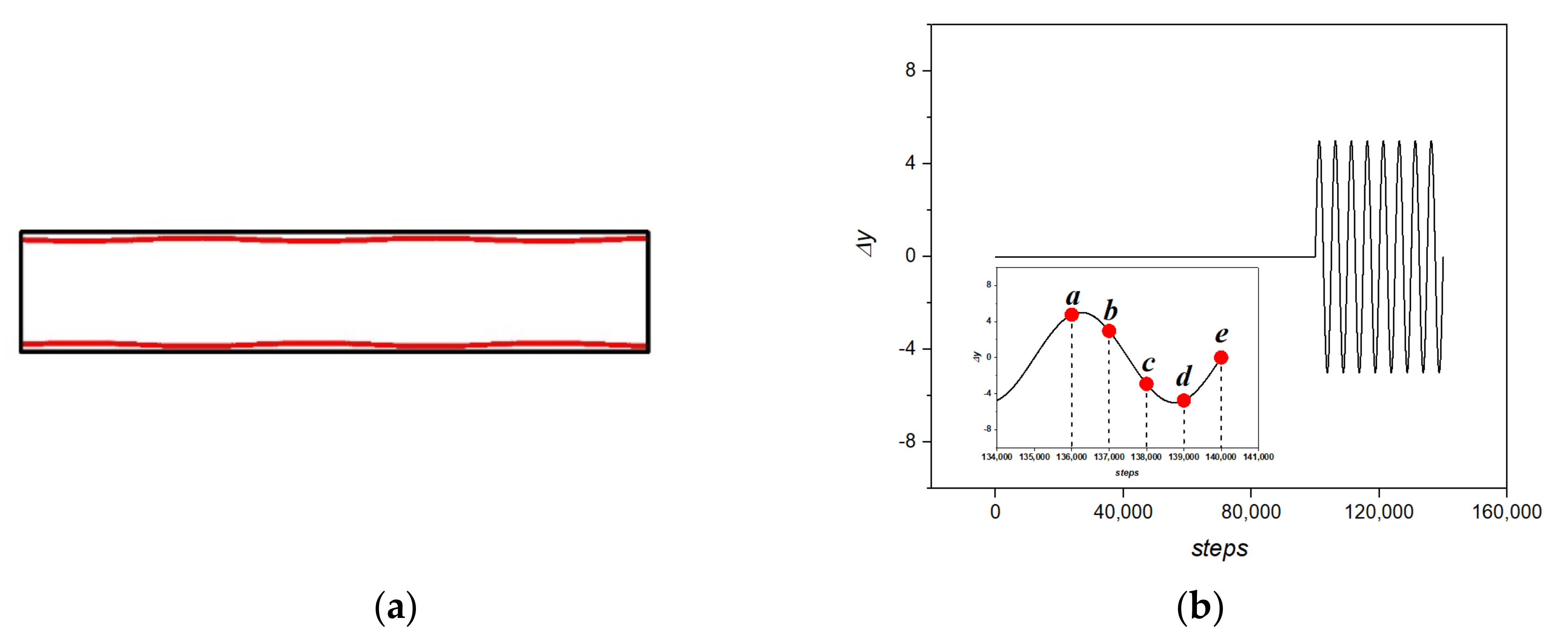
The parallel program environment of Message Passing Interface (MPI) was used to parallelize the LBM calculation code. In the calculation of static boundary problems, for example, the calculation resulted in Figure 4. In order to verify the applicability of this method in the pipeline flow with moving boundaries, the curved pipe wall model in Figure 7a was calculated. In Figure 7a, the scattered red points are the curved tube wall, and the solid black line is the calculation domain. The curved tube was approximated by a polyline segment connected by a series of points, and the movement of the points simulated the boundary motion of the curved tube. Before the simulation starts, we calculated the range of motion of these points. We set a rectangular area slightly larger than this range as the calculation domain. The advantage of this method is that the complexity of the model does not limit the computational domain. For a model of any shape, a larger rectangular area can contain the model, thereby converting the physical domain of a complex shape into a rectangular domain. The boundary influence is reflected in the flow field through boundary conditions.

The computational domain was [800, 3360], the interval was 1. Compared with the initial fit, the displacement of the pipe wall satisfied the displacement curve of Figure 7b. The displacement of a single pipe wall was equal, and the upper and lower pipe walls remained symmetrical. In the calculation, the incoming flow velocity was maintained at 0.08, the initial Re was 1000, and the inlet position of the lower pipe wall was 50.5 at the initial time. 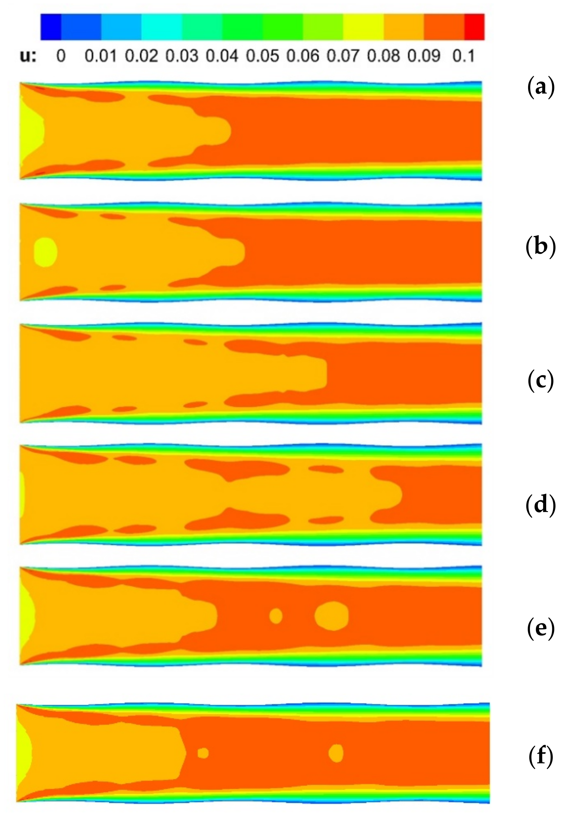As shown in Figure 7b, when the number of calculation steps exceeded 100,000, the displacement started with a sine function. The displacement period was 5000, and a total of eight periods were calculated. In the last displacement period, five equidistant monitoring points were selected. The flow field is shown in Figure 8.

In the inset in Figure 7b, the red dots are the monitoring points at five moments. Figure 8a–f shows the flow fields corresponding to these five detection points, and (f) is the final field with a static boundary. We kept the legend in Figure 8 consistent. It can be seen from Figure 7b that the pipe diameters of the monitoring points (a)~(d) gradually increased, and there were two complicated flow phenomena: inside the pipe, due to the increase in pipe diameter, the velocity decreased; the pipe entrance, due to the constant incoming flow velocity, the flow rate near the inlet increased and the velocity increased. Therefore, the yellow area at the entrance decreased, the light orange area increased, and the dark orange area decreased. In the scale, the speed values represented by the three colors increased sequentially. The flow field results conformed to the flow state. At times (d) and (f), the pipe wall was at the same position, and the flow field was different, indicating that the influence of pipe wall movement on the flow field was calculated. The difference was small, indicating that the impact of pipe wall movement was relatively small compared to the impact of the incoming flow. The flow field results conformed to the flow state, with no abnormal state, and the calculation results were good, showing this method’s applicability to the problem of moving pipeline flow.

5.4. Parallel Speedup and Efficiency

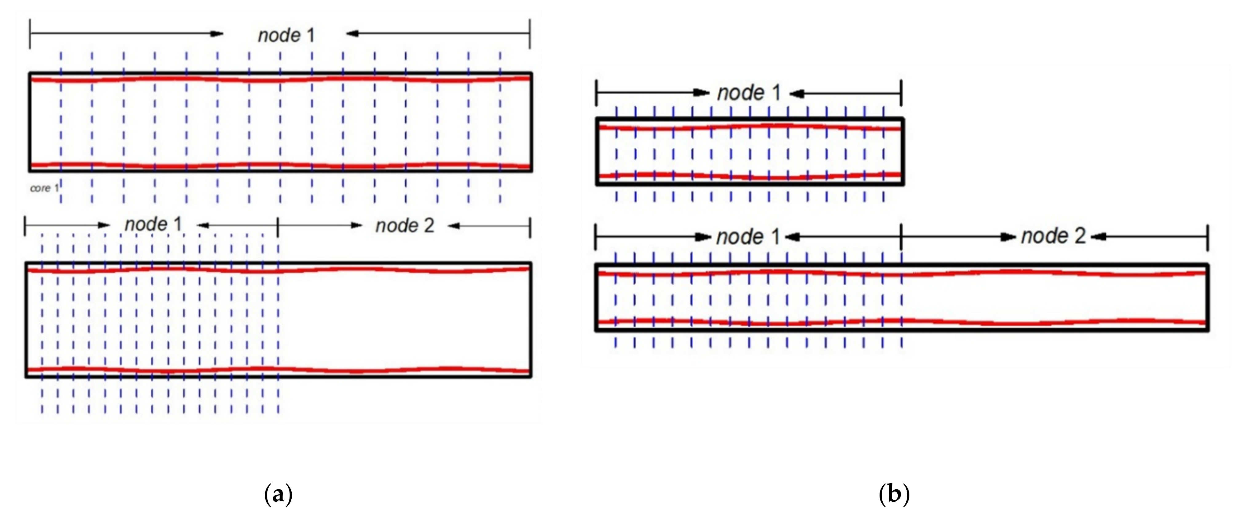
This article tested two kinds of parallel performance: keeping the overall task volume unchanged and increasing the number of computing cores; keeping the task volume of a single node unchanged and increasing the overall task volume. Figure 9 shows two kinds of parallel tests, a schematic diagram of a single node and two cores. In the first type of parallel test, the number of usable cores was limited by the computing domain. There was a minimum computing time, which predicted the computing time of a single task under the given computing resources. In the second type of parallel test, the ratio of communication time between cores in the total task was mainly tested, and the maximum calculation scale of the task was predicted.

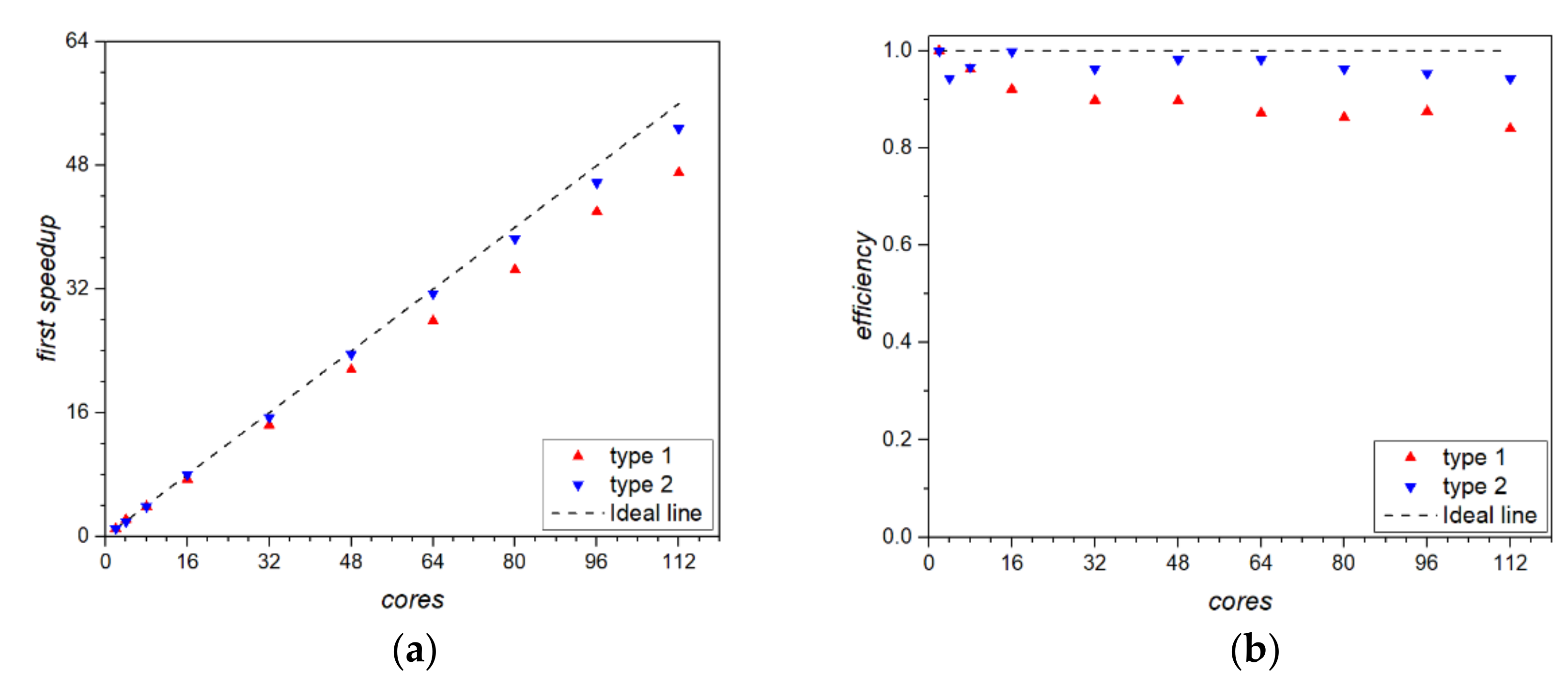
In the first parallel, due to the particularity of mesh generation, only the calculation time of the flow field calculation was tested, as shown in Figure 10. Two test results are given: type 1, the number of grids was 1680 × 400, the solid number was 3360; type 2, the number of grids was 3360 × 800, the solid number was 6720. It can be seen from Figure 10 that as the number of cores increased, the result of the first speedup ratio was close to the ideal speedup ratio. The number of grids and solid scattered points had little effect. In the 112 cores of the seven nodes tested, when the number of cores exceeded 16 cores, as the number of cores increased, the efficiency drop was small, basically staying above 80%. More grids had better efficiency. This shows that in the pipeline flow problem with moving boundaries, when the calculation scale is small, there is a good parallel effect.

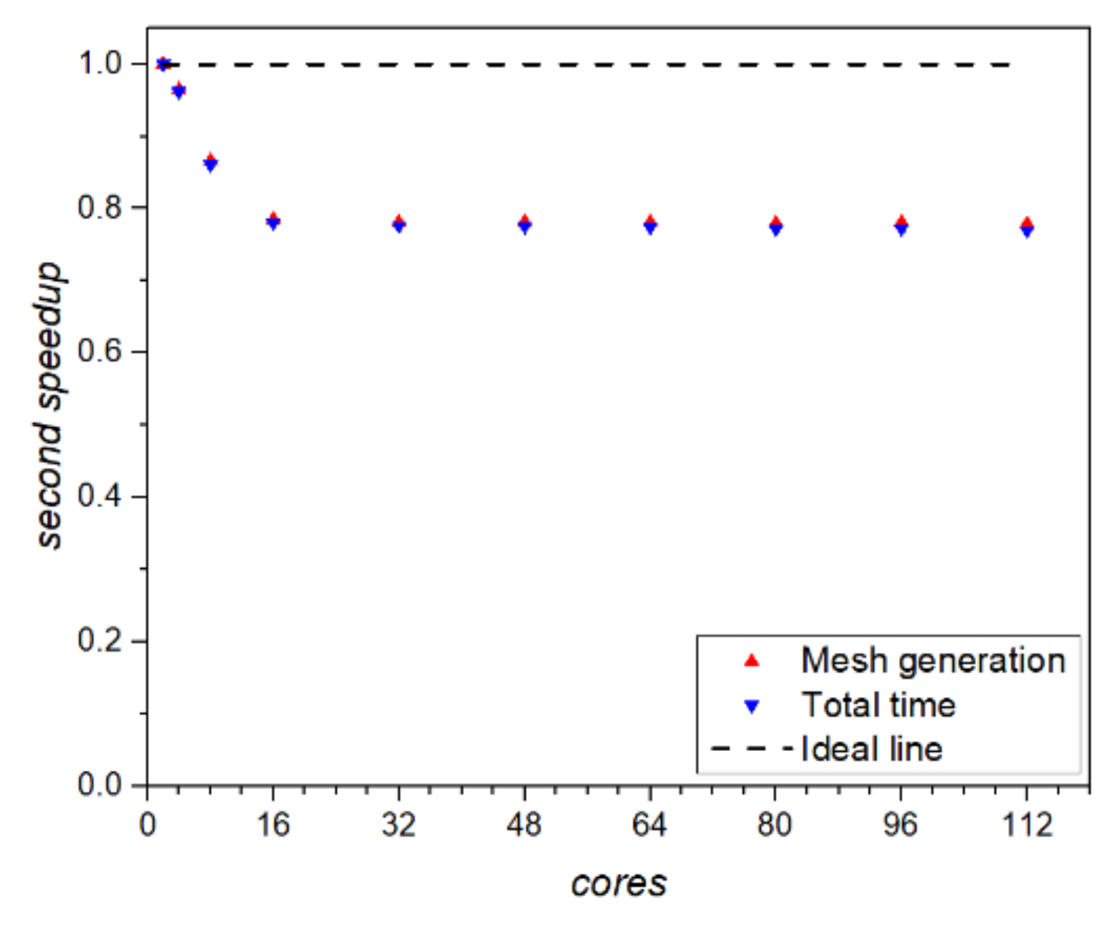
Figure 9b shows that while keeping the calculation amount of a single core unchanged, increasing the number of cores will increase the number of grids and the number of solid scattered points simultaneously. This means that when the calculation scale is increased, the resolution of the solid boundary will not be reduced, which is suitable for calculating complex boundaries. In this paper, the number of solid scattered points was allocated according to the number of cores before the mesh generation stage. During the mesh generation process, data communication between different cores was not required. It can be seen from Figure 11 that the acceleration result of the total time was close to the mesh generation. The results show that in the program, the proportion of communication was tiny, and the impact can be ignored, which is suitable for large-scale parallel calculations.

In calculating the moving boundary problem, as the solid boundary moves, the mesh generation step needs to be repeated, which will cause a huge computational overhead. Suppose only the number of grids is allocated according to the number of cores. In that case, the ideal speedup ratio of the mesh generation is a linear speedup ratio, i.e., the actual speedup multiple is close to the number of cores. In this paper, the number of solid grids was allocated simultaneously, significantly reducing the time overhead of mesh generation, thereby reducing the overall calculation time. Since this method is suitable for the moving boundary problem of the pipeline model, it can be applied to the fluid–solid coupling problem of blood vessels in future research.

6. Conclusions

This paper discussed the D2G9 method suitable for incompressible fluid calculation in LBM and analyzed the unified boundary method suitable for processing the boundary of complex curved surfaces. Considering the unknown distribution function when the grid point type changes in the moving boundary, this situation was supplemented and corrected. A parallel optimization strategy was proposed for a specific type of boundary model. Numerical simulations of the static cylinder and moving cylinder were carried out. The drag coefficient and vortex shedding frequency were calculated when the flow field was stable in the flow around a cylinder. The results of comparison with the results of existing researchers were consistent. In the simulation of the moving cylinder, the comparison of the flow field and the three parameters verified the accuracy of the simulation of the moving boundary problem. In a pipe flow with a moving pipe wall, the flow field results satisfied the flow law, and the influence of the moving boundary on the flow field was calculated clearly. Using MPI to parallelize the LBM calculation code, we tested two different parallel speedups. By allocating solid scattered points, the calculation time of mesh generation was shortened, and the overall parallel performance was improved. The first speedup ratio of the flow field calculation was basically close to the ideal speedup ratio, and the efficiency reached more than 80% at 112 cores. The second speedup ratio indicated that the proportion of communication in the program was tiny and suitable for large-scale parallel computing. Since this method is suitable for the moving boundary problem of the pipeline model, it can be applied to the FS problem of blood vessels in future research.