
Comparison of DFN Modelled Microfracture Systems with Petrophysical Data in Excavation Damaged Zone


1
Department of Civil Engineering, Aalto University School of Engineering, 02150 Espoo, Finland
2
Department of Engineering Geology and Geotechnics, Budapest University of Technology and Economics, 1111 Budapest, Hungary
3
Department of Mineralogy, Geochemistry and Petrology, University of Szeged, 6720 Szeged, Hungary
4
Department of Applied Mechanics, RISE Research Institutes of Sweden, 501 15 Borås, Sweden
*
Author to whom correspondence should be addressed.
Appl. Sci. 2021, 11(7), 2899; https://doi.org/10.3390/app11072899
Submission received: 28 February 2021
/
Revised: 15 March 2021
/
Accepted: 16 March 2021
/
Published: 24 March 2021
(This article belongs to the Special Issue Fractured Reservoirs)
Abstract
:Featured Application
Deep geological disposal of spent nuclear fuel.
Abstract
Physical and petrographic properties of drill core specimens were determined as a part of investigations into excavation damage in the dedicated study area in the ONKALO® research facility in Olkiluoto, Western Finland. Microfractures in 16 specimens from two drillholes were analysed and used as a basis for fractal geometry-based discrete fracture network (DFN) modelling. It was concluded that the difference in resistivity between pegmatoid granite (PGR) and veined gneiss (VGN) specimens of similar porosity was likely due to differences in the types of microfractures. This hypothesis was confirmed from microfracture analysis and simulation: fractures in gneiss were short and mostly in one preferred orientation, whereas the fractures in granite were longer and had two preferred orientations. This may be due to microstructure differences of the rock types or could suggests that gneiss and granite may suffer different types of excavation damage. No dependencies on depth from the excavated surface were observed in the geometric parameters of the microfractures. This suggests that the excavation damaged zone cannot be identified based on the changes in the parameters of the microfracture networks, and that the disturbed layer observed by geophysical methods may be caused by macro-scale fractures.
1. Introduction
Posiva Oy is responsible for the final disposal of the spent nuclear fuel of its owners Teollisuuden Voima Oy and Fortum Power & Heat Oy. As part of the disposal process, investigations have been carried out in the ONKALO® research facility in Olkiluoto, Western Finland. The chosen disposal method is deep geological disposal with multiple-barriers method KBS-3, originally developed by the Swedish Nuclear Fuel and Waste Management Company SKB, and more precisely its vertical variant KBS-3V. Spent fuel will be isolated from the environment with multiple engineered barriers; the fuel pellet, the fuel rod, a cast iron canister insert, a copper overpack, bentonite buffer, tunnel backfill, and finally several hundred metres of bedrock. The disposal method is described in Posiva Working Report 2012-66 [1]. This study is a part of the extensive on-going investigations of the excavation damaged zone caused by the drill and blast excavation method in access and deposition tunnels. Other studies of the EDZ in the context of nuclear waste disposal have been undertaken elsewhere, e.g., Ericsson et al. [2].
1.1. Excavation Damaged Zone Investigations in ONKALO®, Olkiluoto, Finland
Transport of radionuclides with water in fractured bedrock has been identified as one of the key risks to the environment related to the final disposal [3]. Excavation of the deposition and access tunnels with the drill and blast method causes damage to the surrounding rock mass, seen as the excavation damaged zone (EDZ). Characterisation of the EDZ is necessary for understanding the fluid transport properties of the damaged rock mass near the excavation profile of the tunnels.
Posiva committed a set of research works in ONK-TKU-3620 between 2012 and 2018 to characterise EDZ [4]. Research work consisted of geological, petrophysical, and rock mechanical studies and modelling. This study focuses on the discrete fracture network (DFN) analysis of drill core specimens from the EDZ study area in ONK-TKU-3620 [5] and the relationship between observed fracturing and measured petrophysical [6] and mechanical properties [7]. Specifically, the focus is on the network of micro and macro fractures potentially induced by the excavation, as opposed to pre-existing natural fracture systems.
1.2. Research Site
The excavation damaged zone study area in ONK-TKU-3620 is located at a depth of approximately 345 m along the ONKALO® access tunnel (Figure 1). ONK-TKU-3620 is approximately 50 m long by 10 m wide, oriented north–south and tilted upwards at a 5% angle [3]. The south end of the study area is dominated by gneissic specimens, mostly veined gneiss (VGN) with some inclusions of diatexitic gneiss (DGN). The north end of the study area consists mainly of pegmatoid granite (PGR) [8]. Based on the 3-D lithological model of Koittola [8], the gneissic rocks make up approximately 63% of the volume, whereas the pegmatoids account for the remaining 37%. The rock mass in the study area in general was considered structurally sound, with only minor natural fracturing [8], making it suitable for studying excavation-induced damage. A lithological model of the study area, the location of the study area in ONK-TKU-3620, all drillholes in the study area, and the locations of the drill holes sampled in this investigation are shown in Figure 2.
2. Materials and Methods
This study considered 16 specimens from two of the vertical drill holes (Set 1a, purple colour) shown in Figure 2. Specimens were selected based on four key criteria [6]:
- Specimens should be from as close to the tunnel floor as possible to capture the excavation damage effect.
- Specimens should represent the dominant rock types as well as possible.
- The distribution of rock types should represent the geology of the study area.
- Specimens from each hole should create a sequence as uniform as possible (ideally with no large fractures or core loss in between).
Rock types present in the specimens are veined gneiss (39 pcs, 49%), diatexitic gneiss (13 pcs, 16%), and pegmatoid granite (28 pcs, 35%). Gneissic specimens were cored such that the foliation plane was either approximately perpendicular or parallel to the specimen axis. Pegmatoid was assumed to have an isotropic material structure. Best sequences of veined gneiss (10 pcs, VGN) and pegmatoid granite (10 pcs, PGR) were selected for specimen Set 1a, bearing in mind the geological representativeness. The top depths of the gneissic specimens span a range from 0.07 to 0.77 m, and pegmatoids from 0.06 to 0.76 m from the excavated surface.
2.1. Specimen Preparation
Specimens that had a nominal diameter of 68 mm were cut into lengths of approximately 50 mm at the Geological Survey of Finland (GTK). When necessary, the ends of the specimens were ground to be smooth. Further preparations were done by SP Technical Research Institute of Sweden (since renamed RISE) when seen necessary for wave velocity measurements.
To get a better estimate of the physical properties of the rock mass in situ, all specimens were saturated in diluted saline water collected from ONKALO® instead of typical tap or distilled water. The ONKALO® water was diluted with ion-exchanged water to an electrical conductivity value of approximately 1240 mS/m, corresponding to typical measured salinity values at the site, and a total dissolved solids (TDS) content of approximately 7.56 g/L [9]. Specimens were fully submerged in the saturation water at normal temperature and pressure conditions for a period of at least two weeks to ensure full saturation.
2.2. Petrographic Description
To get an idea of the typical compositions of the studied granite and gneiss, petrographic analysis was performed [5]. At the gneiss specimen, biotite defines the foliation of the rock. The idiomorphic biotite grains contain elongated isomorphic opaque minerals and zircon in a large number. Besides biotite, the gneiss contains feldspars and quartz as major components. The plagioclase feldspar grains have polysynthetic twins. Alkali feldspars often show tartan twins, characteristic of microcline and a few myrmekitic grains can be observed in the thin sections. Quartz grains display signs of dynamic recrystallization, developed probably due to grain boundary migration. The potassium feldspar, microcline grains show tartan twinning and also show perthitic features in the thin sections. The metamorphic index minerals in the studied gneiss are kyanite sillimanite and garnet.
In the granite specimen, feldspars and quartz are also dominant. Plagioclase feldspar, which is sometimes sericitic, microcline, and also perthite, can be obtained in the thin sections. It seems like grain–boundary migration occurred in the quartz clasts. Rarely, myrmekite can be found in the thin sections. The granite contains idiomorphic biotite, but its quantity is not enough to define foliation. Muscovite also occurs in the granite specimen.
2.3. Petrophysical Testing
Extensive petrophysical testing was conducted on the specimens. In this section, the testing methods for density, porosity, resistivity, relative permittivity and seismic wave velocities are briefly described.
2.3.1. Density and Porosity
Density and porosity were determined by two individual operators: The Geological Survey of Finland (GTK) and SP Technical Research Institute of Sweden. The method used was based on Archimedes’ principle, and uses three weighings of the specimens (dry in air, saturated in air, saturated in water) to determine the pore space and bulk volumes, which are then used to calculate the density and porosity when the density of the saturation fluid is known.
2.3.2. Resistivity and Relative Permittivity
The electrical resistivity of the specimens was measured by GTK using their proprietary galvanic 2-point measurement system with wet electrodes and saturated specimens. In short, the specimen was placed in a serial circuit with a known resistor, and current was measured over the system. Measurements were done at three frequencies: 0.1, 10, and 500 Hz.
Relative dielectric permittivity was measured using an Adek Percometer v.7 with a surface probe. Both the top and the bottom of the specimen were measured three times, and these were averaged out in the calculation, and corrected with a standard specimen measured before and after each specimen, to yield the permittivity estimate.
2.3.3. Seismic P- and S-Wave Velocities
P-wave velocity was measured by both GTK and SP, S-wave velocity by SP only. All velocities were measured on unloaded specimens in the axial direction. The P-wave velocity measurement at GTK was done using sonar elements with a pulse central frequency of approximately 1 MHz. The saturated specimens were measured submerged at normal temperature and pressure.
P- and S-wave velocity measurements carried out by SP were conducted according to ASTM International standard D 2845-00 [10]. The system used for velocity measurements was a GCTS ULT-100 ultrasonic pulse generator and sampling device with heavy-duty 76-mm-diameter steel plates with integrated piezoelectric crystals from GCTS. The transducers had a resonant frequency of 200 kHz and included both P- and S-crystals. The pulse used was a 130 V/5 µs square wave generated with the ULT-100; see Jacobsson et al. [7] for details.
By assuming the rock to be a homogeneous isotropic material with a linear elastic response it was possible to determine the Poisson’s ratio from the P-and S-wave velocity values as:
where υ is Poisson’s ratio, and Vp and Vs are the P- and S-wave velocities, respectively. Young’s modulus can be calculated as:
2.4. Fracture Network Simulation
Microfracture porosity is a main contributor to fluid flow in intact crystalline rocks. Characterization of the microfracture geometry can be achieved by modelling the fracture system’s characteristic geometric data: interconnectivity, openness, and density of the microfracture systems. There are three major approaches to modelling the hydraulic properties: An (1) equivalent continuum, (2) DFN, or (3) hybrid models combining an equivalent continuum and DFN [5,11,12,13].
DFN models are founded on the assumption that fluid flow behaviour can be predicted from the fracture geometry data of individual fractures [14]. The basis of the generated realizations of fracture networks is their spatial statistics, which can be measured. The realizations have the same spatial properties as the analysed fracture network. The approach taken here has been successfully used before, including in the context of radioactive waste disposal [15,16,17]
2.4.1. Geometric Parameters
Individual fractures are spatially finite and can be interpreted as multiply bent two-dimensional surfaces, which can be approximated as planes [18,19,20]. They appear circular in isotropic rocks and form ellipsoids (penny shape) in anisotropic rocks [21]. The length and aperture parameters define the size of the fracture. Natural fracture networks generated under a specific stress field show fractal behaviour, e.g., [22,23,24]. They are self-similar and self-affine [25], which allows scaling.
It is generally agreed that the size distribution of fracture lengths is asymmetric, with small fractures significantly outnumbering larger ones [24]. It can be estimated that the relative number of short to long fractures is an invariant of the scale [24]. The length distribution of fractures in a fracture network is commonly described as:
where N is the number of fractures longer than L, F is a constant dependent on the size of the specimen, and E* is the fracture length index [26,27]. The fracture length index E* characterizes the distribution of the lengths of a given fracture set: The greater the absolute value of E*, the more short fractures are present.
Fracture length and aperture are often considered to be linearly correlated, e.g., [22,28,29]. Aperture A can be defined as:
where l is the fracture length and a and B are constants [29]. Constant a describes the ratio of the maximum aperture/length and has been estimated to be between 2.1 × 10⁻⁴ and 8.2 × 10⁻³ [29]. B describes the aperture of fractures with zero length and should thus be zero but can obtain non-zero values since the constants are typically defined using linear regression.
The spatial density of fractures scales due to the fractal nature of the fracture systems and can be estimated using box-counting [22,25,30]. Here, the studied image is covered by boxes with varying sizes. Number N of boxes containing a part of the studied image is proportional to their size r as:
where D is a constant. For fractal images, D ≠ 1 and the fractal dimension Df can be estimated as the slope of log (N(r)) against log(r) as:
The fractal dimension is a quantitative parameter of a fracture network, which defines the spatial density of fractures.
Strike and dip define the orientation of an individual fracture, and the orientation of a group of fractures is approximated with a mathematical distribution generated from the strike and dip values of individual fractures.
2.4.2. Input Data Acquisition
For the microfracture network analysis, 5-mm-thick disks were cut from the 16 specimens perpendicular to the drillhole axis, and polished after impregnation with UV fluorescent epoxy. The specimens were then illuminated with refracted UV light and photographed with an Olympus DP73 camera mounted on an Olympus BX41 microscope with 1.25× magnification. The microscope was used in reflected-light mode with a 100-Watt U-LH100HG mercury vapour lamp as the light source and an Olympus U-MWBV2 filter cube installed (excitation range between 400 and 440 nm).
Images were processed using the Trainable Weka Segmentation plug-in of the ImageJ-based Fiji environment [31], which allowed the images to be simplified and reduced to two types of pixels: fractures and host rock. Examples of a fluorescent image, segmented image, and then skeletonised image are shown in Figure 3. The images were further processed in MATLAB, and then geometric parameters of the microfracture networks were extracted from the images using an algorithm that was developed for this purpose (Figure 4). The algorithm detects the branch points of the intersecting fractures, and based on the dip of the fractures to a reference line, it divides them into separate linear objects. This allows the end and centre points of the individual fractures to be detected. Based on the data sets of these points, the algorithm calculates the length and orientation of the fractures. The geometric parameters of a fracture set, such as the fracture length index and fractal dimension, were then determined as shown in Section 2.4.1. A basic overview of the process workflow is shown in Figure 5.
2.4.3. Simulations with REPSIM Software
The extracted microfracture parameters were used as the basis for modelling of 10 m × 10 m × 10 m blocks of varying combinations of VGN and PGR. The approach is fractal geometry based and assumes that the (statistical distribution of) parameters of the larger blocks are equal to the parameters of the microfracture networks, i.e., that the system is scalable.
The modelling was done using a fractal geometry-based discrete fracture network (DFN) algorithm of the REPSIM software package [14]. The software generates fracture networks stochastically based on the statistical distribution of observed parameters. The input parameters required for each homogenous unit cube are:
- Fractal dimension for fracture centres for spatial density distribution.
- Parameters of the fracture length distribution;
- Lower and upper extreme fracture length;
- Aperture as a function of length [29]; and
- Strike and dip data.
Several runs of models were conducted with varying gneiss and granite contents, yielding the corresponding number of realisations of the model. The geometry of the models consisting of both gneiss and granite were built to simulate inclusions; accordingly, the granite cells were positioned in an ellipsoid-like shape in the centre of the modelled volume (Figure 6).
The simulations result in fracture networks that have the same spatial statistics as the input parameters. The generated fracture networks are equally probable realizations of the given stochastic distribution. The number of intersecting, thus connective, fracture groups and the size of these clusters can be detected from the results. It is also possible with REPSIM to visualize the generated fracture networks, as it is shown in Figure 7.
3. Results
This section focuses on the results of the fracture network analysis. Results of the petrophysical testing are only summarised in the extent needed for the comparisons.
3.1. Petrophysical Analysis
Key results of the petrophysical testing are presented here as descriptive statistics for specimens (Table 1). The smallest and largest observed densities were 2608 and 2748 kg/m3, respectively, with gneiss yielding on average slightly higher densities (mean value of 2732 kg/m3 vs. 2622 kg/m3 for PGR). The variance of the density values within rock types was small. Porosities ranged from 0.27% to 0.75%, with the mean values for VGN and PGR being practically identical.
Resistivities and relative permittivity values of the VGN specimens were significantly higher than those of the PGR. P-wave velocities of VGN were slightly lower than PGR on average (mean values of 5592 and 5800 m/s, respectively), while the observed ranges were very close to each other. The S-wave velocities of VGN were slightly lower than PGR on average (mean values of 3161 and 3263 m/s, respectively), while VGN showed a much higher variance. Young’s modulus shows a similarly high variance in VGN compared to PGR, but on average the stiffness of the rock types is similar (mean values of 69.0 and 70.4 GPa for VGN and PGR, respectively).
The measured values were compared to previous data from Olkiluoto (results prior to 2009 summarised in Aaltonen et al. [32]) when possible and found to be generally in good agreement. It must be noted that the sample sizes (N = 10 for both rock types) are small. More comprehensive petrophysical testing and analysis of specimens from the study area can be found in Kiuru [6].
3.2. Fractal Dimensions and Fracture Length Distribution
The determined fractal dimensions of the microfracture networks and fracture midpoints showed no dependence on the depth of the specimen from the study area surface. No significant variation in the values was observed. The fractal dimension of the fracture midpoints D clearly differentiates the different rock types (Figure 8).
Fracture length distribution parameters show more variance, but this was not systematic. No dependence on specimen depth could be observed. From these observations, EDZ cannot be identified based on the changes in the parameters of the microfracture networks. The results are summarised in Table 2.
3.3. DFN Simulations
The simulations showed systematically more fractures and more connected fractures in granite compared to gneiss. Fractures in the gneiss were predominantly short and mostly arranged into one preferred orientation (Figure 9a). Fractures in pegmatoid granite had two preferred orientations, and they were longer (Figure 9b). Both the number of large fracture clusters (>100 fractures), and the maximum number of fractures in one cluster increased linearly as the volumetric content of PGR increased. However, the total number of connected microfracture clusters was negligible in both rock types. The results are shown in Figure 10.
3.4. Comparison of Fracture Network Parameters and Petrophysical Data
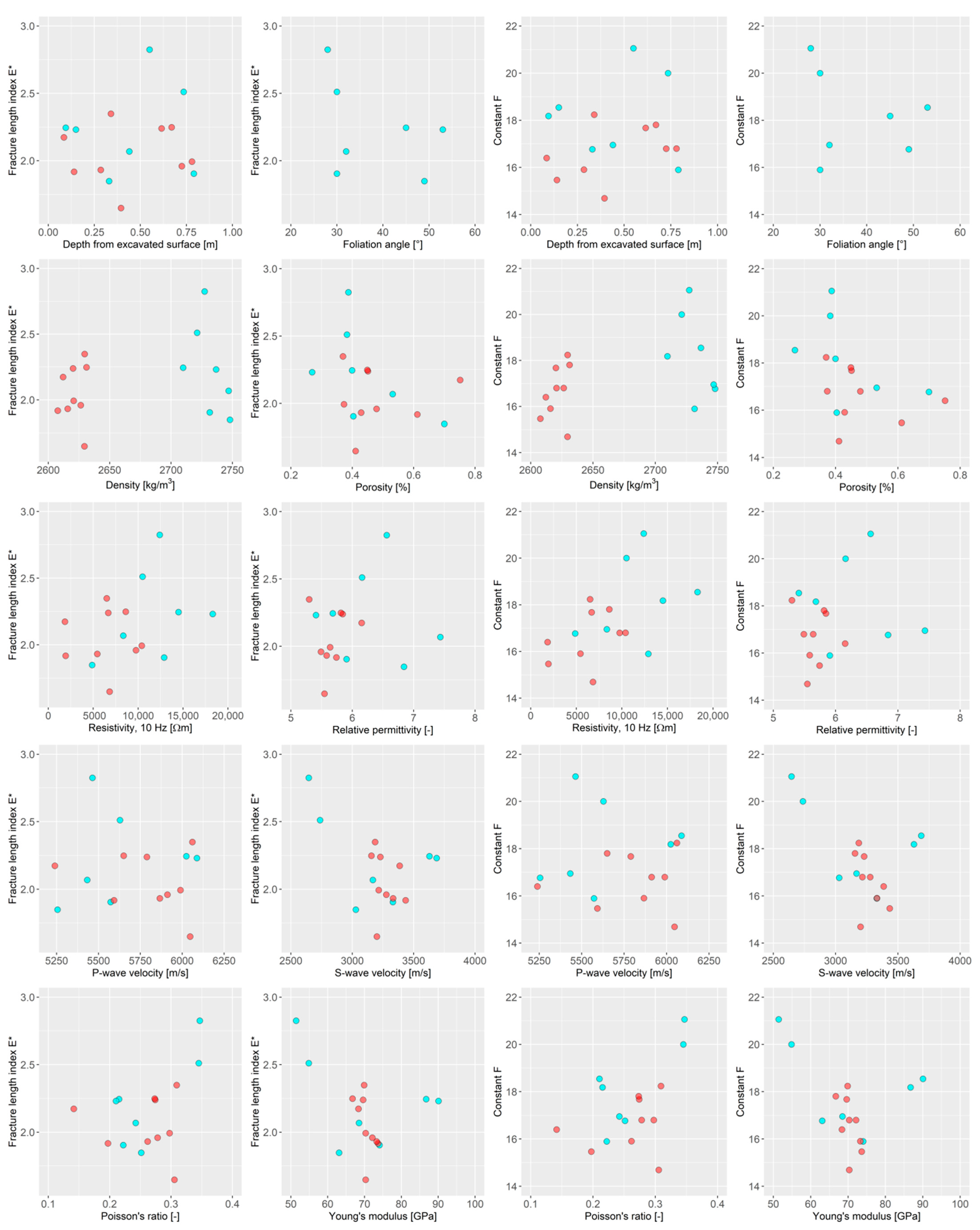
To study possible associations between the physical properties and fracture network parameters, cross plots of select variables were made. The fracture length index E*, the constant F, and the fractal dimensions of the system (Df) and as determined at fracture midpoints (D) were plotted against the specimen depth, foliation direction, density, porosity, resistivity, relative dielectric permittivity, P- and S-wave velocities, P/S-ratio, Poisson’s ratio, and Young’s modulus (Figure 11).
The fracture length index E* showed no clear association with the depth of the specimen or foliation direction. Density showed slightly higher values of E* in VGN as compared to PGR but no general trends. Porosity vs. fracture length showed a weak general negative trend, whereas resistivity vs. fracture length appeared to have a general positive trend. Relative dielectric permittivity showed a positive trend, except for two outliers in the data. The P- and S-wave velocities, P/S-ratio, Poisson’s ratio, and Young’s modulus showed no dependency on fracture length.
Interestingly, the constant F, which is only supposed to be a function of specimen size, showed a clear dependence on density and thus rock type. This observation could not be explained. F also showed similar trends for porosity, resistivity, and relative permittivity to fracture length. The rest of the parameters showed no trends. Neither Df nor D showed an association with specimen depth or foliation direction. Both separated the two rock types based on density. Df showed a more similar distribution of values, with gneiss showing large outlier values that granite was missing. D, on the other hand, showed clearly higher values for granite compared to gneiss.
Df versus porosity seemed to show a weak positive trend, whereas D showed no similar behaviour. Resistivity showed no trends, but relative permittivity had a negative trend for both Df and D. P- and S-wave velocities showed no clear trends, but the P/S-ratio and Poisson’s ratio seemed to have broad negative trends with respect to Df. The Young’s modulus did not appear to have a trend with respect to Df, and no trends appeared for any of the elasticity parameters with respect to D.
4. Discussion
Technical limitations introduce some bias into the study, e.g., the most damaged sections physically cannot be included in the specimens, meaning that no macro-scale fractures are present in the specimens. The specimens are typically required to be relatively intact, and as a result may not be representative of macro-scale EDZ.
Analysis of the geometric parameters from the prepared specimens should be a straightforward process with not much room for error, and the process remained systematic [13]. This means that fluorescent images were produced in fixed conditions (light, camera settings, possible post processing) before the segmentation to avoid biases. Considering the focus of the study is on the microfractures, it is possible that the preparation of the specimens has a disturbing effect.
The effect of drilling was studied by looking at a section that transects a specimen perpendicular to the drillhole axis. No difference in the microfracture network properties was found with respect to the distance from the specimen axis. This means that the effect of drilling was irrelevant to the studied problem. However, it must be noted that this test was limited to a single specimen, and for future studies more comprehensive testing might be in order.
Cutting and grinding the specimen ends might have an effect, but as cut and ground surfaces are always present their effect is impossible to distinguish. It is, however, likely that for similar specimens, the effect is similar and would therefore not affect the results within a specimen set to any significant degree.
The geometric parameters of the fracture network were only studied in sections taken in the x-y plane. Gneiss has an anisotropic structure, which may affect the results. However, the Olkiluoto gneiss has centimetre-scale variation in the foliation direction, which means the sections represent multiple orientations with respect to foliation.
The resistivity values varied approximately four to five times between the smallest and largest value for both the granite and gneiss, respectively. The resistivity value is sensitive to single “channels” of microcracks; thus, the orientation of microcracks in relation to the measurement direction is of importance. The microcracks and their orientations also affect the wave velocities but with a smaller impact. The fact that the specimens are fluid saturated could decrease the effect of microcracks for the P-wave velocity [33]. The porosity of the specimens is very small and was found to be practically isotropic in this context.
The modelling was limited to 5 models of varying compositions and 10 runs per model. For future work, the effect of the stress field on the orientation of formed fractures should be studied. Additional rock types would increase the understanding on the subject.
More fractures in total and more connected fracture clusters with more fractures per cluster in the simulations were observed in granite compared to gneiss. Based on the results, the number of larger micro fracture clusters and maximum number of fractures per cluster increases linearly with increasing volumetric granite content. It must be noted, however, that the fractal-based approach of the modelling assumes that the statistical distribution of the parameters remains the same regardless of scale.
Differences in the microfracture properties may either be natural or caused by drill and blast excavation. Differentiating the effect of fracturing from the effect of rock type, when the type of fracturing seems to depend on the rock type is tricky. The observed differences in the fracturing and electrical properties between the pegmatoid and gneissic specimens may suggest that pegmatoids are more prone to fracturing. Alternatively, it may also be that the natural heterogeneity of the gneissic specimens has an effect that exceeds the effect of excavation damage, disguising it.
5. Conclusions
The physical and mechanical properties of drill core specimens were determined as a part of investigations into excavation damage in the dedicated study area. Additionally, microfractures in 16 specimens were analysed and used as a basis for DFN modelling. Composition was analysed via thin sections and microfracture network properties via tinted epoxy impregnated rock disks with a MATLAB algorithm. The possible influence of drilling, cutting, grinding, and polishing on the specimens was considered and concluded not to affect the results of individual specimens to any significant degree.
There was a notable difference in resistivity between the pegmatoid and gneissic specimens, even though previous studies have shown that the resistivity distributions of Olkiluoto pegmatoids and veined and diatexitic gneisses are similar [6,32]. Furthermore, the observed differences in the resistivity of water-saturated specimens were found to be controlled mainly by differences in porosity [6]. As the observed porosities of the specimens did not differ significantly, the observed differences in the resistivities are likely due to differences in the rock matrix and the resulting differences in the type of microfractures, such as their orientation and following interconnectivity. This hypothesis was supported by the analysed thin sections and simulations: fractures in gneiss were short and mostly in one preferred orientation, likely controlled by foliation, whereas the fractures in granite were longer and had two preferred orientations. This suggests that gneiss and granite may suffer different types of excavation damage. A complementary or alternatively measure for the bulk porosity could be the microcrack porosity determined from mechanical testing [34].
In conclusion:
- The number of large microfracture clusters and maximum number of fractures per cluster increases linearly with increasing volumetric granite content.
- The total number of connected fracture clusters is negligible from the point of view of hydraulic conductivity in both rock types.
- No systematic changes in the geometric parameters of the microfracture networks were observed with respect to depth, while differences between gneiss and granite were observed.
- This suggests that excavation does not cause detectable perturbance of the intact crystalline rock’s microfracture porosity, i.e., that the excavation damaged zone cannot be identified based on changes in the parameters of the microfracture networks.
- The disturbed EDZ layer observed by geophysical methods may be caused by larger-scale fractures not present in the relatively intact specimens.
Author Contributions
Conceptualization, R.K., D.K. and L.J.; methodology, R.K., D.K., G.D. and L.J.; software, D.K. and G.D.; formal analysis, R.K. and D.K.; investigation, R.K., D.K. and L.J.; writing—original draft preparation, R.K. and D.K.; writing—review and editing, R.K., D.K., G.D. and L.J.; visualization, R.K. and D.K. All authors have read and agreed to the published version of the manuscript.
Funding
This research is based on work funded by Posiva Oy. This research was funded by the Academy of Finland, grant number 319798.
Institutional Review Board Statement
Not applicable.
Informed Consent Statement
Not applicable.
Data Availability Statement
Restrictions apply to the availability of these data. Data was obtained from Posiva Oy and are available in the cited working reports at www.posiva.fi (accessed on 1 February 2021) or from the authors with permission of Posiva Oy.
Acknowledgments
We would like to thank Posiva Oy for access to the data and the possibility to publish the results.
Conflicts of Interest
This research is based on work contracted by Posiva Oy. The views expressed are those of the authors and do not necessarily reflect those of Posiva Oy.
References
- Palomäki, J.; Ristimäki, L. (Eds.) Facility Description 2012; WR 2012-66; Posiva Oy: Eurajoki, Finland, 2013. [Google Scholar]
- Ericsson, L.O.; Thörn, J.; Christiansson, R.; Lehtimäki, T.; Ittner, H.; Hansson, K.; Butron, C.; Sigurdsson, O.; Kinnbom, P. A Demonstration Project on Controlling and Verifying the Excavation-Damaged Zone. Experience from the Äspö Hard Rock Laboratory; SKB R-14–30; Swedish Nuclear Waste and Management Co.: Stockholm, Sweden, 2015. [Google Scholar]
- Mustonen, S.; Norokallio, J.; Mellanen, S.; Lehtimäki, T.; Heikkinen, E. EDZ09 Project and Related EDZ Studies in ONKALO 2008–2010; Working Report 2010–2027; Posiva Oy: Eurajoki, Finland, 2010. [Google Scholar]
- Kiuru, R.; Heikkinen, E.; Jacobsson, L.; Kovács, D. EDZ Study Area in ONK-TKU-3620: Petrophysical, Rock Mechanics and Petrographic Testing and Analysis Conducted on Drill Core Specimens between 2014 and 2016; WR 2017–56; Posiva Oy: Eurajoki, Finland, 2019. [Google Scholar]
- Kovács, D.; Dabi, G.M.; Tóth, T.; Jacobsson, L.; Kiuru, R. EDZ Study Area in ONK-TKU-3620: Discrete Fracture Network Based Modelling of Microcrack Systems in Drill Core Specimens and Comparisons with Petrophysical Measurements; WR 2016–56; Posiva Oy: Eurajoki, Finland, 2019. [Google Scholar]
- Kiuru, R. EDZ Study Area in ONK-TKU-3620: Association Analysis of Petrophysical and Rock Mechanics Data; WR 2016–42; Posiva Oy: Eurajoki, Finland, 2019. [Google Scholar]
- Jacobsson, L.; Kjell, G.; Brander, L.; Kiuru, R. EDZ Study Area in ONK-TKU-3620: Determination of Seismic Wave Velocities at Six Load Levels, Petrophysical and Rock Mechanical Properties of Drill Core Specimens; WR 2016–57; Posiva Oy: Eurajoki, Finland, 2019. [Google Scholar]
- Koittola, N. Geological 3D Model of the Investigation Niche in ONKALO, Olkiluoto, Southwestern Finland; WR 2014–35; Posiva Oy: Eurajoki, Finland, 2014. [Google Scholar]
- Ruotsalainen, P.; Ahokas, H.; Heikkinen, E.; Lindh, J.; Nummela, J. Groundwater salinity at the Olkiluoto site Groundwater salinity at the Olkiluoto site; WR 2000–26; Posiva Oy: Eurajoki, Finland, 2000. [Google Scholar]
- ASTM. D 2845–00 (Reapproved 2004). Standard Test Method for Laboratory Determination of Pulse Velocities and Ultrasonic Elastic Constants of Rock; ASTM International: West Conshohocken, PA, USA, 2004. [Google Scholar]
- Dershowitz, W.S.; Einstein, H.H. Characterizing rock joint geometry with joint system models. Rock Mech. Rock Eng. 1988, 21, 21–51. [Google Scholar] [CrossRef]
- Long, J.C.S. (Ed.) Rock Fractures and Fluid Flow: Contemporary Understanding and Applications; National Academy Press: Washington, DC, USA, 1996; 551p. [Google Scholar]
- Kovacs, D.; Dabi, G.; Vásárhelyi, B. Image processing for fractal geometry-based discrete fracture network modeling input data: A methodological approach. Cent. Eur. Geol. 2018. [Google Scholar] [CrossRef]
- Tóth, T.M.; HoLLóS, C.S.; Szűcs, É.; Schubert, F. Conceptual fracture network model of the crystalline basement of the Szeghalom Dome (Pannonian Basin, SE Hungary). Acta Geol. Hung. 2004, 47, 19–34. [Google Scholar] [CrossRef]
- Bauer, M.M.; Tóth, T. Characterization and DFN modelling of the fracture network in a Mesozoic karst reservoir: Gomba oilfield, Paleogene Basin, Central Hungary. J. Pet. Geol. 2017, 40, 319–334. [Google Scholar] [CrossRef]
- Tóth, M.T. Determination of geometric parameters of fracture networks using 1D data. J. Struct. Geol. 2010, 32, 878–885. [Google Scholar] [CrossRef]
- Tóth, T.M. Fracture network characterization using 1D and 2D data of the Mórágy Granite body, Southern Hungary. J. Struct. Geol. 2018, 113, 176–187. [Google Scholar] [CrossRef] [Green Version]
- Snow, D.T. A Parallel Plate Model of Fractured Permeable Media. Ph.D. Thesis, University of California, Berkeley, CA, USA, 1965; p. 331. [Google Scholar]
- Chiles, J.; De Marsily, G. Models of fracture Systems. In Flow and Contaminant Transport in Fractured Rock; Bear, J., Tsang, C.F., De Marsily, G., Eds.; Academic Press, INC: Cambridge, MA, USA, 1993. [Google Scholar]
- Mardia, K.; Nyirongo, V.; Walder, A.; Xu, C.; Dowd, P.; Fowell, R.; Kent, J. Markov chain Monte Carlo implementation of rock fracture modelling. Math. Geol. 2007, 39, 355–381. [Google Scholar] [CrossRef]
- Twiss, R.J.; Moores, E. Structural Geology; W H Freeman: New York, NY, USA, 1992; p. 532. [Google Scholar]
- Barton, C.C.; Larsen, E. Fractal geometry of two-dimensional fracture networks at Yucca Mountain, Southwestern Nevada. In Proceedings of the International Symposium on Fundamentals of Rock Joints; Stephanson, O., Ed.; Centek: Lulea, Sweden, 1985; pp. 77–84. [Google Scholar]
- Roberts, S.; Sanderson, D.J.; Gumiel, P. Fractal analysis of the Sn–W mineralization from central Iberia: Insights into the role of fracture connectivity in the formation of an ore deposit. Econ. Geol. 1998, 93, 360–365. [Google Scholar] [CrossRef]
- Tóth, T.M.; Vass, I. Relationship between the geometric parameters of rock fractures, the size of percolation clusters and REV. J. Math. Geosci. 2011, 43, 75–97. [Google Scholar] [CrossRef]
- Mandelbrot, B.B. The Fractal Geometry of Nature; Freeman: New York, NY, USA, 1983; 468p. [Google Scholar]
- Yielding, G.; Walsh, J.J.; Watterson, J. The prediction of small-scale faulting in reservoirs. First Break 1992, 10, 449–460. [Google Scholar] [CrossRef]
- Min, K.; Jing, L.; Stephansson, O. Determining the equivalent permeability tensor for fractured rock masses using a stochastic REV approach: Method and application to the field data from Sellafield, UK. Hydrogeol. J. 2004, 12, 497–510. [Google Scholar] [CrossRef]
- Pollard, D.; Segall, P. Theoretical displacements and stresses near fractures in rock: With application to faults, joints, veins, dikes and solution surfaces. In Fracture Mechanics of Rock; Atkinson, B., Ed.; Academic Press: London, UK, 1987. [Google Scholar]
- Vermilye, J.M.; Scholz, C.H. Relation between vein length and aperture. J. Struct. Geol. 1995, 17, 423–434. [Google Scholar] [CrossRef]
- Barton, C.C. Fractal analysis of scaling and spatial clustering of fractures. In Fractals in the Earth Sciences; Barton, C.C., La Pointe, P.R., Eds.; Plenum Press: New York, NY, USA, 1995; p. 168. [Google Scholar]
- Arganda-Carreras, I.; Kaynig, V.; Schindelin, J.; Cardona, A.; Seung, H.S. Trainable Weka Segmentation: A Machine Learning Tool for Microscopy Image Segmentation. Bioinformatic 2014, 33, 2424–2426. [Google Scholar] [CrossRef] [PubMed]
- Aaltonen, I.; Heikkinen, E.; Paulamäki, S.; Säävuori, H.; Vuoriainen, S.; Öhman, I. Summary of Petrophysical Analysis of Olkiluoto Core Samples 1990–2008; WR 2009–11; Posiva Oy: Eurajoki, Finland, 2009. [Google Scholar]
- Biot, M.A. Theory of propagation of elastic waves in fluid-saturated porous solid: II Hihger frequency range. J. Acoust. Soc. Am. 1956, 28, 179–191. [Google Scholar] [CrossRef]
- Jacobsson, L.; Flansbjer, M.; Christiansson, R.; Jansson, T. Measurement of micro crack volume in low porosity crystalline rock. In Proceedings of the 11th Congress of the International Society for Rock Mechanics, Lisbon, Portugal, 9–13 July 2007. [Google Scholar]
Figure 1.
Location of ONK-TKU-3620 in ONKALO® marked with a red circle. Viewed from the south. Image courtesy of Posiva Oy.
Figure 1.
Location of ONK-TKU-3620 in ONKALO® marked with a red circle. Viewed from the south. Image courtesy of Posiva Oy.

Figure 2.
Location of the excavation damaged zone study area in ONK-TKU-3620 in ONKALO® and a blow-up of the lithological model of the study area and drillholes in the study area. Red volume is pegmatoid granite, light blue volume is veined gneiss. Drillholes sampled in this study are marked in purple, other drillholes are marked in grey. Dimensions are in metres.
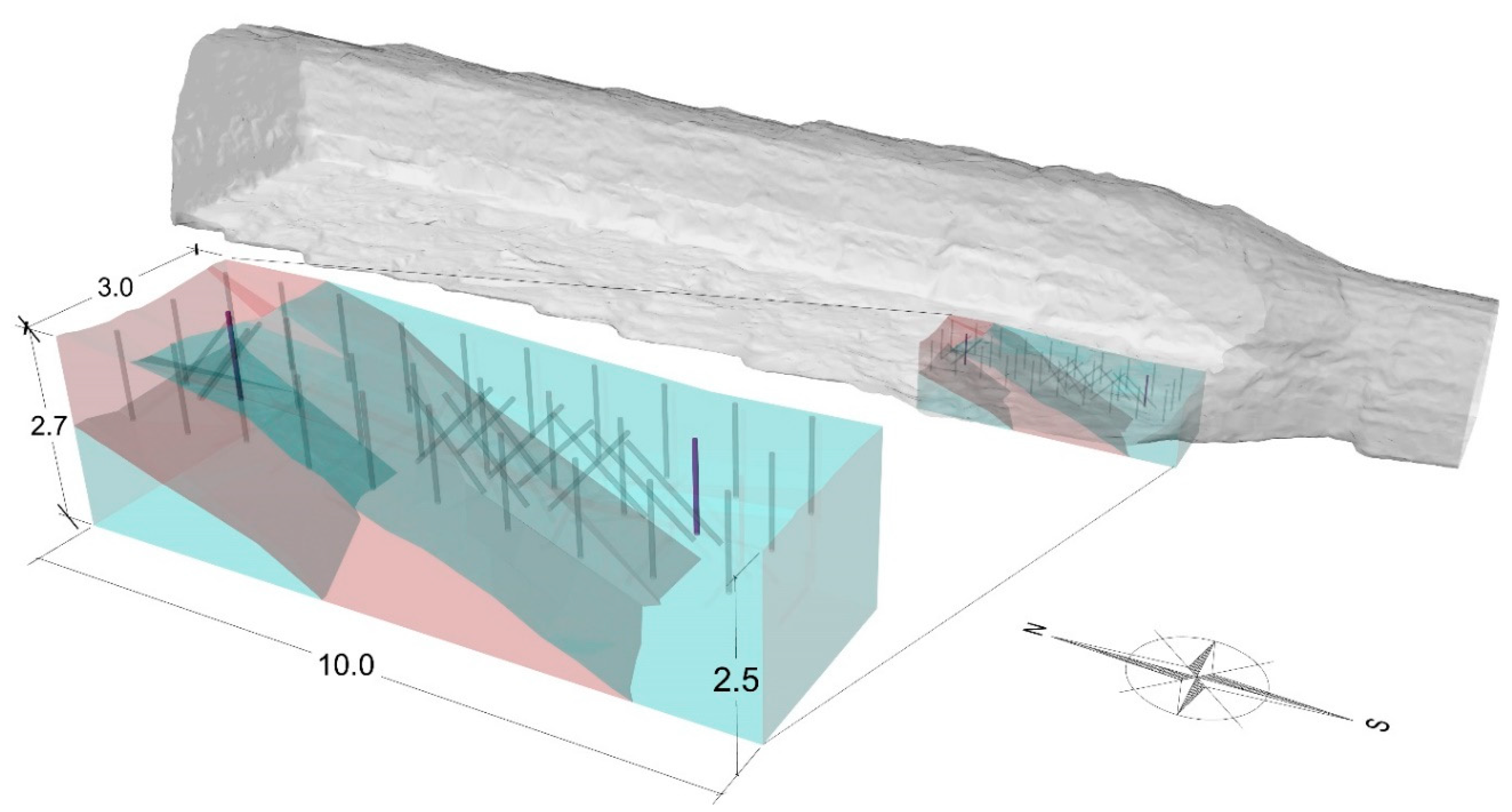
Figure 3.
Example of (a) a fluorescent image of the microfracture network; (b) the resulting segmented image; and (c) a close up of the skeletonised image. Adapted from Kovács et al. [5,13].
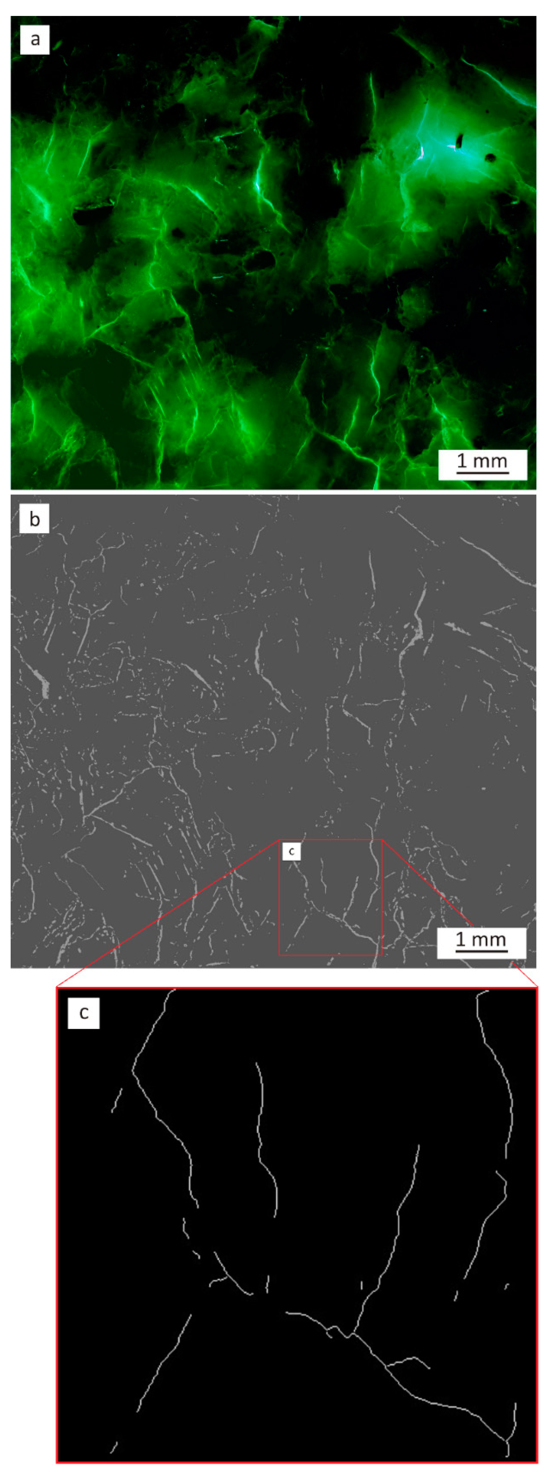
Figure 4.
Examples of: (a) schematic skeletonized image; (b) branch point detection of the intersecting fractures; and (c) division to individual objects. Identification of the end points (marked with yellow) and centre points (marked with orange). Adapted from Kovács et al. [13].
Figure 4.
Examples of: (a) schematic skeletonized image; (b) branch point detection of the intersecting fractures; and (c) division to individual objects. Identification of the end points (marked with yellow) and centre points (marked with orange). Adapted from Kovács et al. [13].
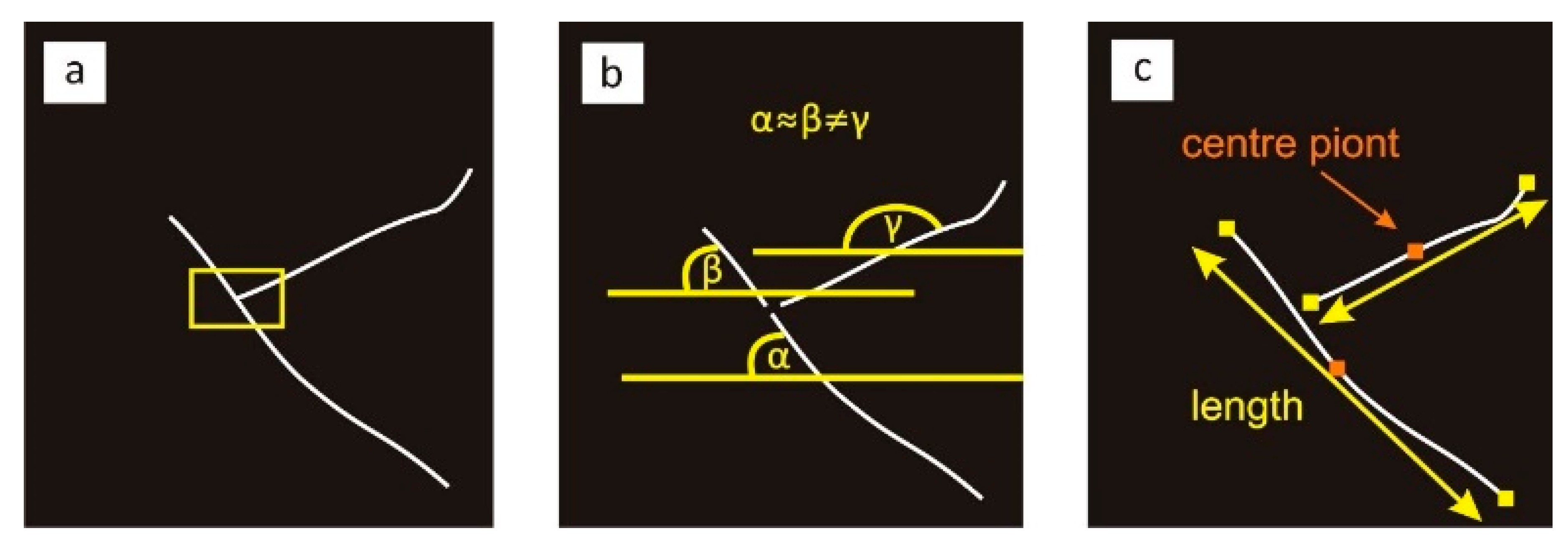
Figure 5.
The microfracture network parameterisation process workflow and steps taken, including the used algorithms. Adapted from Kovács et al. [13].
Figure 5.
The microfracture network parameterisation process workflow and steps taken, including the used algorithms. Adapted from Kovács et al. [13].
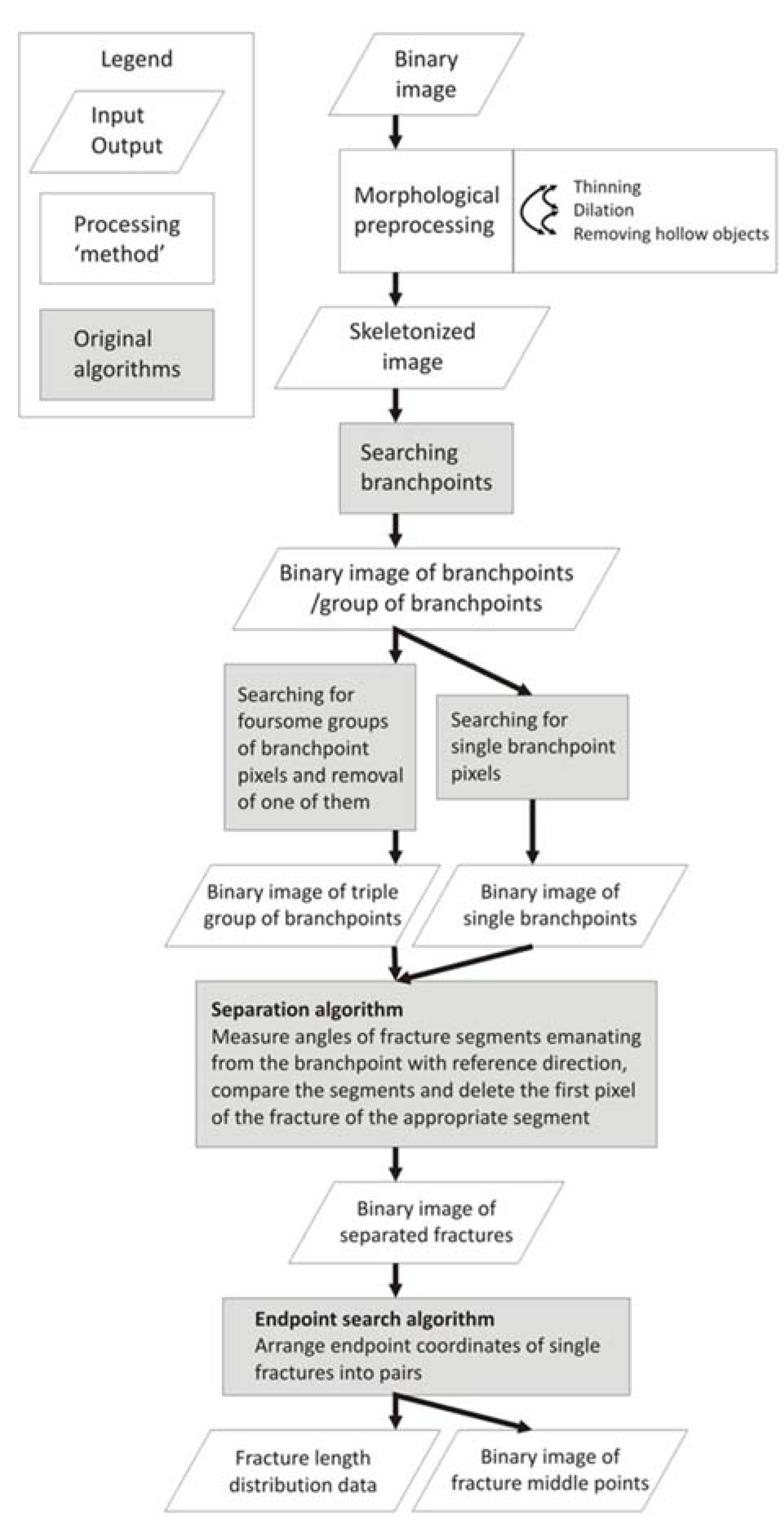
Figure 6.
Schematic image of the models consisting of both pegmatoid granite (PGR) and gneiss (VGN). Volumetric content of PGR increases with 25% increments (a–e). The size of the models is 10 m × 10 m × 10 m.
Figure 6.
Schematic image of the models consisting of both pegmatoid granite (PGR) and gneiss (VGN). Volumetric content of PGR increases with 25% increments (a–e). The size of the models is 10 m × 10 m × 10 m.
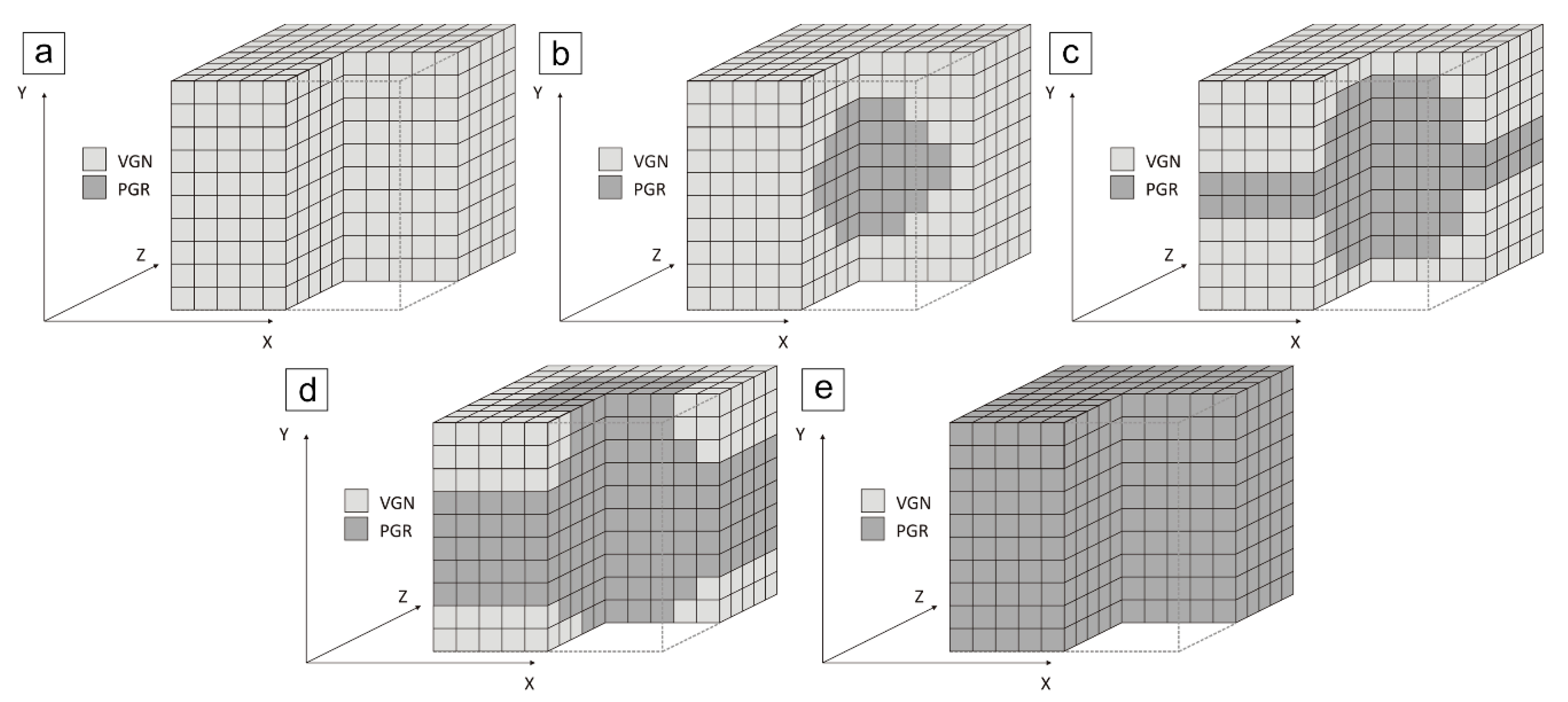
Figure 7.
Example of the visualized results of modelling in a 2-D section of a model with 75% pegmatoid granite and 25% gneiss. Coloured fractures compose connected clusters. Size of the image is 10 m × 10 m.
Figure 7.
Example of the visualized results of modelling in a 2-D section of a model with 75% pegmatoid granite and 25% gneiss. Coloured fractures compose connected clusters. Size of the image is 10 m × 10 m.

Figure 8.
Density vs. the fractal dimension of the fracture midpoints, D. Red is pegmatoid granite, blue is gneiss. Adapted from Kiuru et al. [4].
Figure 8.
Density vs. the fractal dimension of the fracture midpoints, D. Red is pegmatoid granite, blue is gneiss. Adapted from Kiuru et al. [4].
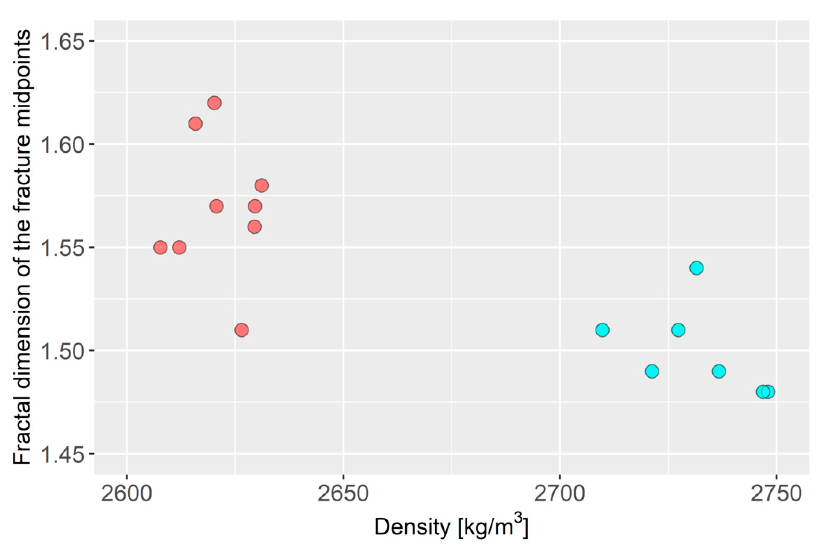
Figure 9.
Example of the resulting fracture networks: (a) gneiss (VGN); (b) pegmatoid granite (PGR). Size of the images is 10 m × 10 m.
Figure 9.
Example of the resulting fracture networks: (a) gneiss (VGN); (b) pegmatoid granite (PGR). Size of the images is 10 m × 10 m.
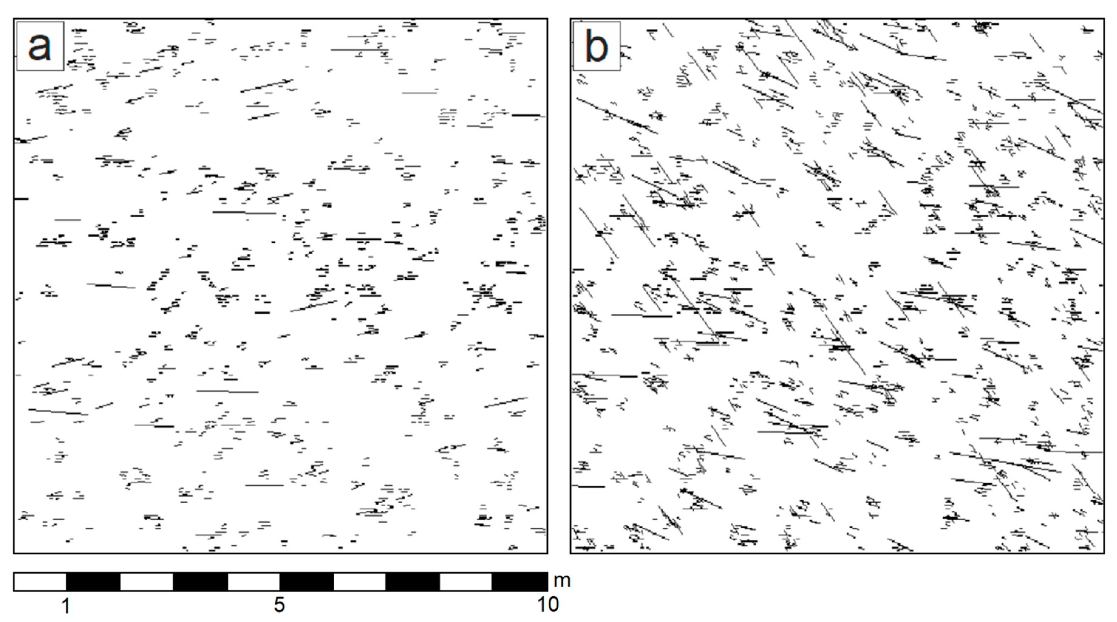
Figure 10.
Results of the discrete fracture network (DFN) simulations. Composition of the models (volumetric content of PGR) are blue = 0%, green = 25%, yellow = 50%, orange = 75%, red = 100%. Remainder of the modelled volume is VGN.
Figure 10.
Results of the discrete fracture network (DFN) simulations. Composition of the models (volumetric content of PGR) are blue = 0%, green = 25%, yellow = 50%, orange = 75%, red = 100%. Remainder of the modelled volume is VGN.
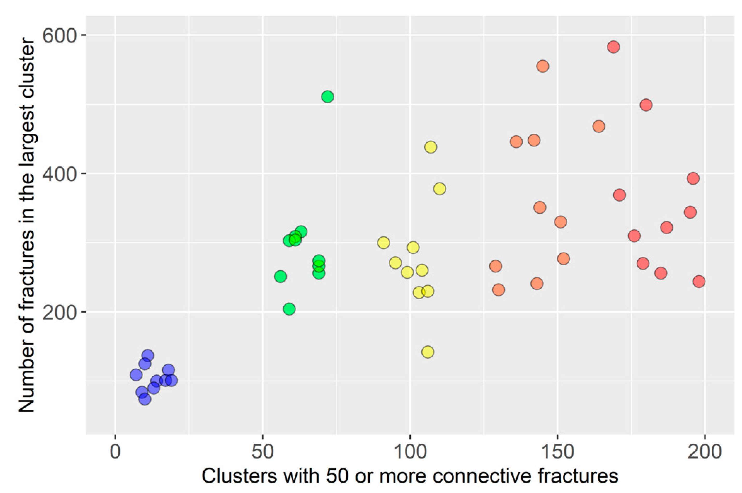
Figure 11.
Fracture length index E* and constant F plotted against physical properties. Red is PGR and light blue is VGN.
Figure 11.
Fracture length index E* and constant F plotted against physical properties. Red is PGR and light blue is VGN.

Table 1.
Descriptive statistics of select tested and calculated properties. Min is the minimum value, Max is the maximum value, Med is the median value, and SD is the standard deviation. For both rock types, the sample size N = 10.
Table 1.
Descriptive statistics of select tested and calculated properties. Min is the minimum value, Max is the maximum value, Med is the median value, and SD is the standard deviation. For both rock types, the sample size N = 10.
| Rock | Min | Max | Med | Mean | SD | |
|---|---|---|---|---|---|---|
| Density [kg/m3] | VGN | 2710 | 2748 | 2734 | 2732 | 14 |
| PGR | 2608 | 2631 | 2622 | 2622 | 7 | |
| Porosity [%] | VGN | 0.27 | 0.70 | 0.43 | 0.48 | 0.13 |
| PGR | 0.37 | 0.75 | 0.44 | 0.47 | 0.11 | |
| Resistivity R0.1 [Ωm] | VGN | 5310 | 19,500 | 10,600 | 11,371 | 4075 |
| PGR | 1810 | 10,500 | 6810 | 6568 | 2773 | |
| Resistivity R10 [Ωm] | VGN | 4870 | 18,300 | 10,300 | 10,605 | 3946 |
| PGR | 1850 | 10,400 | 6750 | 6486 | 2722 | |
| Resistivity R500 [Ωm] | VGN | 4210 | 16,700 | 9685 | 9669 | 3757 |
| PGR | 1800 | 9910 | 6490 | 6235 | 2577 | |
| Relative permittivity [−] | VGN | 5.4 | 7.4 | 6.4 | 6.5 | 0.7 |
| PGR | 5.3 | 6.2 | 5.6 | 5.7 | 0.2 | |
| P-velocity [m/s] | VGN | 5255 | 6088 | 5530 | 5592 | 252 |
| PGR | 5239 | 6060 | 5861 | 5800 | 238 | |
| S-velocity [m/s] | VGN | 2646 | 3687 | 3195 | 3161 | 323 |
| PGR | 3156 | 3434 | 3222 | 3263 | 88 | |
| PS-ratio [−] | VGN | 1.65 | 2.07 | 1.72 | 1.78 | 0.15 |
| PGR | 1.55 | 1.90 | 1.80 | 1.78 | 0.11 | |
| Poisson’s ratio [−] | VGN | 0.21 | 0.35 | 0.24 | 0.26 | 0.05 |
| PGR | 0.14 | 0.31 | 0.28 | 0.26 | 0.05 | |
| Young’s modulus [GPa] | VGN | 51.4 | 90.1 | 69.1 | 69.0 | 11.8 |
| PGR | 66.7 | 73.7 | 70.1 | 70.4 | 2.0 |
Table 2.
Determined fractal dimensions and fracture length distribution parameters of the microfracture networks. Df is the fractal dimension of the fracture network, D is the fractal dimension of the fracture-midpoints, E* is the fracture length index, and F is a constant of the fracture length distribution model. Depth is measured from the excavated surface.
| Specimen | Rock Type | Density [kg/m3] | Porosity [%] | Depth [m] | Df | D | E* | F |
|---|---|---|---|---|---|---|---|---|
| EDZ109 | VGN | 2710 | 0.40 | 0.10 | 1.62 | 1.51 | 2.24 | 18.18 |
| EDZ110 | VGN | 2737 | 0.27 | 0.16 | 1.78 | 1.49 | 2.23 | 18.54 |
| EDZ112 | VGN | 2748 | 0.70 | 0.34 | 1.72 | 1.48 | 1.85 | 16.77 |
| EDZ114 | VGN | 2747 | 0.53 | 0.45 | 1.61 | 1.48 | 2.07 | 16.95 |
| EDZ180 | VGN | 2727 | 0.39 | 0.56 | 1.59 | 1.51 | 2.82 | 21.06 |
| EDZ181 | VGN | 2721 | 0.38 | 0.74 | 1.64 | 1.49 | 2.51 | 20.00 |
| EDZ182 | VGN | 2732 | 0.40 | 0.80 | 1.67 | 1.54 | 1.90 | 15.90 |
| EDZ155 | PGR | 2612 | 0.75 | 0.09 | 1.66 | 1.55 | 2.17 | 16.40 |
| EDZ156 | PGR | 2608 | 0.61 | 0.15 | 1.63 | 1.55 | 1.92 | 15.47 |
| EDZ157 | PGR | 2616 | 0.43 | 0.29 | 1.63 | 1.61 | 1.93 | 15.91 |
| EDZ158 | PGR | 2630 | 0.37 | 0.35 | 1.65 | 1.57 | 2.35 | 18.24 |
| EDZ159 | PGR | 2629 | 0.41 | 0.40 | 1.63 | 1.56 | 1.65 | 14.69 |
| EDZ161 | PGR | 2620 | 0.45 | 0.62 | 1.61 | 1.62 | 2.24 | 17.68 |
| EDZ162 | PGR | 2631 | 0.45 | 0.68 | 1.62 | 1.58 | 2.25 | 17.81 |
| EDZ163 | PGR | 2626 | 0.48 | 0.73 | 1.69 | 1.51 | 1.96 | 16.80 |
| EDZ164 | PGR | 2621 | 0.37 | 0.79 | 1.66 | 1.57 | 1.99 | 16.80 |
Publisher’s Note: MDPI stays neutral with regard to jurisdictional claims in published maps and institutional affiliations. |
© 2021 by the authors. Licensee MDPI, Basel, Switzerland. This article is an open access article distributed under the terms and conditions of the Creative Commons Attribution (CC BY) license (http://creativecommons.org/licenses/by/4.0/).
Share and Cite
MDPI and ACS Style
Kiuru, R.; Király, D.; Dabi, G.; Jacobsson, L. Comparison of DFN Modelled Microfracture Systems with Petrophysical Data in Excavation Damaged Zone. Appl. Sci. 2021, 11, 2899. https://doi.org/10.3390/app11072899
AMA Style
Kiuru R, Király D, Dabi G, Jacobsson L. Comparison of DFN Modelled Microfracture Systems with Petrophysical Data in Excavation Damaged Zone. Applied Sciences. 2021; 11(7):2899. https://doi.org/10.3390/app11072899
Chicago/Turabian StyleKiuru, Risto, Dorka Király, Gergely Dabi, and Lars Jacobsson. 2021. "Comparison of DFN Modelled Microfracture Systems with Petrophysical Data in Excavation Damaged Zone" Applied Sciences 11, no. 7: 2899. https://doi.org/10.3390/app11072899
Note that from the first issue of 2016, this journal uses article numbers instead of page numbers. See further details here.