Article

Particulate Matter Dispersion Modeling in Agricultural Applications: Investigation of a Transient Open Source Solver

1
Department Engineering for Livestock Management, Leibniz Institute for Agricultural Engineering and Bioeconomy (ATB), Max-Eyth-Allee 100, 14469 Potsdam, Germany
2
Chair of Thermal Processing Technology, Montanuniversitaet Leoben, Franz Josef Str. 18, 8700 Leoben, Austria
3
K1-MET GmbH, Stahlstr. 14, 4020 Linz, Austria
4
Chair of Modeling and Simulation, Faculty of Mechanical Engineering and Ship Technology, University of Rostock, Albert-Einstein-Str. 2, 18059 Rostock, Germany
5
Institute of Animal Hygiene and Environmental Health, Department of Veterinary Medicine, Free University Berlin (FUB), Robert-von-Ostertag-Str. 7-13, 14163 Berlin, Germany
*
Author to whom correspondence should be addressed.
Agronomy 2021, 11(11), 2246; https://doi.org/10.3390/agronomy11112246
Submission received: 27 August 2021 / Revised: 6 October 2021 / Accepted: 3 November 2021 / Published: 6 November 2021

Abstract

:
Agriculture is a major emitter of particulate matter (PM), which causes health problems and can act as a carrier of the pathogen material that spreads diseases. The aim of this study was to investigate an open-source solver that simulates the transport and dispersion of PM for typical agricultural applications. We investigated a coupled Eulerian–Lagrangian solver within the open source software package OpenFOAM. The continuous phase was solved using transient large eddy simulations, where four different subgrid-scale turbulence models and an inflow turbulence generator were tested. The discrete phase was simulated using two different Lagrangian solvers. For the validation case of a turbulent flow of a street canyon, the flowfield could be recaptured very well, with errors of around 5% for the non-equilibrium turbulence models (WALE and dynamicKeq) in the main regions. The inflow turbulence generator could create a stable and accurate boundary layer for the mean vertical velocity and vertical profile of the turbulent Reynolds stresses R11. The validation of the Lagrangian solver showed mixed results, with partly good agreements (simulation results within the measurement uncertainty), and partly high deviations of up to 80% for the concentration of particles. The higher deviations were attributed to an insufficient turbulence regime of the used validation case, which was an experimental chamber. For the simulation case of PM dispersion from manure application on a field, the solver could capture the influence of features such as size and density on the dispersion. The investigated solver is especially useful for further investigations into time-dependent processes in the near-source area of PM sources.

1. Introduction

Particulate matter consists of microscopic particles, which are suspended in the earth’s atmosphere. These microscopic particles can enter the human respiratory system or, depending on their size, can even enter the blood stream and cause severe health problems. These are classified as PM1, PM2.5, PM10 based on the particle sizes with all particles less than 1 μm, 2.5 μm and 10 μm, respectively. The effects of particulate matter exposure may result in premature mortality, aggravation of respiratory and cardiovascular diseases, asthma, chronic bronchitis, decreased lung function and various respiratory and cardiovascular health problems [1]. According to the world health organisation, 4.2 million premature deaths each year can be connected to an excessive exposure to PM [2].
Agriculture is one of the main producers of PM and causes approximately 20 % of the global particulate matter emissions [3,4,5], where the largest share is emitted from livestock housing systems, fertilizer application and field cultivation operations [6,7,8]. For  livestock housing systems in Europe, poultry and pig barns are the main contributors of particulate matter emissions from the agricultural sector with 50% and 30%, respectively [9]. Besides the harmful effects of PM, which are only due to it’s size properties, it contains additional potential health hazards when acting as a carrier for pathogens [10,11]. These pathogens can consist of bioactive components such as antibiotics or endotoxins, and microorganisms such as viruses, bacteria, and fungi [12], and spread diseases that are harmful either for other animals or (in case of zoonosis) for human beings. This is especially important in the immediate vicinity of the PM source, where an increased load of these pollutants can be measured [13]. In order to assess the pollution of PM and to investigate potential mitigation strategies to reduce harmful immissions for humans living or working in an environment near to the pollutant sources, the proper modeling of the transport processes of PM in the air can be of great help. For this purpose, the use of computational fluid dynamics (CFD) is an obvious approach.
A common way to simulate the transport of particles in air using CFD is to solve the flowfield of the air as a continuous phase (Eulerian field), and the particles as a discrete phase (Lagrangian field). Here, the flow field of the air is at first simulated using a Reynolds-Averaged Navier–Stokes (RANS) approach in most cases (described, e.g., in [14]). After that, the transport of particles in this flow field is simulated by solving Newton’s equations of motion for each particle, with forces resulting from the flowfield, called the Lagrangian approach. As the RANS approach provides only stationary results, particles would always follow the same stream lines, and the turbulent diffusion of particles cannot be modeled. To account for this, e.g., random walk models can be implemented, which introduce a predefined turbulence on the pathways of the particles [15]. A majority of previous studies for the simulation of PM in an agricultural context follow this approach. For example, Nimmatoori and Kumar [16] investigated the dispersion of PM from field applications with the proprietary solver FLUENT. They studied different RANS turbulence models, and found a significant impact on the particle dispersion characteristics, depending on the choice of turbulence model. Quinn et al. [17] investigated different steady-state approaches to model serial pollutants from agricultural buildings. They found that the inadequate resolution of the flow features is the main reason for the inaccurate results in the near-source region and concluded that further work is needed on non-steady-state simulations for dispersion modeling.
Different advanced turbulent models, with a direct coupling of the discrete phase, were investigated in [18] for indoor applications. They found that, for unsteady-state particle dispersion, large-eddy simulations (LES), coupled with Lagrangian solving of the particle phase, performed the best. The use of transient LES to solve the Euler field has several advantages, compared to steady-state RANS. First, no assumptions have to made regarding the main scales of turbulence (only on the small, isotropic scales), and so the error introduced due to the applied turbulence model is smaller than in RANS (comprehensively discussed in [19]). Second, dynamics such as fast-changing wind directions or wind speeds and their influence on the dispersion of PM are captured by transient LES, which is not possible with the RANS approach, which is steady-state by nature.
Few studies on PM dispersion modeling in an agricultural context can be found that apply transient LES to solve the Euler field. For example, Deetz et al. [20] studied the dispersion of PM10 from a dust event in northeastern Germany by using the numerical model COSMO-ART, which is an extension of the operational weather forecast model COSMO of the German Weather Service (DWD) [21]. Faust et al. [22] couples COSMO with their own Lagrangian particle dispersion model to simulate the PM dispersion of a soil particle plume. However, these studies were done for the transport of PM over large distances (up to several hundreds of kilometers), with grid resolutions typically in the range of 100–1000 m and hence not suitable for the simulation of near-source transmission and immission processes. Also, the discrete phase is simulated with respective turbulence models to take into account turbulent diffusion. Probably due to the high computational costs, little research in the use of transient open source solvers with a direct coupling of the particle phase and the gaseous phase for near-source agricultural applications was done so far. To close this gap, this study aims to investigate the use of an transient open source solver for the simulation of transport processes of PM in the near field of typical agricultural applications. The goal was to (1) validate the velocity field (2) validate the transport of particles, (3) validate a boundary condition for the cost-effective way to generate a turbulent wind field, and (4) demonstrate the validated solver with an example application, namely the the application of manure on a field.
The paper is organized as follows. Section 2 gives an overview on the theory of large eddy simulations and particle transport. Section 3 describes the validation process of the solver and presents the results from the validation (goals 1 and 2). Section 4 describes the application of the solver for the manure application and presents the simulated results (goals 3 and 4). Section 5 discusses these results and Section 6 presents the drawn conclusions. The workflow of this study is briefly illustrated in Figure 1.

2. Materials and Methods

The following section provides a brief overview about the solving techniques for the (continuous) flow field and the (dispersed) particle phase. Two different turbulence modelling approaches, namely, RANS and LES, were applied to calculate the turbulent flow fields. Based on these flow fields, the transport of the particulate matter is predicted by two different Eulerian–Langrangian solvers implemented in the open source CFD-framework OpenFOAM. Moreover, the complete numerical setup (e.g., computational domain, boundary conditions, solver setups) and mesh convergence study, as well as the validation of the numerical results, will be discussed in the following. To provide a good reproducibility, all OpenFOAM-related terms and specific settings will be shown in typewriter font.

2.1. Solving the Flow Field Phase

Large Eddy Simulations is a method of turbulence modelling focusing on the behaviour of large eddies by spatially filtering the transient Navier–Stokes equations. LES reduces the computational cost by ignoring the eddies with smallest length scales. In LES, the vortices are subdivided into large resolved vortices, which transport most of the energy in the flow, and small subgrid-scale (SGS) vortices, which are modeled with an SGS turbulence model. The separation of these large and small vortices is done using spatial filtering. Filtering the Navier–Stokes equations results in Equation (1), where τ i j S G S = u i u j ˜ u ˜ i u ˜ j is the SGS stress, which considers the effect of small vortices.
ρ u ˜ i t + ρ u ˜ i u ˜ j x j = ρ x j ν u ˜ i x j τ i j S G S p ˜ x i + ρ g i
These stresses are calculated using SGS turbulence models. One of the most popular SGS turbulence models is the Smagorinsky model [23]. This uses the idea of Prandtl mixing theory and calculates the SGS stress as
τ i j S G S 2 ν S G S S ˜ i j + 1 3 τ k k S G S
According to Smagorinsky, the subgrid viscosity is calculated as
ν S G S = ( C s Δ ) 2 2 S ˜ i j S ˜ i j , S ˜ i j = 1 2 u ˜ i x j + u ˜ j x i
where S ˜ i j is the strain rate tensor and C s is the constant of Smagorinsky. The constant of Smagorinsky was theoretically estimated in the range of 0.17–0.21. The Smagorinsky model is a zero-equation model and is based on the local equilibrium assumption. Even though the model is simple and stable, laminar flow is not modelled, damping is necessary for near wall regions and the Smagorinsky constant is problem-dependent.
To improve the simulation results for wall-bounded flows, the Wall-adapting Local Eddy viscosity (WALE) model was proposed considering the square of the velocity gradient tensor as
ν S G S = C w Δ 2 S i j d S i j d 3 / 2 S ˜ i j S ˜ i j 5 / 2 + S i j d S i j d 5 / 4
where C w is the model constant in the range of 0.55 C w 0.60, which is appropriate for C s = 0.18, and S i j d is the traceless symmetric part of the square of the velocity gradient tensor [24]. The WALE model is able to handle transition and damping is not necessary for the near-wall region.
Smagorinsky, and WALE are zero equation models, whereas the model proposed by Yoshizawa and Horiuti is the one-equation eddy viscosity model, which additionally solves a transport equation to compute subgrid kinetic energy k S G S . According to this model, the subgrid scale viscosity is computed as
ν S G S = C k Δ k S G S , k S G S = 1 2 ( u i 2 ¯ u ¯ i 2 )
in terms of the subgrid kinetic energy [25,26]. Similar to the Dynamic Smagorinsky model, a dynamic one equation eddy viscosity model was proposed by using a dynamic procedure to calculate the coefficients. In these one-equation models, no assumption was made of local equilibrium between the subgrid-scale energy production and dissipation rate. These one-equation models tend to produce more accurate results than the zero-equation models [27].
The used software Package OpenFOAM contains a library with a broad range of SGS scale turbulence models. For this study, we investigated the models of Smagorinsky, TKE, dynamic TKE, and the wall-adapting local eddy viscosity (Smagorinsky, oneEqTKE, dynTKE and WALE, respectively).
Another way to solve the flow field is the Reynolds Averaged Navier Stokes (RANS) equations approach. With the RANS equations, only the mean flow is solved, while all turbulence scales are parametrized. For the turbulence parametrization, a turbulence model is applied. A comprehensive overview of the turbulence models within the RANS approach is given in [14].

2.2. Solving the Particle Phase

Particle modelling in CFD is considered as multiphase approach since the particles in the fluid becomes a separate phase. In CFD, the multiphase modelling can be done either by Euler-Euler or Euler-Lagrange approach. In the Euler-Euler approach, the particles are considered as a continuous phase whereas in the Euler-Lagrange approach, the particles are considered as a discrete phase and Newton’s equations for motion are solved for the particle phase to track the trajectories of the particle. The Euler-Euler approach is suitable for large particles, where the particle size is greater than the cell-size of the mesh. The Euler-Lagrange approach is suitable for smaller particles [28].
As mentioned above, in the Lagrangian framework, the motion of the particles is calculated by solving a set of ordinary differential equations along the particle trajectories. According to Newton’s second law of motion, this requires the consideration of all relevant forces acting on the particle, e.g., drag force, gravitational and buoyancy force or pressure gradient force. Since analytical solutions for the majority of the particle forces are only available for small particle Reynolds numbers (i.e., Stokes regime), the determination of the considered particle forces is based on different empirical correlations derived from experiments. In most particle-laden flows, the drag force dominates for the particle motion [29] and is expressed in terms of a drag coefficient C D , which allows for the calculation of the drag force not only for small-particle Reynolds numbers ( Re p < 0.5 ), where viscous effects dominate and no separation is observed, but also for the transition region (i.e., 0.5 < Re p < 1000) and fully turbulent region or Newton regime (above Re p 1000 ). The applied drag models are based on the particle Reynolds number, which is defined as:
Re p = ρ f D p | u f , i u p , i | μ f ,
with the velocity u f , i , density ρ f and the dynamic viscosity μ f of the fluid (or continuous phase), the particle diameter D p and particle velocity u p , i , as well as the magnitude of the relative slip velocity | u f , i u p , i | . Assuming rigid and sparsely distributed spherical particles (i.e., dilute dispersion), the drag coefficient is determined using the drag model proposed by Putnam [30]:
C D = 24 Re p 1 + 1 6 Re p 2 / 3 if Re p 1000 0.424 if Re p > 1000 ,
which is suitable for high particle Reynolds numbers ( Re p 1000 ) and ensures the correct limiting behavior within the Newton regime ( Re p > 1000 ) . Based on the calculated drag coefficient, the general equation of particle motion is used to evaluate the corresponding drag coefficient for spherical particles as follows:
F D , i = C D π D p 2 8 ρ f ( u f , i u p , i ) | u f , i u p , i | .
Besides the Putnam drag model, various other drag models exist to account for non-spherical particles or different fluid/particle volume fractions. A widely used drag model for higher particle volume fractions ϕ p (i.e., dense dispersed two-phase flows), which is usually the case in fluidization, is the Ergun–Wen–Yu model. This combines the well-known Ergun equation (see, e.g., [29,31]) for fluid flows in packed beds and the drag model for spherical particles proposed by Wen and Yu [32]. Thus, for fluid volume fractions ϕ f smaller than 0.8 , the particle drag force is directly calculated from the Ergun equation, whereas, for higher fluid volume fractions (i.e., ϕ f 0.8 ), the drag coefficient can be estimated by the Wen–Yu model [31,32]:
C D = 24 Re p 1 + 0.15 Re p 0.687 ϕ f 2.65 if Re p 1000 0.44 ϕ f 2.65 if Re p > 1000 ,
which is the drag coefficient formulation originally proposed by Schiller and Naumann [29], but accounting for the fluid volume fraction ϕ f . Analogously to the application of Putnam’s correlation, Equation (7), the estimated drag coefficient is then used to calculate the particle drag force from the general equation of particle motion, Equation (8).
One of the most important parameters to characterize fluid–particle flows is the Stokes number St = τ p / τ f , which relates the particle response time τ p to the characteristic time of the flow field τ f . If the Stokes number is less than <0.1, the particles follow the flow instantaneously [33], and as the Stokes number increases, the particles start to deviate from the flow. In particle modeling, it is also important to consider the phase coupling to decide how the particles interact with each other and the fluid. Elgobashi [34] classified particle-laden turbulent flows based on the volume fraction of particles ϕ p . For values of ϕ p 10 6 the particles follow a one-way coupling where the momentum transfer from particles to the flow is negligible. For values of 10 6 < ϕ p 10 3 , the momentum transfer is large and affects the flow, which is termed a two-way coupling. In this region, when the particle response time τ p decreases, the dissipation rate increases, whereas an increase in τ p increases the production of turbulence energy. When ϕ p > 10 3 , the flow is dense and particle–particle collisions occur, along with a momentum transfer between the particles and fluid, which is termed a four-way coupling.

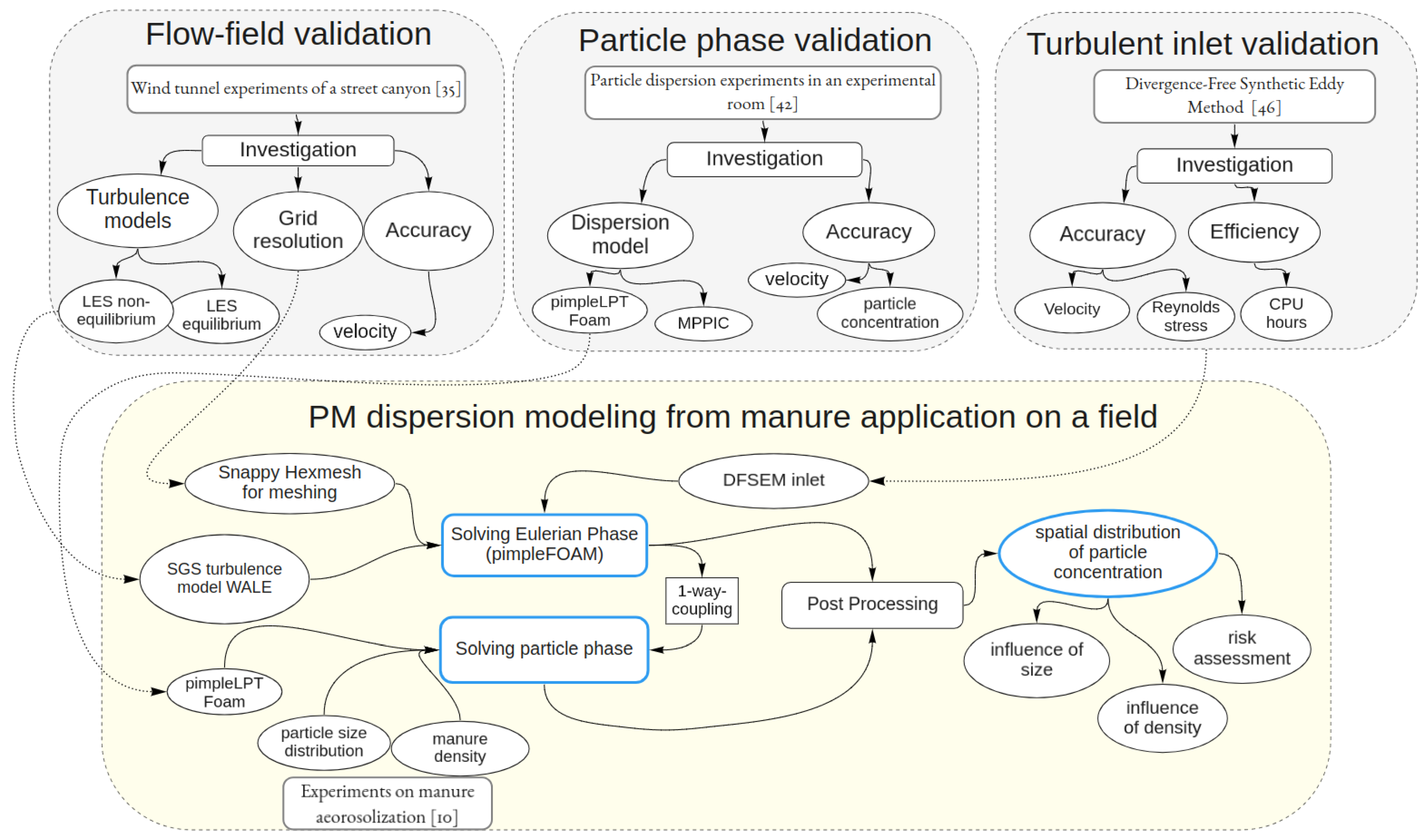
3. Validation of the Solver

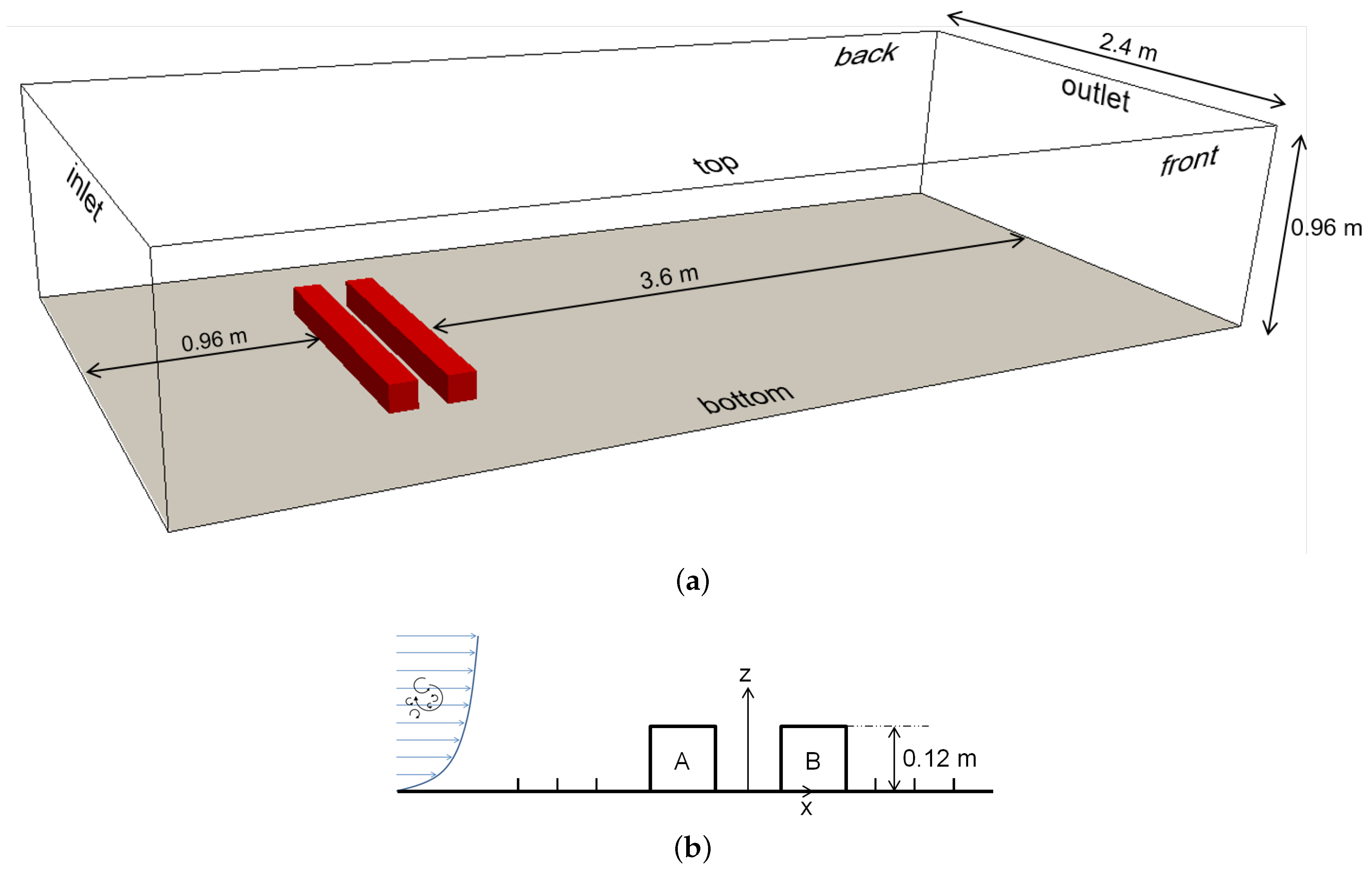
3.1. Validation of the Flow Solver

To validate the flow solver, an urban street canyon study in an atmospheric boundary layer wind tunnel by [35] was used. This study was chosen because it provided very detailed information on the flowfield in a fully turbulent environment with near obstacles, which is similar to a large number of applications for near field particle modeling in agricultural applications. Wind tunnel experiments were carried out in a test section of width 2 m, height 1 m and length 2 m, with a boundary layer flow with mean velocity profile exponent α = 0.30. A 1:150 scaled model of two buildings was introduced in the test section with dimensions in the natural scale of length L = 180 m, width W = 18 m and height H = 18 m, forming a street canyon. Flow measurements were performed using Lased Doppler Anemometry (LDA).

3.1.1. Geometry

The modeled buildings have the dimension of height H = 0.12 m along the z axis and Length L = 1.2 m along y axis after scaling. The distance between the buildings is 0.12 m.
The domain has an upstream length of 8H and downstream length of 30 H, with a domain height 8 H. The domain width along the y axis is 20 H. The origin of the domain lies in the bottom wall in the mid-plane and in between the centre of the street canyon, as shown in Figure 2. The flow is along the positive x-direction.

3.1.2. Meshing

Three different meshes were generated, all consisting of purely hexahedral cells with the OpenFOAM integrated mesh generators blockMesh and snappyHexMesh. At first, the domain was meshed with more cells near the bottom wall by grading the cells along the height of the domain. The domain was meshed with 260 × 92 × 70 (coarse), 313 × 110 × 70 (medium) and 375 × 130 × 85 cells (fine). Mesh refinement was performed around the buildings and the canyon formed by the buildings. A single-refinement region was created for the coarse mesh and the mesh was refined two times for medium and fine meshes.
The meshes consisted of 2,103,476 computational cells for the coarse mesh, 5,038,022 cells for the medium mesh and 10,559,532 cells for the fine mesh. The  y + values for the meshes are described in Table 1. Even with the finest mesh and inflation layers at the walls, a y + < 1 could not be achieved in all regions; hence, a wall function using Spalding’s law of the wall was applied, which is known to perform well in all regions of y + [36,37].

3.1.3. Boundary Conditions

The inlet boundary conditions were chosen as suggested by C. Gromke et al. [35]. The inlet velocity profile follows the power law approach as in Equation (10) with mean velocity profile exponent α = 0.30 and flow velocity of U( z r e f = H) = 4.7 m/s and turbulent kinetic energy follows the profile in Equation (11) with boundary layer depth δ , friction velocity u τ = 0.52 m/s and Cμ = 0.09.
U ( z ) U ( z r e f ) = z z r e f α
k = u τ C μ 1 z δ
The pressure at the inlet was defined with a Dirichlet boundary condition (zeroGradient). At the outlet, the boundary condition for velocity was set to zeroGradient and the pressure to fixedValue. The top, front and back boundaries are set as symmetryPlane, meaning a free-slip condition. The boundaries’ bottom and buildings are considered walls, where the velocity is set to zero.

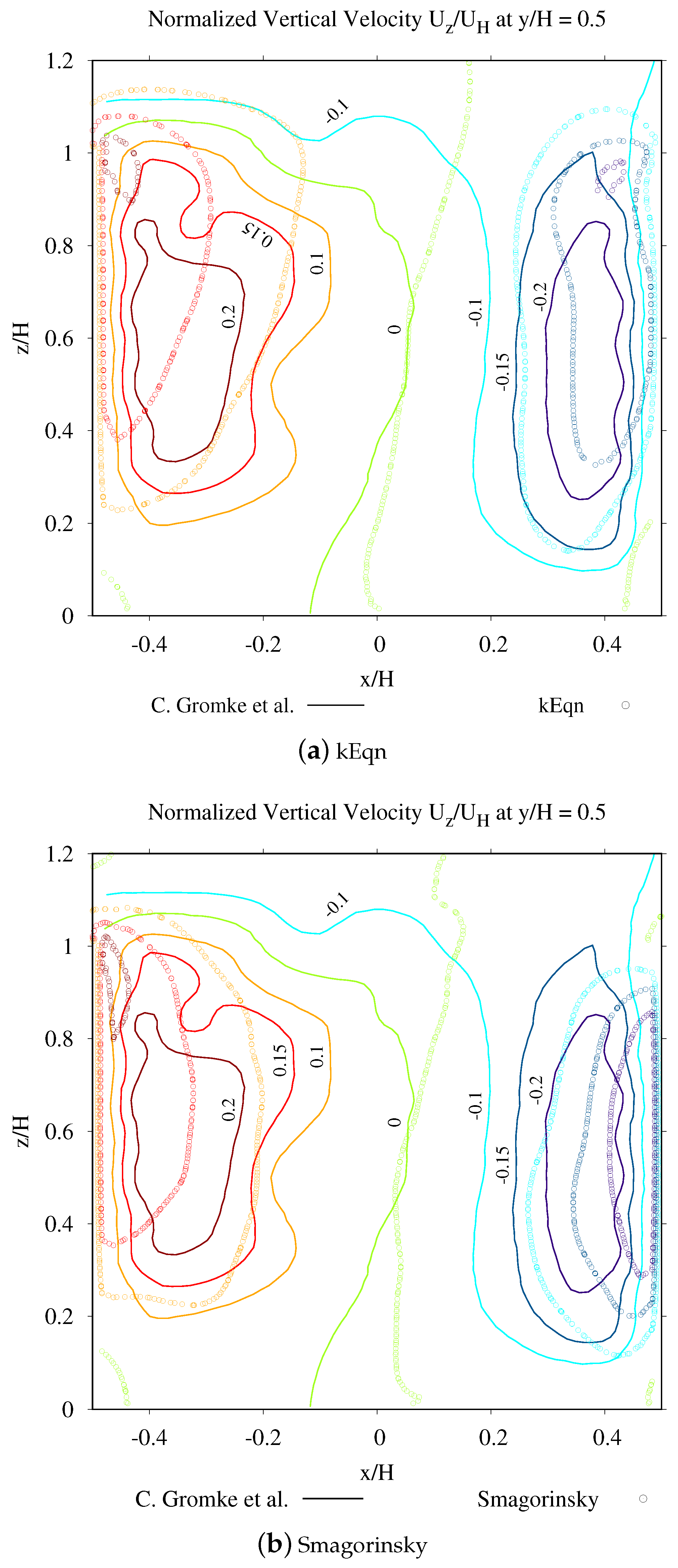
3.1.4. Solver Setup and Turbulence Modeling

Incompressible Large Eddy simulations were set up using the pimpleFoam solver, which is a combination of the Pressure-Implicit with Splitting of Operators, [38] (PISO) solver and the Semi-Implicit Method for Pressure Linked Equations (SIMPLE) algorithm, [39]. It has the advantage of a fast convergence for transient simulations, as described, e.g., by [40]. An adaptive time stepping was chosen with a Courant number no higher than 1.
The spatial discretization was performed using second-order linearUpwind schemes, and the time variable was discretized with the second-order backward scheme, which are both described in [41].
In this study, the influence of four different subgrid scale turbulence models on the flow field were investigated, namely kEqn, dynamicKEqn, WALE, and Smagorinsky, all described in Section 2.1.
The simulation was carried out for 5 s with the help of 24 processors running for 6 days. Considering the flow velocity at the height H, UH = 4.7 m/s, the flow passes through the entire domain five times in 5 s and, in the region of interest, near the buildings, the flow passes through approximately 40 times. Hence, a period of 5 s was considered sufficient for the entire simulation.

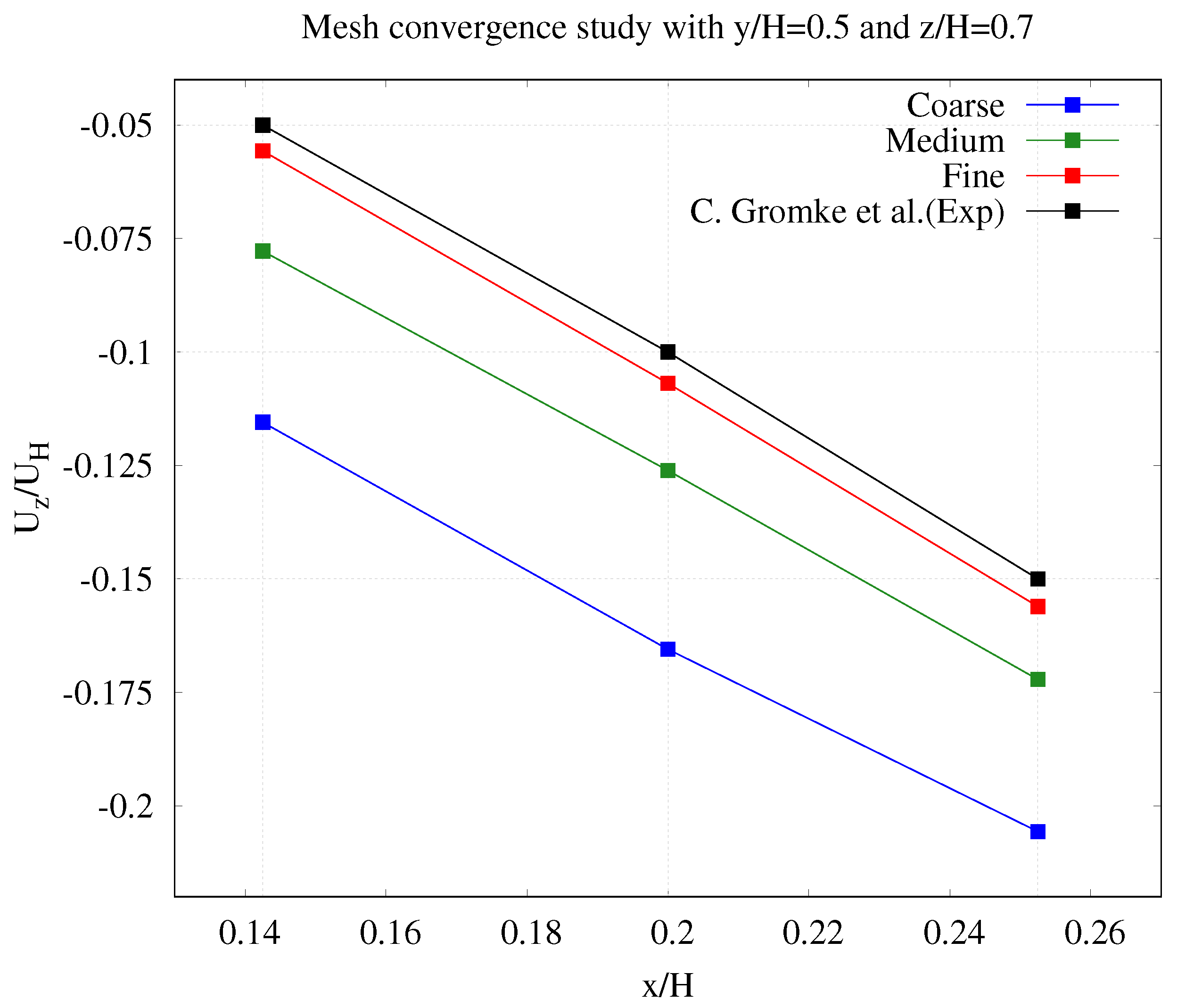
3.1.5. Mesh Convergence

Mesh convergence study was carried out using the dynamicKEqn turbulence model and the experimental results [35] at three different points in the street canyon along a horizontal line on the xz-plane at y = 0 (symmetry plane) and a height of z = 0.7 H. The points are chosen from the experimental results where the normalized vertical velocities Uz/UH are −0.05, −0.1 and −0.15. Hence, the normalized vertical velocities are measured from the simulations at x/H = 0.1425, 0.2 and 0.2525 and compared with the experimental results, as in Figure 3. From the figure, the large influence of the grid size can clearly be seen. At x/H = 0.2525, the relative errors for coarse, medium and fine meshes are 37%, 15% and 4%, respectively. Hence, for all the following simulations, the fine mesh was chosen.

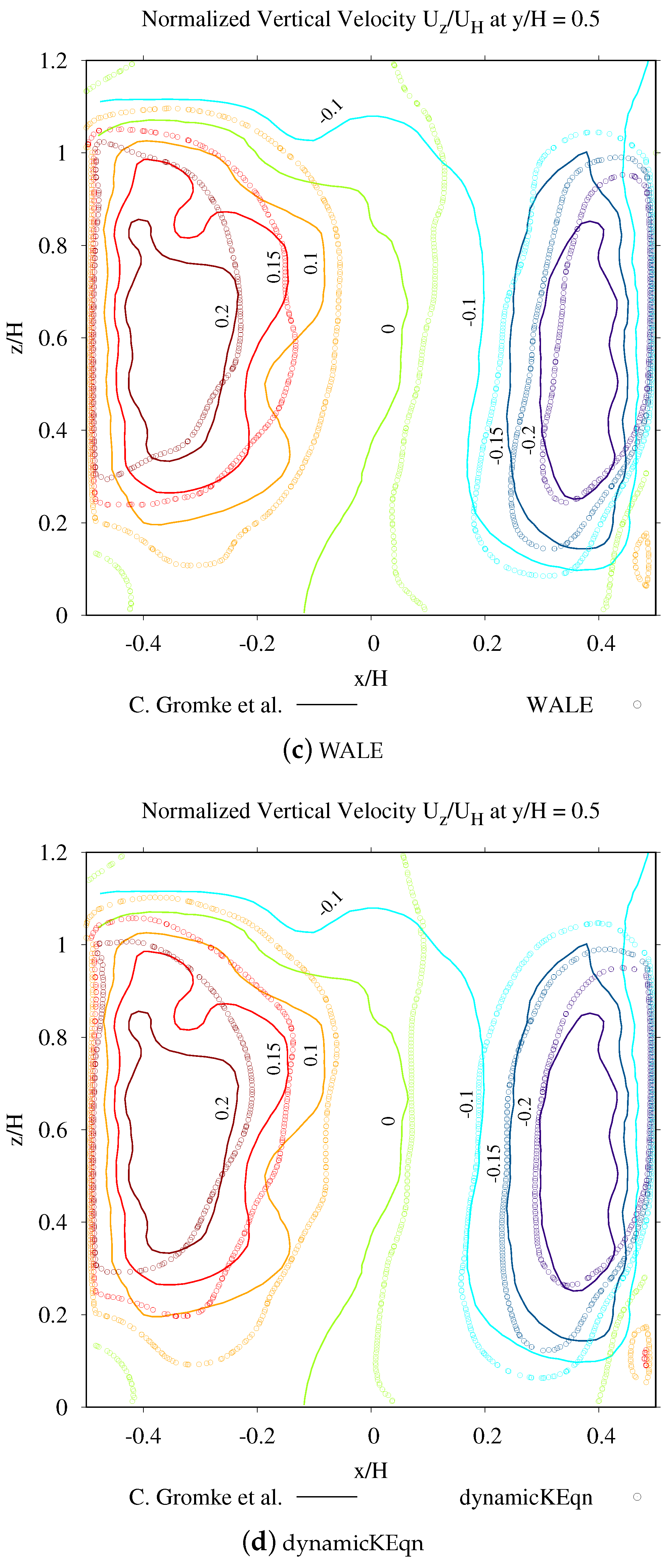
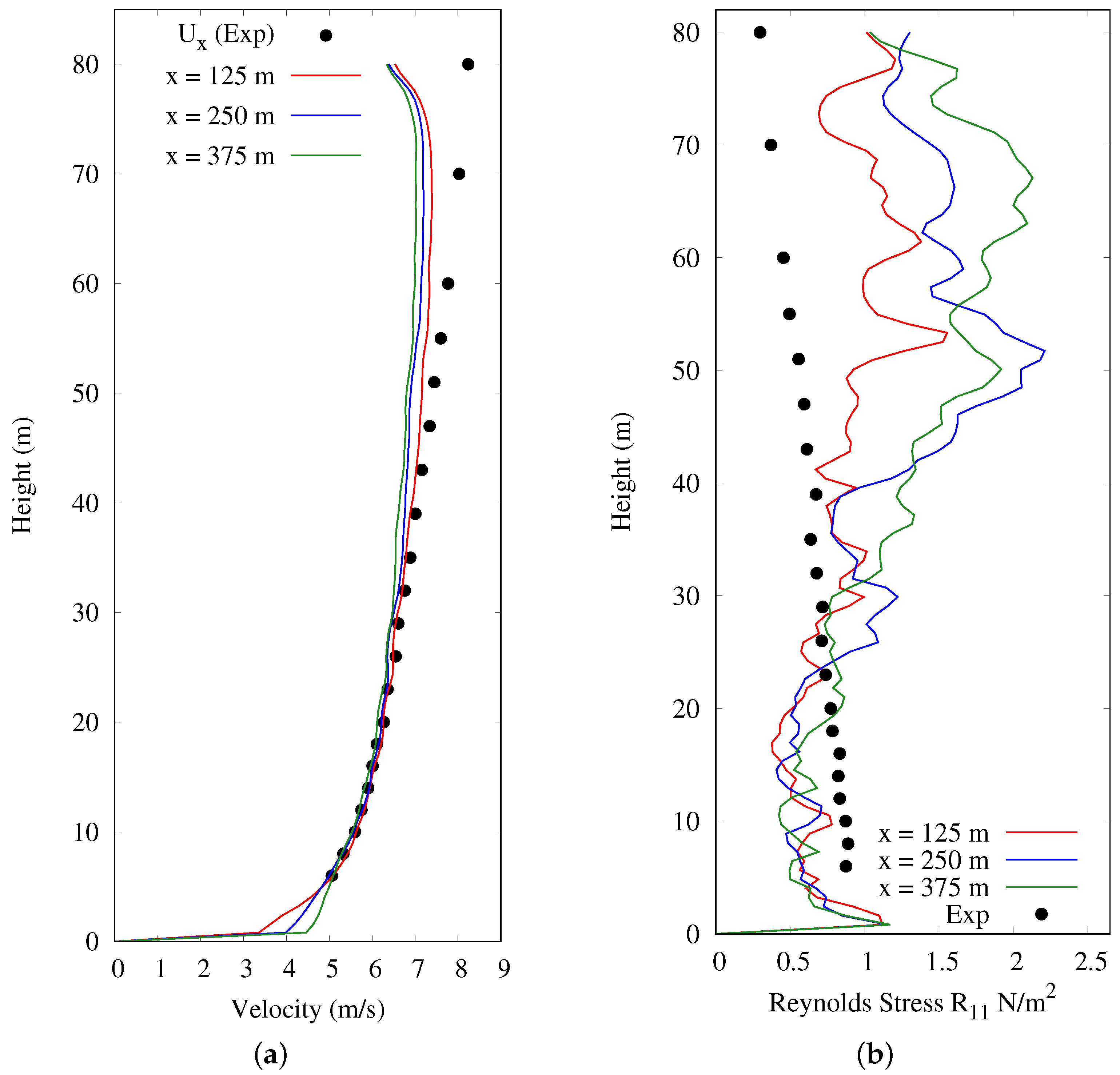
3.1.6. Validation Results of the Flowfield

Figure 4 shows the flowfields simulated with the four different SGS turbulence models. The normalized vertical velocity is shown in isotachs in the XZ-area between building A and building B at y/H = 0.5 and compared with the experimental values. All four SGS models predicted the general pattern of a clockwise vortex formed in the canyon, with negative vertical velocities on the side of building B and positive velocities at building A. A clear difference can be seen between the equilibrium-assumption SGS models kEqn and Smagorinsky in Figure 4a,b and the non-equilibrium SGS models dynkEqn and WALE in Figure 4c,d. Both equilibrium models failed to predict the spatial distribution of velocity contours accurately, especially for the positive-velocity region near building A. Here, both models predicted the velocitiy maxima near the edges of the building whereas, in the experiment, the velocitiy maxima were high near the middle region of the building. On the other hand, the non-equilibrium models WALE and dynamicKEqn performed very well when reproducing the experimental results. On the side of building B, a very good agreement can be seen for the negative velocities towards the middle region, with no noticeable difference between experimental and simulation results for dynamicKEqn. However, near the wall region, all SGS models showed larger deviations from the experimental data. The highest deviations can be seen at the height of z/H = 0.6; the relative error was, depending on the compared velocity contour, in the range of 5–20%. Possible reasons for this are discussed in Section 5.1.

3.2. Validation of the Particle Transport

For the validation of the particle transport solver, high-resolution measurements of particulate matter concentrations (in both time and space) in a fully turbulent flow under well-documented experimental conditions would ideally be found. Unfortunately, these data cannot be found in the literature. As a compromise, the study of [42] was chosen as a reference case to validate against. [42] conducted experiments inside a model room of size 0.8 m × 0.4 m × 0.4 m; see Figure 5. Silver-coated hollow glass spheres of density 1400 kg/m3, with a mean diameter of 10 μm and nominal diameter range between 2 and 20 μm, were injected for a time period of 1800 s. Air-flow velocity and particle concentration were measured using Phase Doppler Anemometry (PDA). The particle concentration was measured at 27 different locations in the mid-plane of the model room along three different x positions.

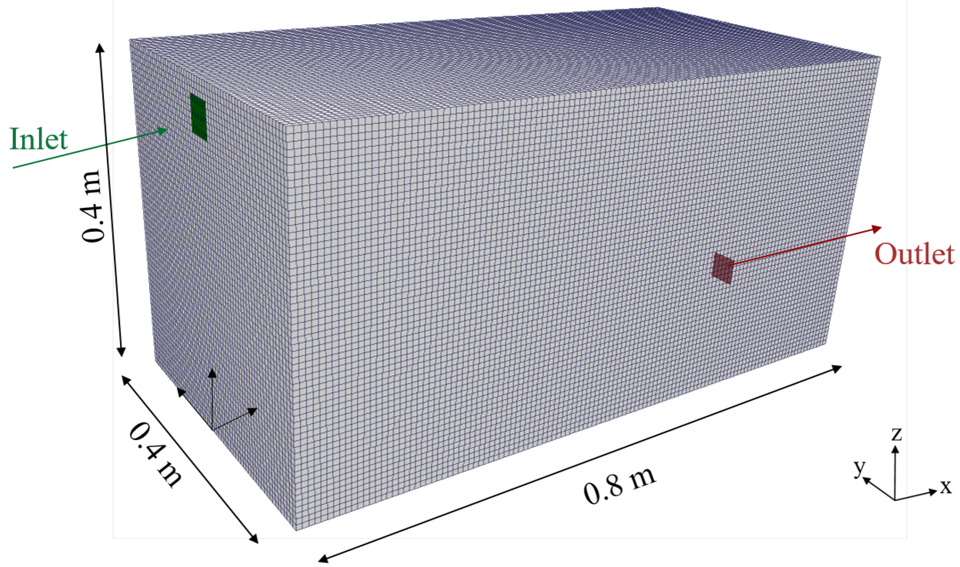
3.2.1. Computational Domain and Meshing

The room was modeled and meshed, as sketched in in Figure 5. The centres of inlet and outlet were located at x = 0 m, y = 0.2 m, z = 0.36 m and x = 0.8 m, y = 0.2 m and z = 0.04 m, respectively, with the same area of 0.04 m × 0.04 m. Two different meshes were created with 221,184 (96 × 48 × 48) and 432,000 (120 × 60 × 60) hexahedral cells. Excepting the inlet and outlet, all other boundaries were considered as walls with a no-slip boundary condition. In both meshes, the  y + was less than 1 in almost all regions except the corners, where maximum values of 6 were reached.

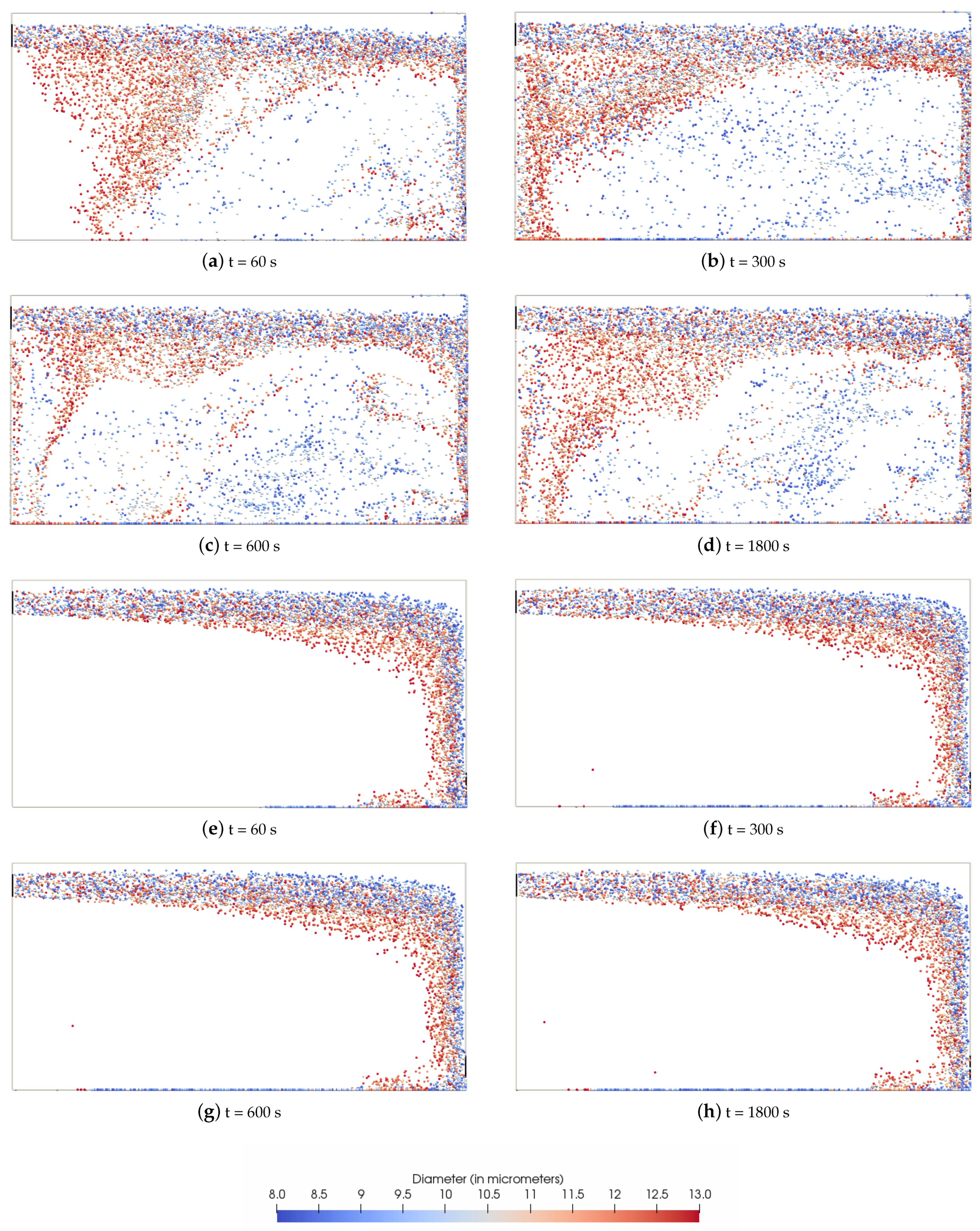
3.2.2. Particle Injection and Simulation

At the inlet, a uniform velocity was set according to the experimental inlet velocity of 0.225 m/s. The particles were injected from the inlet patch for 1800 s. Every second, 1000 particles were injected. To vary the diameter of the particles according to the experiment, a normal distribution model was used, with an expectation of 10 μm. The particle diameters ranged from 8 μm to 13 μm. The density of the particles was set to 1400 kg/m3. The particles were simulated with Gravity, Drag and Pressure forces. Boundary interactions were set to an escape condition when particles reach the outlet, or rebound condition when particles reached the walls.
For the simulation of the particle phase, the influence of different LES and URANS models on the particle concentration was investigated, as well as the influence of two different lagrangian solvers, namely pimpleLPTFoam, in combination with the drag model of Putnam (sphereDrag) and MPPICFoam using the Ergun–Wen–Yu drag model (ErgunWenYuDrag). The multi-phase particle in Cell method [43] is similar to the Discrete Parcel Method (DPM). In DPM, the particle interactions are directly resolved, whereas in MPPIC, particle–particle interactions are represented by models, which utilise the mean values calculated on the Eulerian mesh. pimpleLPTFoam was originally introduced by the Chair of Modeling and Simulation (LeMoS) at the University of Rostock [44,45] for dilute particle-laden flows by combining a DPM-based particle-tracking approach, including four-way phase-coupling capabilities, with the standard OpenFOAM solver pimpleFoam.
Ithen case of URANS, the converged RANS solution was mapped onto the fine mesh and then the particle phase was simulated with pimpleLPTFoam using the kEpsilon model for 1850 s. The particles were injected from 20 s until 1820 s. In the case of LES, the dynamicKEqn turbulence model was used, since it produced better results in the flow-field validation case, as shown in Section 3.1.6.
Both pimpleLPTFoam and MPPICFoam were set up with backward time schemes; a second-order linear scheme for div(phi,U) term and linearUpwind for div(phi,k) term were used. The simulation was carried out for 1850 s with 24 processors, with an average simulation time of 40 h for LES.

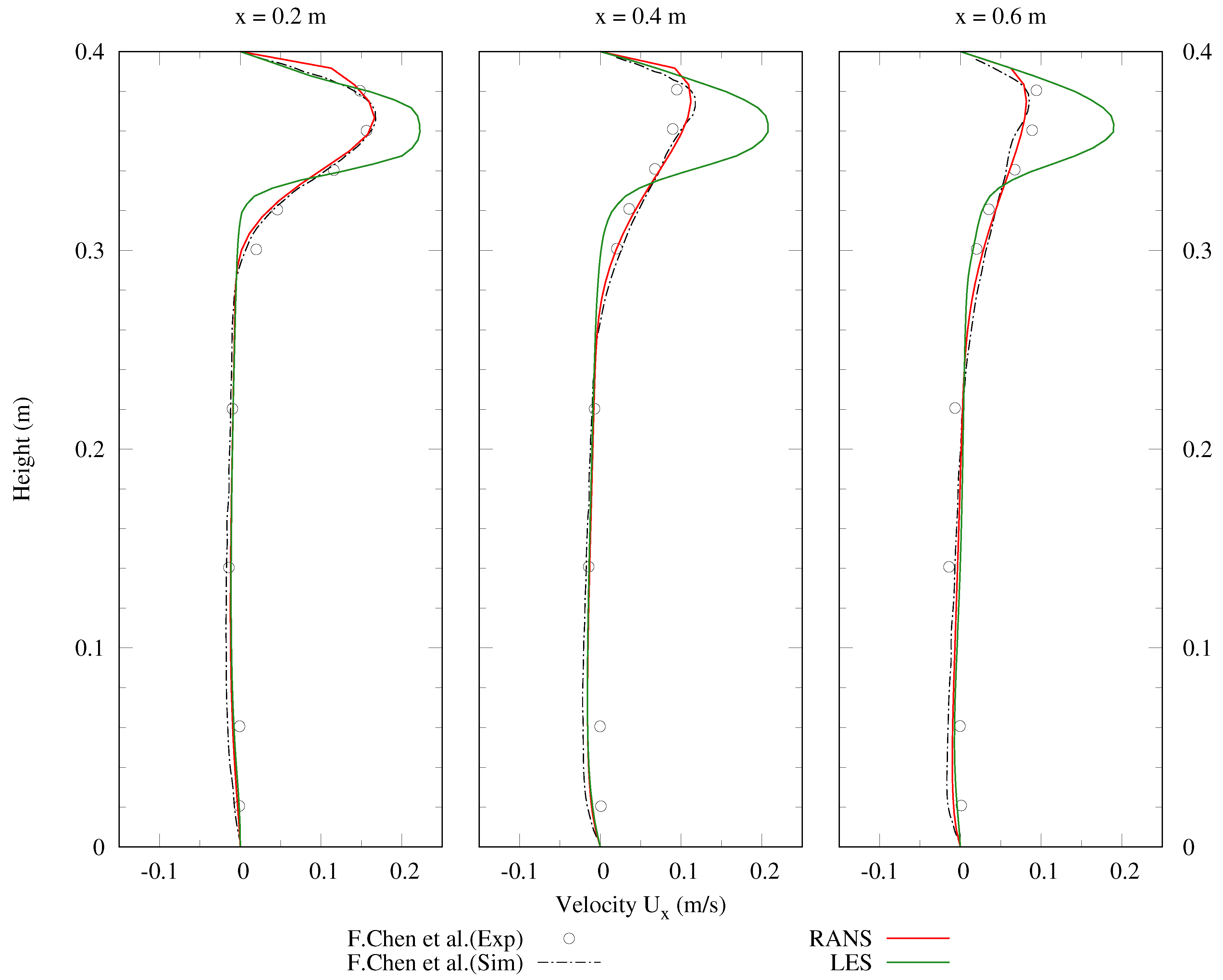
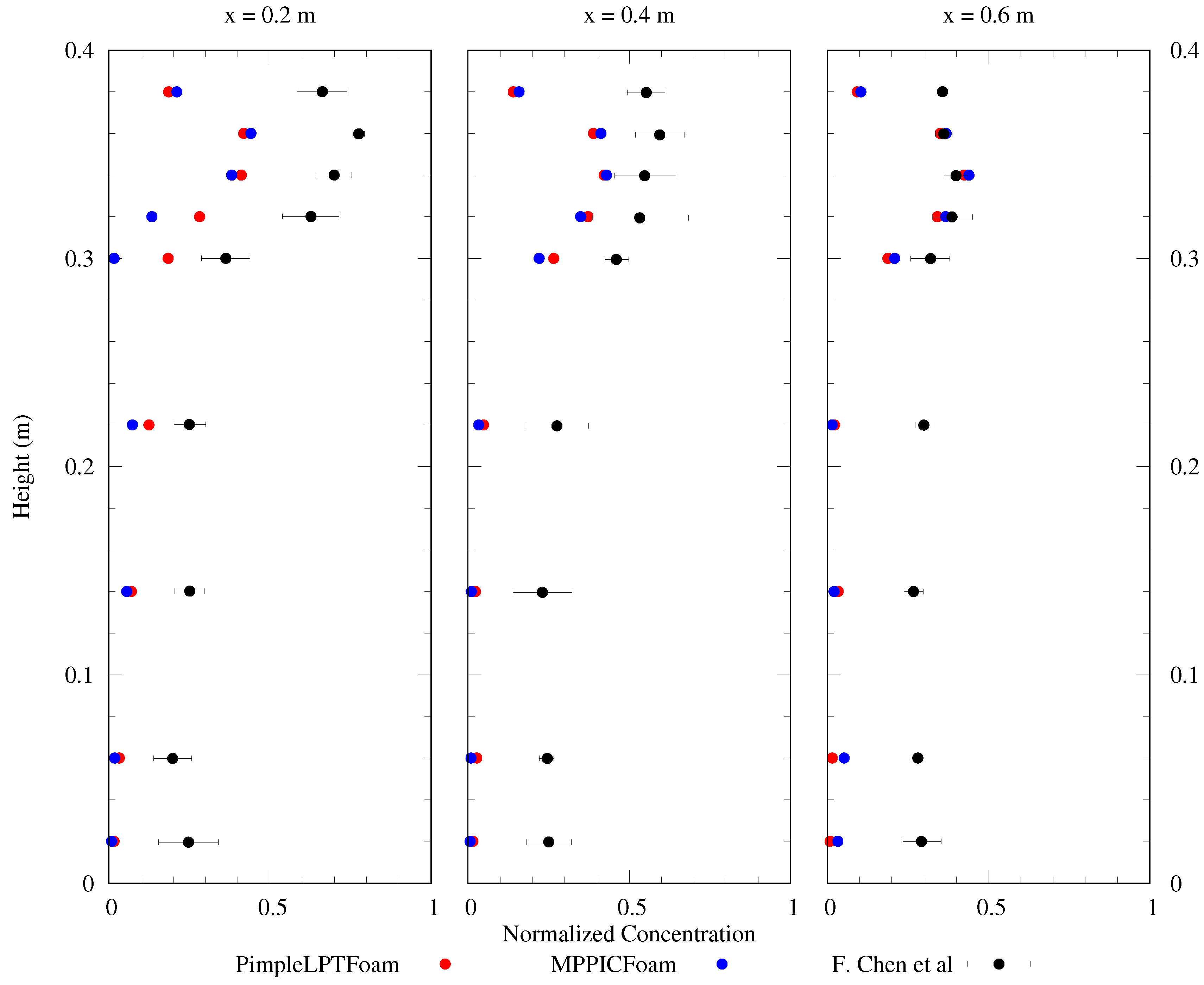
3.2.3. Validation Results of the Particle Transport

The velocity profile Ux from the experiment is compared to the RANS and LES simulations along three lines at x = 0.2, 0.4 and 0.6 m in the mid-plane in Figure 6. The velocity profile from the RANS simulation with the kEpsilon turbulence model predicted the experimental velocity profile very precisely along all three lines. For LES simulation, the velocity profile was time-averaged and then compared. Even though the LES simulation began from the converged solution of the RANS simulation, the velocity along the inlet tends to increase further than the expected experimental values. LES was able to perform well near the wall region and in the region below the inlet, but the velocity values are overpredicted along the inlet. The possible reasons for this are discussed in Section 5.2.
The particle distributions in the domain at four different times are shown in Figure 7. For the LES, the particles are thrown towards the wall near the outlet and hit the wall. Particles with a large diameter tend to fall down due to gravity soon after entering the domain, and then, due to the negative-velocity region below the inlet, they move back, as observed in the experiments. A mixing of particles over the whole volume is generally visible, with slightly higher concentrations below the inlet, along the inlet jet, and at the outlet positioned wall. In contrast, for the URANS, the particles always follow the same path as the flow field and no dispersion is visible in the volume of the domain. Even though the particles with a larger diameter tend to fall earlier within the jet, they only start to fall near the outlet wall. This very uneven distribution can be explained by solving the flow field, which converged after the initial RANS. Due to the lack of turbulence, further simulations with URANS result in stagnation of the flow field, meaning that the particle trajectory at 60 s is the same as the particle trajectory at 300, 600, 1800 s and throughout the simulation.
The time-averaged particle number concentrations of the LES simulations are compared with the experimental results from [42] in Figure 8. For all three vertical sampling lines, the same trend from the experiment with high particle concentrations in the upper third of the domain, and decreasing concentrations towards the floor, is recaptured by the simulations. Both solvers, PimpleLPTFoam and MPPICFoam, show nearly identical results, with the exception of two measurement points at sampling line x = 0.2 m on height 0.3 m and 0.32 m. For all three sampling lines, the simulations underestimated the particle concentrations in the lower two thirds of the domain, with relative errors in the range between −37% (x = 0.2 m, H = 0.22 m) and −80% (x = 0.6, H = 0.22 m). A possible explanation for this could be the previously discussed overprediction of velocity in the region of the inlet jet. This could have accelerated the particles more strongly towards the opposite wall than in the experiment, leading to less dispersion occurringin the region below the inlet.

4. Modelling of Particulate Matter Dispersion from Manure Application

The solver was applied to simulate the dispersion of PM from a manure application process on a field. The experimental settings and detailed information on the source of PM is described in [10,11].

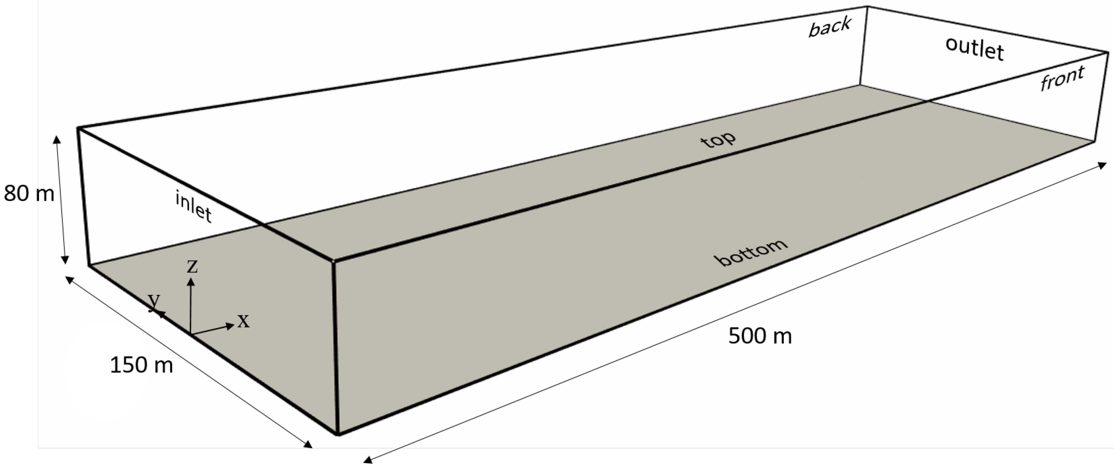
4.1. Computational Domain

The geometry is an empty cuboid with flow along the positive x-direction, as in Figure 9. The dimensions of the domain 500 m × 150 m × 80 m. The dimensions and the grid size were chosen after preliminary studies, which are not presented in this study for brevity. The  domain height was chosen based on the available wind data. The front, back and top boundaries were considered as symmetryPlane, the bottom was considered as wall, and inlet and outlet as patch. Two meshes were considered for the simulation. The domain was first meshed with a small number of cells, and then then refined using the solver’s in-built refineMesh utility. The cells were graded along the z-direction, so that the mesh near the bottom wall was fine, with a nearly uniform aspect-ratio. The mesh consisted of 19,995,000 hexahedral cells.

4.2. Turbulent Inlet

To generate fully turbulent inflow conditions in a cost-efficient way, the Divergence-Free Synthetic Eddy Method (DFSEM) was applied to produce a divergence-free turbulence field directly at the inlet of the computational domain. This approach was introduced by Poletto et al. [46] and represents a consequent development of the so-called Synthetic Eddy Method (SEM), which was proposed earlier by Jarrin et al. [47]. Accordingly, based on the Reynolds decomposition of the velocity field, the velocity fluctuations u i are considered as velocity perturbations caused by N turbulent structures randomly placed within a certain volume of space:
u i ( x i ) = 1 N k = 1 N q 0 ( | r i k | ) | r i k | 3 r i k × α i k ,
where r i k = x i x i k σ k , including x i k as the location of the center of the k-th eddy and the turbulence length-scale σ k calculated at the eddy center. Moreover, Equation (12) consists of a suitable shape function q 0 as well as the eddy intensity α i k , represented by random numbers with zero average. Further information can be found according to the formulation of the DSFEM in [46,48].
The DSFEM requires input parameters to generate the turbulent inflow, namely, the velocity vector, Reynolds stress tensor and integral length scale. To obtain these parameters, wind tunnel experiments were conducted in an atmospheric boundary layer wind tunnel. The  inflow profile was described in a previous validation study [49]; the wind tunnel is described in detail in [50].
Two characteristics of the simulated wind field will be assessed. The first is the vertical profile of the time-averaged velocity in x-direction u x ¯ and its stability throughout the whole domain. The second is a turbulence characteristic, namely, the Reynolds stress R11, which is defined as the time-average of the square of the velocity fluctuations in x-direction: R 11 = u X · u x ¯ , with  u x = u x u x ¯ . As can be seen, R11 is closely related to the turbulence intensity in x-direction. Ux and R11 were chosen because they are considered to be two of the most important characteristics for a modeled windfield in the guidelines for Physical modelling of flow and dispersion processes in the atmospheric boundary layer [51].

4.3. Solver Setup

To simulate the flow field, the validated dynamicKEqn turbulence model was used, with pimpleLPTFoam solver. The flow field was simulated for a period of 400 s without particles. The period of 400 s was chosen, assuming the average wind speed to be 5 m/s, so that the flow passes through the domain four times. Second-order linearUpwind schemes were used for the div(phi,U)and div(phi,k) terms. The case setup and the solver can be found and downloaded in [52] for further use by the reader. The simulation was performed with 420 processors on the SUPERMUC at Leibniz Supercomputing Centre running for 8 h with a maximum Courant number of 1. After 400 s, the particles were injected and the simulation was continued for further 120 s, which then required another 8 h of simulation time. During the particle phase, the results were written out every 5 s. Even though pimpleLPTFoam and MPPICFoam were able to produce similar results, as discussed in Section 5.2, pimpleLPTFoam was chosen as the solver, as it was convenient to use with the turbulentDFSEMInlet boundary condition.

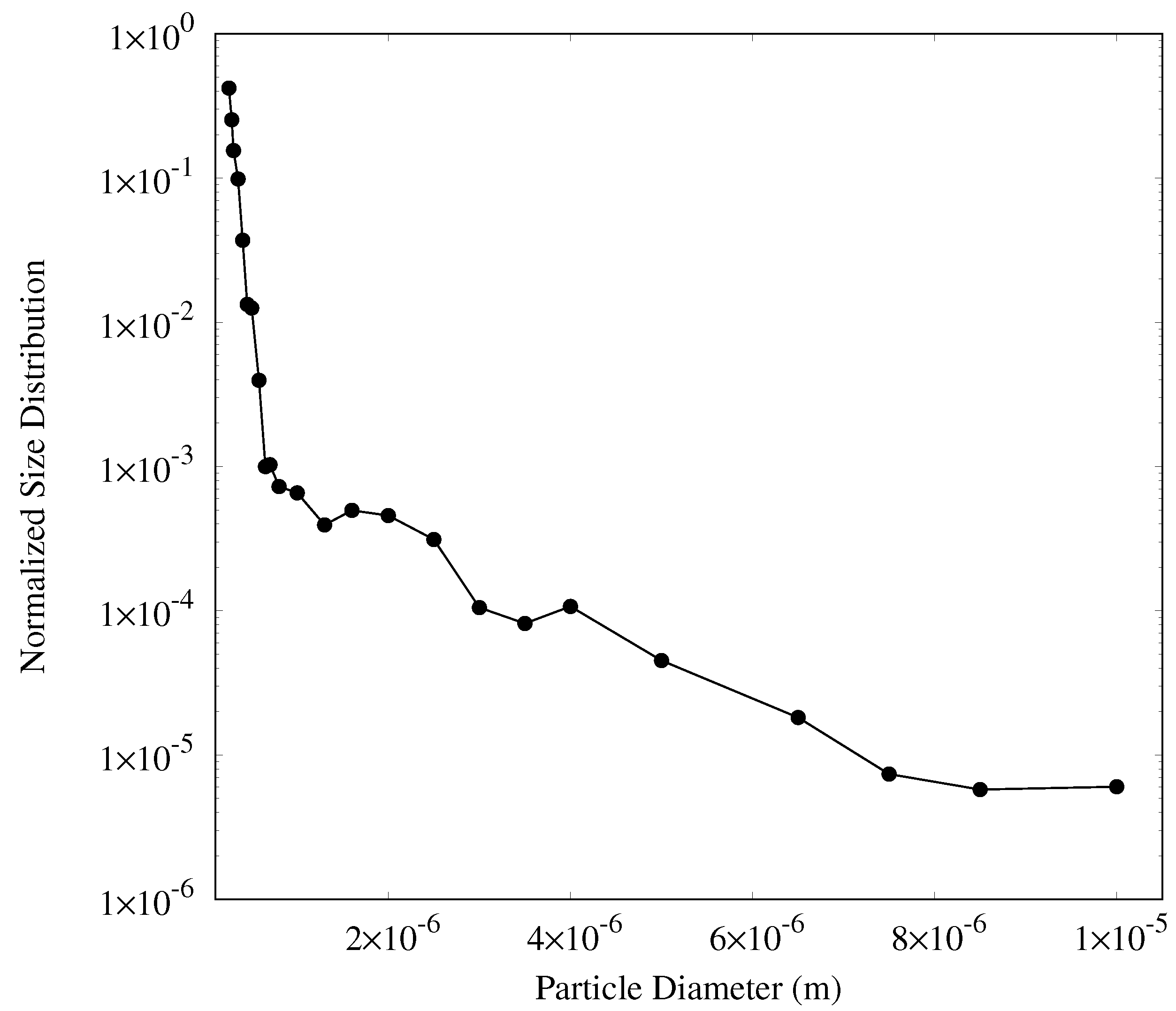
4.4. Particle Properties

The size distribution and density of the particulate matter aerosolized from the manure were obtained from the wind tunnel experiments published in [10,11], where the measured density of the investigated manure was 316 kg/m3, and the density of the aerosolized particulate matter was estimated as 130 kg/m3. The size distribution of the particulate matter was measured and is shown in Figure 10.
In the simulation, the particles were released 50 m downstream the inlet at 1.5 m height. The particles were released from three points at y = −0.25, 0 and 0.25 m. Each second, 400 particles were randomly released from these three points. The particle phase was modelled in one-way coupling since the Stokes number of the particles is less than 1 (2.19 × 10⁻⁶) and the volume fraction is of the order of 1 × 10⁻¹⁵. The particles were modeled with drag and gravitational force, and without collision between the particles. The particle phase was simulated for a period of 120 s, and the spatial distribution of particle concentration in the domain was estimated afterwards. Particles of diameters ranging from 0.25 to 10 μm, with a total of 24 particle sizes, were analyzed at 1012 positions. In the x-direction, the particles were analyzed from x = 50 to x = 500 m for every 10 meters; in y-direction, the particles were analyzed from y = −25 m to y = 25 m for every 5 m; in the z-direction, the particles were analyzed at z = 0.5 m and z = 1.5 m. The regions of analysis were spheres of volume 1 m3.
The obtained particle concentrations were time-averaged for 120 s and summarized based on the particulate matter size. For example, the particle concentration of all sizes less than 1 μm was summed to obtain the particulate matter concentration of PM1. Similarly, the PM2.5 and PM10 concentrations were obtained and plotted, as shown later in Figure 14.

4.5. Results

The results for the particulate matter dispersion from manure application are shown here, with regards to the quality of the simulated wind field, the dispersion of particulate matter, dependent on the diameter and density, and the potential health risks due to air quality.

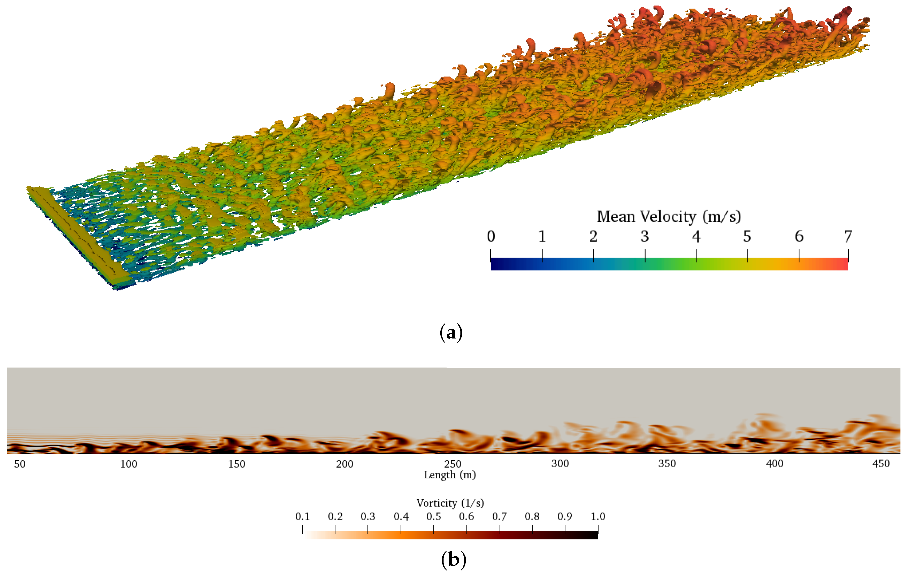
4.5.1. Atmospheric Boundary Layer

Figure 11a shows the instantaneous velocity field of the domain after a 400 s simulation time (shortly before the particles are injected) with iso-contours of the second invariant of the velocity gradient tensor, which is a useful characteristic to display vortex morphology. Figure 11b shows the same velocity field as a detailed 2D view on the XZ-midplane (y = 0) with a height up to 40 m, and the vorticity displayed. It can be seen that a fully turbulent flowfield has evolved, beginning at approximately x = 50 m. With more distance from the inlet, more vorticity is visible in the higher regions, up to 20 m in the vicinity of the outlet, which is probably due to the additional friction from the floor.
Figure 12a shows the vertical velocity profile in x-direction at three different locations, x = 125, 250 and 375 m, and the values that were initially set at the inlet. In the region from the bottom until a height of approximately 40 m, all simulation results fit very well with the initial inlet data, which means a stable velocity profile is created from the inlet to the outlet. In the region from 40 m height up to the top of the domain, the simulated velocities gradually become lower than the inlet velocity, e.g., at a height of 60 m, the three simulated values are around 10 % slower than the inlet velocity at that height. This is due to the influence of the top boundary and could be improved by increasing the height of the domain.
The vertical profile of the Reynolds stress R11 was also stable throughout the domain with a good match with the experimental results for heights up to approximately 25 m. The good agreement of this turbulent characteristic at the first sampling position at x = 125 m indicates, that vortices are correctly produced by theDFSEM generator and transported without decay from the inlet to the outlet. However, for regions above 25 m, higher deviations from the experimental values occur, with an inverse trend. The reason for this might be the geometry of the computational mesh, which is concentrated towards the ground, resulting in smaller cells in the bottom region, and coarser cells with higher aspect ratios towards the top. The sensitivity of the DFSEM turbulence generator on the cell size and geometry should, therefore, be investigated further.

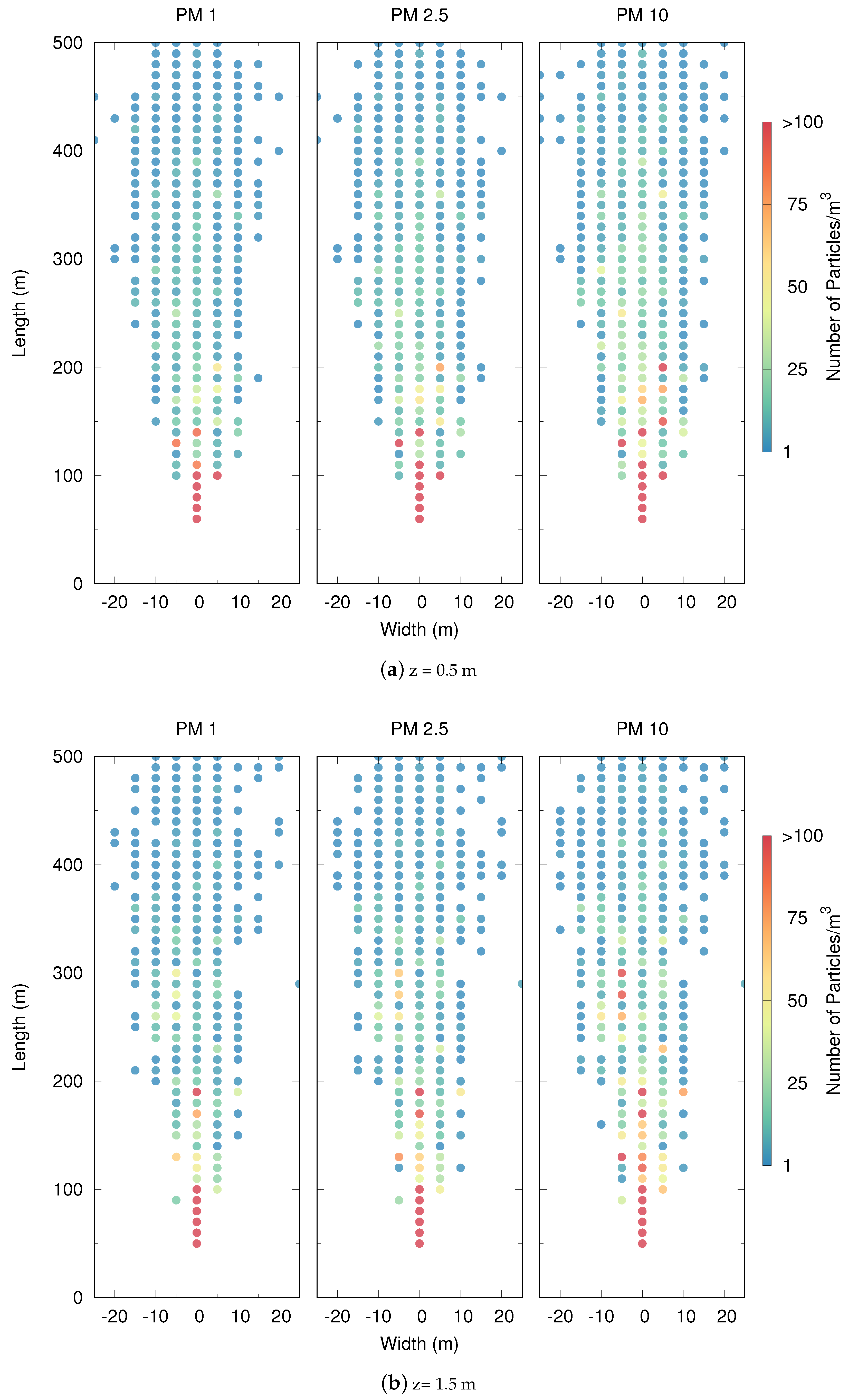
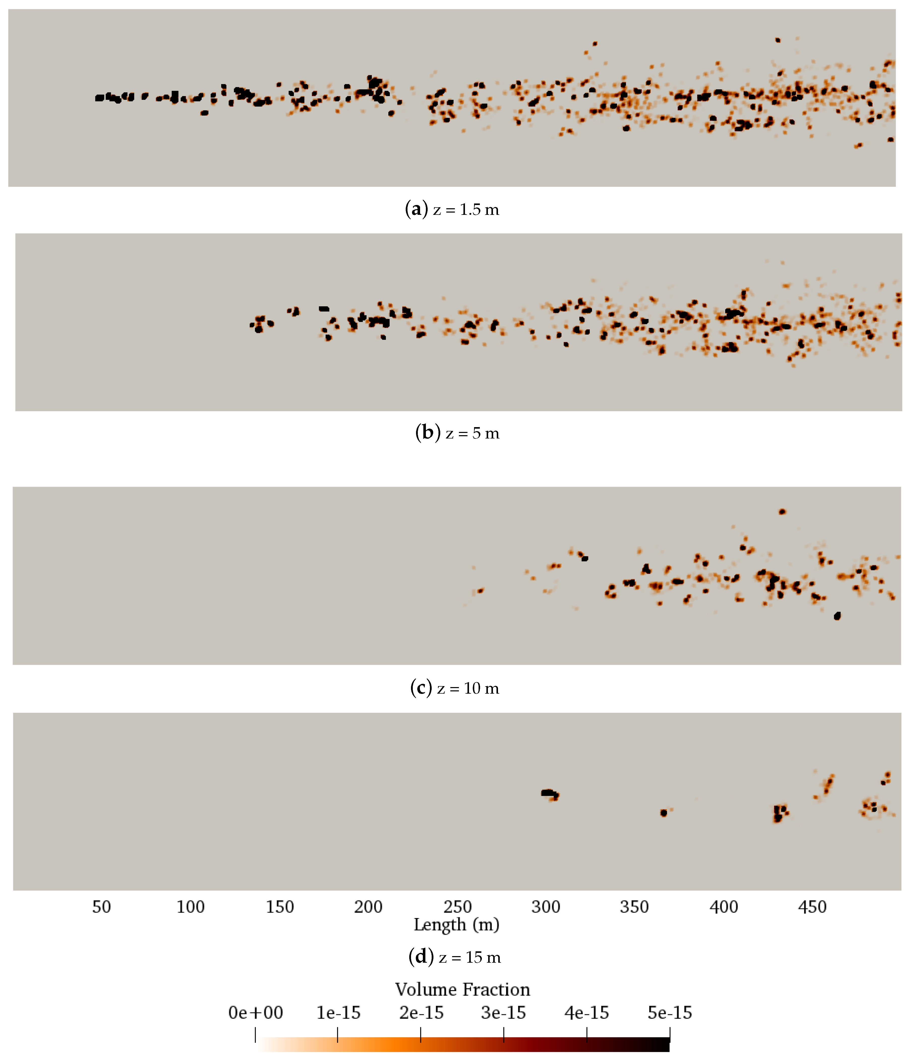
4.5.2. Influence of Size of Particulate Matter

Figure 13 shows the instantaneous dispersion of particles in the domain, 120 s after their injection, and individually displayed for particle diameters of 1 μm (Figure 13a) and 10 μm (Figure 13b). Both particle sizes follow the flow immediately due to the very low Stokes number. A difference between the dispersion of particles according to their size is visible when accounting for their age (which is the duration of stay of a particle in the domain since its respective injection). It can be seen that old particles (age between 80 and 120 s) of size 10 μm have deposited on the ground in the downstream region, beginning from x = 100 m until the outlet. This deposition did not occur for particles with a 1 μm diameter. Here, the oldest visible particles are at the age of around 60 s, which means that all particles of this size are transported directly through the domain. A similar behavior with a faster deposition of particles with larger diameters was also reported in experimental studies of, e.g., [53].
Considering the concentration of particles at z = 0.5 m and z = 1.5 m in Figure 14, in the lower level, particles are evenly detected after x = 100 m, whereas at the higher level, particles are sparsely distributed. Along the line y = −10 m at the lower level, particles could be located from x = 150 m for PM1 and PM2.5, but, at the higher level, they could only be detected after x = 200 m. This behaviour of the particles was mainly due to the turbulent vortices present in the flow field.
Since the source is located at z = 1.5 m, particulate matter could be seen from the source until the end of domain as in Figure 15a, where the PM10 moves straight for a certain distance and then starts to disperse. At z = 1.5 m level, PM10 was dispersed to a width of y = 40 m. From Figure 15, it could be noted that when the height increases, PM10 was detected further away from the source. At z = 5, 10 and 15 m, the particles could be seen only after 125 m, 250 m and 300 m, respectively.

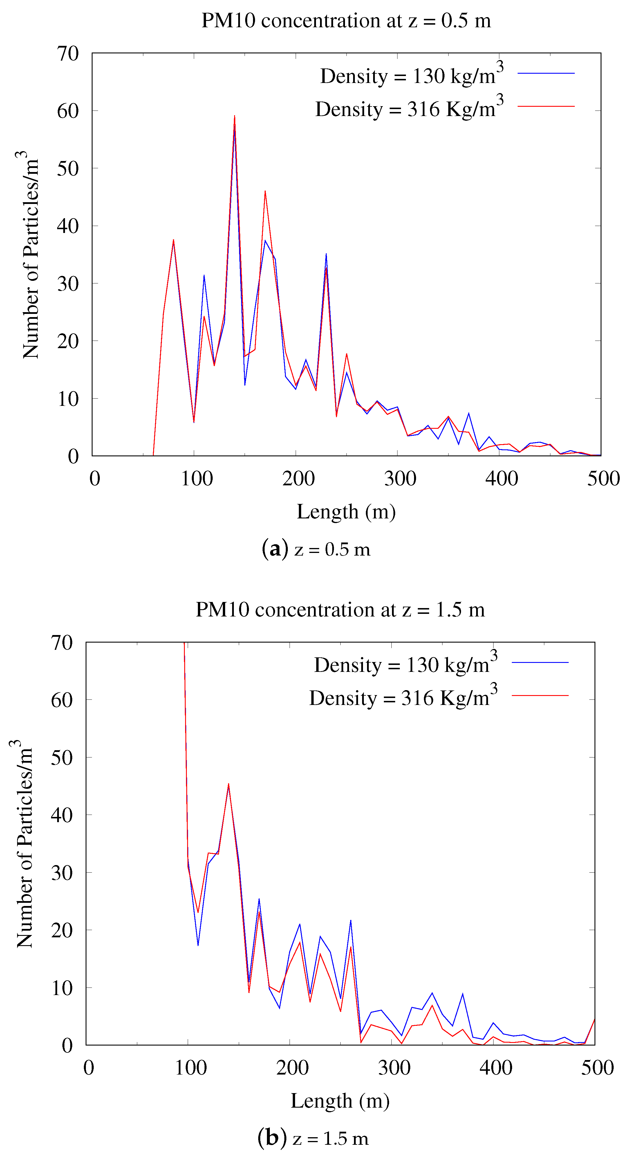
4.5.3. Influence of Density

To investigate the influence of density, the particulate matter with densities 130 kg/m3 and 316.6 kg/m3 were simulated with the same initial conditions and mesh as described before. The time averaged particulate matter concentration was spatially averaged over the y-direction and plotted as in Figure 16. The difference between the PM10 concentrations at z = 0.5 m is small. At x = 70 m, the difference is only 0.7 and similar difference is observed in other points, which are not visible. The concentration of PM10 with 316.6 kg/m3 is high at z = 0.5 m.
A clear trend for the PM10 concentration at z = 1.5 m can be seen for greater distances from the source than approximately 250 m. Here, the PM10 concentrations from the particles with the lower density are always higher than the concentrations from the particles with higher density. On average, after 250 m, at the height of 1.5 m, the concentration of high-density particles was round 50 % less than the concentration of low-density particles. It could be understood that the particles with a lower density tend to spread further than the particles with a higher density, which tend to deposit to the ground.

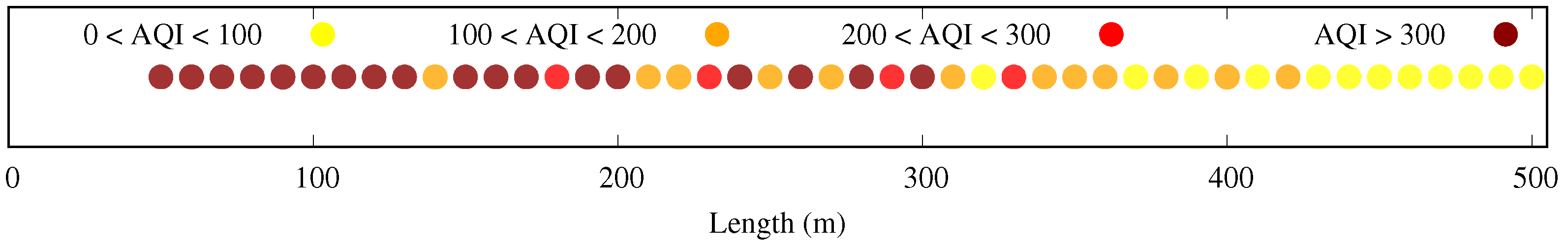
4.5.4. Risk Estimation

The simulated concentrations of particulate matter from the manure application example was used to assess the risk of particulate matter exposure for humans dependent on their distance to the pollutant source. This was done based on the Air Quality Index (AQI) by the USEPA [54]. According to USEPA, the risk is assessed such that AQI < 50 is Good, AQI 51 to 100 is Moderate, AQI 101 to 150 is Unhealthy for sensitive groups, AQI 151 to 200 is Unhealthy, AQI 201 to 300 is Very Unhealthy and AQI > 301 is Hazardous.The spatially averaged particulate matter concentration was converted to μg/m3 by using the density and volume of the particulate matter. For computational cost-effective simulations, the injected particle mass was 0.0066 μg per second. To use the AQI under the assumption of a hazardous environment directly at the source, the simulated concentration results were proportionally increased such that the injected particle mass was 100 μg per second.
Based on the simulation results, the PM10 concentration was classified into four types as in Figure 17. It could be observed from the figure, up to 200 m the AQI is greater than 300, and up to 400 m the AQI is in between 100 and 300 and beyond 400 m the AQI is less than 100.

5. Discussion

5.1. Flowfield

Regarding the turbulence models, the equilibrium-assumption models kEqn and Smagorinsky were not efficient in reproducing the results, which is clearly due to their inability to handle the transition by these models, as discussed in [36]. However, the solver was able to simulate a very well-matching velocity field in the investigated region with the two non-equilibrium SGS turbulence models WALE and dynamicKEqn. Larger deviations were only seen in the near-wall regions. This may be due to the presence of y + values in the buffer region. Even though nutUSpaldingWallFunction was used to compensate the y + values, a better mesh refinement could have resulted in more accurate results and should be investigated in further simulations. Alternatively, so-called detached eddy simulations (DES, a mixed approach of RANS for simulating the near-wall flow, and LES for simulating the non-wall-affected flow) could improve the wall-near results and simultaneously reduce computational effort, which is described, e.g., in [36].
Nevertheless, the LES results obtained in this study were more accurate than the results from the simulations, which were additionally conducted in the experimental study by Gromke et al. [35], who used an RANS approach. At the points that were used for the mesh convergence study, their published results had an error of round 60%, while the LES dynamicKEqn model showed an error of only 4%. This is a good indicator for the advantages of transient LES over steady-state RANS in the context of complex flows, which will be discussed further in Section 5.4. The dynamicKEqn model was also validated in a previous study to simulate the flow inside a naturally ventilated dairy barn and was found to perform very well for the most important characteristics [55]. Future studies on the coupling of indoor and outdoor flow will, therefore, focus on this turbulence model.

5.2. Particle Dispersion

The results for validating the particle dispersion showed no differences between the two investigated solvers for the solid phase. The simulations were obviously less sensitive to the Lagrangian solver for the particle transport, and more attention should be paid to the accurate solution of the flow field, especially the turbulent characteristics. Larger discrepancies between experimental an simulation data for the particle concentrations were found in the lower region of the computational domain, which are most likely a result of the velocity overprediction at the inlet jet, when LES was applied. We tested several different meshes, wall functions and SGS models (for brevity, not shown in this study) with no improvement in the results for the velocity field. Probably, the application of well-defined velocity boundary conditions (in terms of time series) at the inlet would improve the velocity field. Unfortunately, the study for the validation of the particle dispersion did not provide information on the inflow characteristics of the test room. This was carried out under nearly laminar conditions with a Reynolds number of ≈1200. An experiment in a fully turbulent flow, with documented inlet velocity characteristics, would likely have resulted in a more accurate prediction of the flow field and, therefore, of the particle dispersion. Overall, an acceptable match between the experimental results and the simulations results can be stated, with a good recapturing of the general trend and a good match in the upper third of the domain. However, at this stage of validation, the investigated solvers PimpleLPTFoam and MPPICFoam is rather reliable for an assessment of trends (e.g., general effectiveness of flow barriers) than for the derivation of absolute values as needed, e.g., in civil protection applications. A bottleneck here is the lack of high-quality datasets under realistic turbulent conditions, which can be used for validatation.

5.3. Application Example

The DFSEM inlet boundary condition was able to create a vertical velocity profile, which matched the experimental data very well. The profile was stable throughout the domain, which is important for the dispersion studies and indicates a fully developed turbulent boundary layer from the beginning. This is usually achieved only after a longer simulated inflow section with natural turbulence generation or a recycling strategy, where the velocity values from the outlet are mapped and superimposed on the inlet [56,57,58]. These strategies require a considerable amount of computational effort. By using the synthetic turbulence generator DFSEM, this effort was not required; hence, this boundary condition is a promising tool for further efficient investigations of atmospheric dispersion processes. Up to a height of 25 m (which covers the usual region of interest when investigating near source immissions) the Reynolds stresses R11 were in good agreement with the experimentally derived initial conditions throughout the domain. However, for regions above this height, larger deviations were seen, which could lead to inaccurate dispersion simulations. These deviations are likely due to an interaction between the DFSEM and a non-uniform mesh. Hence, the sensitivity of generated eddies on the grid aspect ratio should be further investigated on unstructured meshes.
The simulations of the particle phase in the validated flow field showed two main trends for the dispersion of PM. First, particles with larger diameters tend to sediment earlier on the bottom and are not spread as widely as particles with smaller diameters. This was previously reported in experimental studies e.g., in [53,59]. Second, the density of the PM had a strong influence on the dispersion. The concentrations of particles with a higher density after a certain distance were always lower than the ones with a lower density. This can be explained by the interaction between drag and gravitational forces, where the latter are greater for particles with a higher density; hence, these particles tend to sediment earlier, as described by Sehmel [60]. The ability of the investigated solver to reproduce this behavior is an important feature, because it shows the potential for further simulations of varying sources of PM (e.g., from different types of fertilizers) and their respective immission impact in the near field.

5.4. Performance: Cost-Benefit Ratio

It is obvious that the transient large-eddy simulations presented in this study require more computing capacities than the usually applied steady-state RANS simulations. However, we believe the inherent advantages of LES compensate for this drawback. In general, for complex turbulent flows with flow separation and transitional effects (as is typical for the flowfield in the near field of animal housing systems), LES are superior to RANS, because the main portions of the turbulence are directly computed and not modeled, as discussed, e.g., in [19,61]. This good applicability for complex flows can also be confirmed by our results for the street canyon flow discussed in Section 5.1. For an efficient use of LES in agricultural applications, which are characterized by usually large dimensions with several scales of interest, the use of massive parallel processing (use of large computer clusters/supercomputers) is indispensable. One or two decades ago, this would make the practical implementation of LES difficult or nearly impossible. However, in recent years, external cloud computing services became more popular, resulting in a decline in costs for simulation time, so that even with a smaller budget, large-scale simulations can be carried out. The use of open-source solvers saves money for the sometimes exorbitant high license fees for proprietary solvers in parallel computing [55], and these saved resources are usually higher than the fees required to rent external simulation time.

6. Conclusions and Outlook

The goals of this study, which were formulated in Section 1, could be fulfilled. An open source solver for the simulation of PM dispersion was validated with respect to the velocity field, the transport of particles, and the generation of synthetic turbulence, and this was demonstrated with an example application of manure on a field.
It could be shown that a precise analysis of the spatial distribution of PM concentration is possible, with distinguishing between certain particle properties such as size, density or age. This is very useful for the further use of the solver in risk assessment in the near source emmission area. At this stage of validation, the investigated solver can already be used to investigate the impact of measures, such as, e.g., flow barriers, on the particle concentrations in terms of relative changes. To improve the validation process of the particle transport solver, high-resolution measurements of PM dispersion under realistic conditions are needed for validation datasets. Experiments should be designed and carried out to generate these datasets.
However, the results discussed here are valid for dry conditions with a neutral stratification. Particle dispersion in atmospheric flows is usually influenced by humidity effects (coagulation or evaporation), and also by thermal buoyancy in case of non-neutral stratification. Simulations with the tested solver with additional humidity–particle interaction and solving the temperature field will, therefore, improve the results and be the subject of further investigations. Additionally, the presence of pathogens in the PM could be taken into consideration by giving the particles ’pathogen-like’ properties, so that the particles are active for a specific period of time and interact with environmental conditions such as UV-Radiation. These extensions can be added to the model by including already existing libraries, such as the OpenFOAM software package.
Given that, the model has the potential for a powerful tool, especially to accurately simulate near-source pollution, e.g., in case of a disease outbreak with pathogen-laden dust in a certain barn, the risk of contamination of the neighboring barns can be assessed, which might lead to less culling of the unaffected animals.

Author Contributions

Conceptualization: D.J., S.S. and T.A.; methodology: D.J., S.S.; software: D.J., S.S.; formal analysis: D.J., R.K., S.H., T.A.; investigation: D.J., S.S., R.K.; data curation: S.S., D.J.; writing–original draft preparation: S.S., D.J., R.K., S.H., T.A.; writing–review and editing: D.J., R.K., S.H.; visualization: D.J., S.S.; supervision: T.A. All authors have read and agreed to the published version of the manuscript.

Funding

This research was partly funded by the Leibniz Association, Berlin, Germany, within the Senate committee competition (SAW)2017 (grant number: SAW-2017-DSMZ-2) and supported by the Leibniz Research Alliance “INFECTIONS ’21”.

Acknowledgments

The authors gratefully acknowledge the Gauss Centre for Supercomputing e.V. (www.gauss-centre.eu accessed on 5 September 2021) for funding this project by providing computing time on the GCS Supercomputer SuperMUC-NG at Leibniz Supercomputing Centre (www.lrz.de accessed on 5 September 2021).

Conflicts of Interest

The authors declare no conflict of interest.

Abbreviations

The following abbreviations are used in this manuscript:
ARTAerosols and reactive trace gases
AQIAir quality index
CFDComputational fluid dynamics
COSMOConsortium for Small Scale Modelling Europe
DEMDetached-eddy simulation
DFSEMDivergence-free synthetic eddy method
DPMDiscrete parcel method
DWDGerman Weather Service
LDALaser Doppler anemometry
LESLarge eddy simulation
LPTLagrangian particle tracking
MPPICMultiphase particle-in-cell method
OpenFOAMOpen Source Field Operation and Manipulation
PDAPhase Doppler anemometry
PISOPressure implicit with splitting of operator
PMParticulate matter
SEMSynthetic eddy method
SGSSubgrid scale
SIMPLESemi-implicit method for pressure linked equations
TKETurbulence kinetic energy
(U)RANS(Unsteady) Reynolds-averaged Navier-Stokes equations
USEPAUnited States Environmental Protection Agency
UVUltraviolet
WALEWall-adapting local eddy-viscosity model

References

  1. Arslan, S.; Aybek, A. Particulate Matter Exposure in Agriculture. In Air Pollution; Haryanto, B., Ed.; IntechOpen: Rijeka, Croatia, 2012; Chapter 3. [Google Scholar]
  2. World Health Organisation. Burden of Disease from Ambient Air Pollution; Global Health Observatory Data; World Health Organisation: Geneva, Switzerland, 2014; Available online: https://www.who.int/airpollution/data/AAP_BoD_results_March2014.pdf (accessed on 5 September 2021).
  3. Aarnink, A.; Ellen, H. Processes and Factors Affecting Dust Emissions from Livestock Production. In How to Improve Air Quality; Wageningen University & Research: Wageningen, The Netherlands, 2007; Available online: https://research.wur.nl/en/publications/processes-and-factors-affecting-dust-emissions-from-livestock-pro (accessed on 5 September 2021).
  4. Lelieveld, J.; Evans, J.S.; Fnais, M.; Giannadaki, D.; Pozzer, A. The contribution of outdoor air pollution sources to premature mortality on a global scale. Nature 2015, 525, 367–371. [Google Scholar] [CrossRef] [PubMed]
  5. Bundesamt, S. Wirtschaftsduenger Tierischer Herkunft in Landwirtschaftlichen Betrieben/Agrarstrukturerhebung-Fachserie 3 Reihe 2.2.2-2016; Statistisches Bundesamt: Wiesbaden, Germany, 2017. Available online: https://www.destatis.de/DE/Themen/Branchen-Unternehmen/Landwirtschaft-Forstwirtschaft-Fischerei/Produktionsmethoden/Publikationen/Downloads-Produktionsmethoden/wirtschaftsduenger-2030222169005.html (accessed on 5 September 2021).
  6. Funk, R.; Reuter, H.I.; Hoffmann, C.; Engel, W.; Öttl, D. Effect of moisture on fine dust emission from tillage operations on agricultural soils. Earth Surf. Process. Landf. J. Br. Geomorphol. Res. Group 2008, 33, 1851–1863. [Google Scholar] [CrossRef]
  7. Maffia, J.; Dinuccio, E.; Amon, B.; Balsari, P. PM emissions from open field crop management: Emission factors, assessment methods and mitigation measures—A review. Atmos. Environ. 2020, 226, 117381. [Google Scholar] [CrossRef]
  8. Takai, H.; Pedersen, S.; Johnsen, J.O.; Metz, J.; Koerkamp, P.G.; Uenk, G.; Phillips, V.; Holden, M.; Sneath, R.; Short, J.; et al. Concentrations and emissions of airborne dust in livestock buildings in Northern Europe. J. Agric. Eng. Res. 1998, 70, 59–77. [Google Scholar] [CrossRef] [Green Version]
  9. Cambra-López, M.; Aarnink, A.J.; Zhao, Y.; Calvet, S.; Torres, A.G. Airborne particulate matter from livestock production systems: A review of an air pollution problem. Environ. Pollut. 2010, 158, 1–17. [Google Scholar] [CrossRef] [PubMed]
  10. Kabelitz, T.; Ammon, C.; Funk, R.; Münch, S.; Biniasch, O.; Nübel, U.; Thiel, N.; Rösler, U.; Siller, P.; Amon, B.; et al. Functional relationship of particulate matter (PM) emissions, animal species, and moisture content during manure application. Environ. Int. 2020, 143, 105577. [Google Scholar] [CrossRef] [PubMed]
  11. Kabelitz, T.; Biniasch, O.; Ammon, C.; Nübel, U.; Thiel, N.; Janke, D.; Swaminathan, S.; Funk, R.; Münch, S.; Rösler, U.; et al. Particulate matter emissions during field application of poultry manure-The influence of moisture content and treatment. Sci. Total Environ. 2021, 780, 146652. [Google Scholar] [CrossRef]
  12. Mostafa, E.; Nannen, C.; Henseler, J.; Diekmann, B.; Gates, R.; Buescher, W. Physical properties of particulate matter from animal houses—Empirical studies to improve emission modelling. Environ. Sci. Pollut. Res. 2016, 23, 12253–12263. [Google Scholar] [CrossRef] [PubMed]
  13. McEachran, A.D.; Blackwell, B.R.; Hanson, J.D.; Wooten, K.J.; Mayer, G.D.; Cox, S.B.; Smith, P.N. Antibiotics, bacteria, and antibiotic resistance genes: Aerial transport from cattle feed yards via particulate matter. Environ. Health Perspect. 2015, 123, 337–343. [Google Scholar] [CrossRef] [Green Version]
  14. Ferziger, J.H.; Perić, M.; Street, R.L. Computational Methods for Fluid Dynamics; Springer: Berlin/Heidelberg, Germany, 2002; Volume 3. [Google Scholar]
  15. Van Dop, H.; Nieuwstadt, F.; Hunt, J. Random walk models for particle displacements in inhomogeneous unsteady turbulent flows. Phys. Fluids 1985, 28, 1639–1653. [Google Scholar] [CrossRef]
  16. Nimmatoori, P.; Kumar, A. Dispersion Modeling of Particulate Matter in Different Size Ranges Releasing from a Biosolids Applied Agricultural Field Using Computational Fluid Dynamics. Adv. Chem. Eng. Sci. 2021, 11, 180–202. [Google Scholar] [CrossRef]
  17. Quinn, A.; Wilson, M.; Reynolds, A.; Couling, S.; Hoxey, R. Modelling the dispersion of aerial pollutants from agricultural buildings—An evaluation of computational fluid dynamics (CFD). Comput. Electron. Agric. 2001, 30, 219–235. [Google Scholar] [CrossRef]
  18. Wang, M.; Lin, C.H.; Chen, Q. Advanced turbulence models for predicting particle transport in enclosed environments. Build. Environ. 2012, 47, 40–49. [Google Scholar] [CrossRef]
  19. Blocken, B. LES over RANS in building simulation for outdoor and indoor applications: A foregone conclusion? In Building Simulation; Springer: Berlin/Heidelberg, Germany, 2018; Volume 11, pp. 821–870. [Google Scholar]
  20. Deetz, K.; Klose, M.; Kirchner, I.; Cubasch, U. Numerical simulation of a dust event in northeastern Germany with a new dust emission scheme in COSMO-ART. Atmos. Environ. 2016, 126, 87–97. [Google Scholar] [CrossRef]
  21. Vogel, B.; Vogel, H.; Bäumer, D.; Bangert, M.; Lundgren, K.; Rinke, R.; Stanelle, T. The comprehensive model system COSMO-ART–Radiative impact of aerosol on the state of the atmosphere on the regional scale. Atmos. Chem. Phys. 2009, 9, 8661–8680. [Google Scholar] [CrossRef] [Green Version]
  22. Faust, M.; Wolke, R.; Münch, S.; Funk, R.; Schepanski, K. A new Lagrangian in-time particle simulation module (Itpas v1) for atmospheric particle dispersion. Geosci. Model Dev. 2021, 14, 2205–2220. [Google Scholar] [CrossRef]
  23. Smagorinsky, J. General circulation experiments with the primitive equations. Mon. Wea. Rev. 1963, 91, 99–164. [Google Scholar] [CrossRef]
  24. Nicoud, F.; Ducros, F. Subgrid-scale stress modelling based on the square of the velocity gradient tensor. Flow Turbul. Combust. 1999, 62, 183–200. [Google Scholar] [CrossRef]
  25. Yoshizawa, A.; Horiuti, K. A statistically-derived subgrid-scale kinetic energy model for the large-eddy simulation of turbulent flows. J. Phys. Soc. Jpn. 1985, 54, 2834–2839. [Google Scholar] [CrossRef]
  26. Yoshizawa, A. Statistical theory for compressible turbulent shear flows, with the application to subgrid modeling. Phys. Fluids 1986, 29, 2152–2164. [Google Scholar] [CrossRef]
  27. Kim, W.W.; Menon, S. A new dynamic one-equation subgrid-scale model for large eddy simulations. In 33rd Aerospace Sciences Meeting and Exhibit; Aerospace Research Central: Reno, NV, USA, 1995; p. 356. [Google Scholar]
  28. Dyna, C. Multi-Phase Flows and Discrete Phase Models. Available online: http://www.cfdyna.com/Home/of_multiPhase.html (accessed on 5 September 2021).
  29. Michaelides, E.E.; Crowe, C.T.; Schwarzkopf, J.D. (Eds.) Multiphase Flow Handbook; Taylor & Francis Inc.: Abingdon, UK, 2016. [Google Scholar]
  30. Putnam, A. Integrable form of droplet drag coefficient. ARS J. 1961, 31, 1467–1470. [Google Scholar]
  31. Gidaspow, D. Multiphase Flow and Fluidization: Continuum and Kinetic Theory Descriptions; Academic Press, Inc.: Cambridge, MA, USA, 1994. [Google Scholar]
  32. Wen, Y.; Yu, Y. Mechanics of fluidization. Chem. Eng. Prog. Symp. Ser. 1966, 162, 100–111. [Google Scholar]
  33. Cameron, T.; Alexander, Y.; Foss, J. Springer Handbook of Experimental Fluid Mechanics; Springer: Berlin/Heidelberg, Germany, 2007; p. 289. [Google Scholar]
  34. Elghobashi, S. On predicting particle-laden turbulent flows. Appl. Sci. Res. 1994, 52, 309–329. [Google Scholar] [CrossRef]
  35. Gromke, C.; Buccolieri, R.; Di Sabatino, S.; Ruck, B. Dispersion study in a street canyon with tree planting by means of wind tunnel and numerical investigations–evaluation of CFD data with experimental data. Atmos. Environ. 2008, 42, 8640–8650. [Google Scholar] [CrossRef]
  36. De Villiers, E. The Potential of Large Eddy Simulation for the Modeling of Wall Bounded Flows; Imperial College of Science, Technology and Medicine: London, UK, 2006. [Google Scholar]
  37. Liu, F. A Thorough Description of How Wall Functions Are Implemented in OpenFOAM; Technical Report; Chalmers University of Technology: Gothenburg, Sweden, 2017. [Google Scholar]
  38. Issa, R.I. Solution of the implicitly discretised fluid flow equations by operator-splitting. J. Comput. Phys. 1986, 62, 40–65. [Google Scholar] [CrossRef]
  39. Patankar, S.V.; Spalding, D.B. A calculation procedure for heat, mass and momentum transfer in three-dimensional parabolic flows. In Numerical Prediction of Flow, Heat Transfer, Turbulence and Combustion; Elsevier: Amsterdam, The Netherlands, 1983; pp. 54–73. [Google Scholar]
  40. Holzmann, T. Mathematics, Numerics, Derivations and OpenFOAM®; Holzmann CFD: Augsburg, Germany, 2016; pp. 95–112. [Google Scholar] [CrossRef]
  41. The OpenFOAM Foundation. OpenFOAM User Guide Version 4.0. 2016. Available online: https://cfd.direct/openfoam/user-guide-v4/ (accessed on 5 September 2021).
  42. Chen, F.; Simon, C.; Lai, A.C. Modeling particle distribution and deposition in indoor environments with a new drift–flux model. Atmos. Environ. 2006, 40, 357–367. [Google Scholar] [CrossRef]
  43. Andrews, M.J.; O’Rourke, P.J. The multiphase particle-in-cell (MP-PIC) method for dense particulate flows. Int. J. Multiph. Flow 1996, 22, 379–402. [Google Scholar] [CrossRef]
  44. Kasper, R.; Turnow, J.; Kornev, N. Numerical modeling and simulation of particulate fouling of structured heat transfer surfaces using a multiphase Euler-Lagrange approach. Int. J. Heat Mass Transf. 2017, 115, 932–945. [Google Scholar] [CrossRef]
  45. Kasper, R.; Turnow, J.; Kornev, N. Multiphase Eulerian–Lagrangian LES of particulate fouling on structured heat transfer surfaces. Int. J. Heat Fluid Flow 2019, 79, 108462. [Google Scholar] [CrossRef]
  46. Poletto, R.; Craft, T.; Revell, A. A new divergence free synthetic eddy method for the reproduction of inlet flow conditions for LES. Flow Turbul. Combust. 2013, 91, 519–539. [Google Scholar] [CrossRef]
  47. Jarrin, N.; Prosser, R.; Uribe, J.C.; Benhamadouche, S.; Laurence, D. Reconstruction of turbulent fluctuations for hybrid RANS/LES simulations using a synthetic-eddy method. Int. J. Heat Fluid Flow 2009, 30, 435–442. [Google Scholar] [CrossRef] [Green Version]
  48. Bex, C.C.; Pinon, G.; Slama, M.; Gaston, B.; Germain, G.; Rivoalen, E. Lagrangian Vortex computations of turbine wakes: Recent improvements using Poletto’s Synthetic Eddy Method (SEM) to account for ambient turbulence. J. Phys. Conf. Ser. 2020, 1618, 062028. [Google Scholar] [CrossRef]
  49. Saha, C.K.; Yi, Q.; Janke, D.; Hempel, S.; Amon, B.; Amon, T. Opening Size Effects on Airflow Pattern and Airflow Rate of a Naturally Ventilated Dairy Building—A CFD Study. Appl. Sci. 2020, 10, 6054. [Google Scholar] [CrossRef]
  50. Janke, D.; Yi, Q.; Thormann, L.; Hempel, S.; Amon, B.; Nosek, Š.; Van Overbeke, P.; Amon, T. Direct Measurements of the Volume Flow Rate and Emissions in a Large Naturally Ventilated Building. Sensors 2020, 20, 6223. [Google Scholar] [CrossRef]
  51. VDI. Environmental Meteorology-Physical Modelling of Flow and Dispersion Processes in the Atmospheric Boundary Layer-Application of Wind Tunnels; Guideline; Verein Deutscher Ingenieure: Duesseldorf, Germany, 2000. [Google Scholar]
  52. Janke, D.; Swaminathan, S.; Hempel, S.; Kasper, R.; Amon, T. Sample Case Files for the Particulate Matter Dispersion Modeling in Agricultural Applications. 2021. Available online: https://github.com/ssacfd/ATB_particletransport (accessed on 5 September 2021).
  53. Lin, J.J.; Noll, K.E.; Holsen, T.M. Dry deposition velocities as a function of particle size in the ambient atmosphere. Aerosol Sci. Technol. 1994, 20, 239–252. [Google Scholar] [CrossRef] [Green Version]
  54. United States Environmental Protection Agency. Air Quality Guide for Particle Pollution. 2015. Available online: https://www.airnow.gov/publications/air-quality-index/air-quality-guide-for-particle-pollution/ (accessed on 5 September 2021).
  55. Janke, D.; Caiazzo, A.; Ahmed, N.; Alia, N.; Knoth, O.; Moreau, B.; Wilbrandt, U.; Willink, D.; Amon, T.; John, V. On the feasibility of using open source solvers for the simulation of a turbulent air flow in a dairy barn. Comput. Electron. Agric. 2020, 175, 105546. [Google Scholar] [CrossRef]
  56. Nozawa, K.; Tamura, T. Simulation of rough-wall turbulent boundary layer for LES inflow data. In Second Symposium on Turbulence and Shear Flow Phenomena; Begel House Inc.: Danbury, CT, USA, 2001. [Google Scholar]
  57. Nozawa, K.; Tamura, T. Large eddy simulation of the flow around a low-rise building immersed in a rough-wall turbulent boundary layer. J. Wind Eng. Ind. Aerodyn. 2002, 90, 1151–1162. [Google Scholar] [CrossRef]
  58. Lund, T.S.; Wu, X.; Squires, K.D. Generation of turbulent inflow data for spatially-developing boundary layer simulations. J. Comput. Phys. 1998, 140, 233–258. [Google Scholar] [CrossRef] [Green Version]
  59. Esmen, N.A.; Corn, M. Residence time of particles in urban air. Atmos. Environ. (1967) 1971, 5, 571–578. [Google Scholar] [CrossRef]
  60. Sehmel, G.A. Particle eddy diffusivities and deposition velocities for isothermal flow and smooth surfaces. Aerosol Sci. 1973, 4, 125–138. [Google Scholar] [CrossRef]
  61. Van Buggenhout, S.; Van Brecht, A.; Özcan, S.E.; Vranken, E.; Van Malcot, W.; Berckmans, D. Influence of sampling positions on accuracy of tracer gas measurements in ventilated spaces. Biosyst. Eng. 2009, 104, 216–223. [Google Scholar] [CrossRef]
Figure 1. Structure of the study and illustration of the work- and information flow.
Agronomy 11 02246 g001
Figure 2. Geometry for flow field validation. (a) Overview of the computational domain. (b) Detailed view on the cross section of the two buildings forming a street canyon.
Agronomy 11 02246 g002
Figure 3. Mesh convergence study for the flow field validation. The three measurement points from the experiment of [35] were located on a horizontal line in the street canyon on a height of 0.7 H. The values on the ordinate are the normalized velocities in z-direction, with UH as the reference velocity at the inlet on the reference height H. Experimental data from [35], Elsevier, 2008.
Agronomy 11 02246 g003
Figure 4. Comparison of simulation and experimental results for four different subgrid scale turbulence models. (a,b) show the static models, (c,d) the dynamic models. The normalized vertical velocity, with UH as a reference, is shown, which is the inlet velocity at height H. The contours from the experiment are plotted as solid lines and those from simulations as dotted lines, where colors indicate the velocity values.
Agronomy 11 02246 g004aAgronomy 11 02246 g004b
Figure 5. Geometry and mesh for particle phase validation.
Agronomy 11 02246 g005
Figure 6. Comparison of the vertical profiles for the velocity in x-direction. Dots and dashed black lines were formed with data from the experiment of [42], Elsevier, 2006. Red lines are the simulated velocities from the RANS approach, green lines are the time-averaged results from the LES approach.
Agronomy 11 02246 g006
Figure 7. Particle phase at different times (LES—(ad) and URANS (eh)).
Agronomy 11 02246 g007
Figure 8. Comparison of measured and simulated particle concentrations with data from the experiment of [42]. The particle concentration values were normalized with the measured particle concentrations at the inlet of the test room or the computational domain. For the simulations with the two solvers PimpleLPTFoam and MPPICFoam, particle concentrations were computed as the time average of 1800 s simulation time. Experimental data from [42], Elsevier, 2006.
Agronomy 11 02246 g008
Figure 9. Sketch of the domain used for the simulation of the application example. Particles were injected at x = 50 m at three different lateral points y = [−0.25, 0, 0.25] m at a height of 1.5 m.
Agronomy 11 02246 g009
Figure 10. Particle size distribution injected in the application example. The size distribution was obtained from experiments with aerosolized manure in a wind tunnel, as described in [10].
Agronomy 11 02246 g010
Figure 11. View on the instantaneous flowfield after 400 s of simulation. (a) shows the iso-contours for Q = 0.01 s−2, which is the 2nd invariant of the velocity gradient tensor. Surface coloring is carried out in accordance with mean velocity, as shown in the color bar. (b) shows the vorticity of the flowfield after 400 s on a section on the XZ-plane at y = 0, with a height up to z = 40 m.
Agronomy 11 02246 g011
Figure 12. Development of the vertical profiles of (a) velocity, and (b) Reynolds stress R11 at four different locations along the domain in x-direction. Colored lines are the simulation results and time-averaged over 400 s. Black dots are values set at the inlet, derived from atmospheric boundary layer wind tunnel experiments [49].
Agronomy 11 02246 g012
Figure 13. Spread of particles at 120 s from x = 50 m to x = 200 m (Front view with x axis along horizontal and z axis along vertical). The coloring indicates the age of the particles.
Agronomy 11 02246 g013
Figure 14. PM1, PM2.5 and PM10 concentration time averaged over 120 s (Density = 316.6 kg/m3).
Agronomy 11 02246 g014
Figure 15. Volume fraction of PM10 for different heights at 120 s (top view of the domain with x axis along horizontal and y axis along vertical).
Agronomy 11 02246 g015
Figure 16. PM10 concentration time averaged over 120 s and spatially averaged over y-direction.
Agronomy 11 02246 g016
Figure 17. Risk estimation based on PM10 concentration.
Agronomy 11 02246 g017
Table 1. y + values for the walls in buildings A and B.
FineMediumCoarse
Min0.440.711.42
Max61.8079.76167.71
Avg10.9413.0425.28
Publisher’s Note: MDPI stays neutral with regard to jurisdictional claims in published maps and institutional affiliations.

