Abstract
Full-electric boats are an expression of recent advancements in the area of vessel electrification. The installed batteries can suffer from poor cold-start performance, especially in the frigid season and at higher latitudes, leading to driving power limitations immediately after startup. At state, the leading solution is to adopt a dedicated heater placed on the common cooling/heating circuit; this implies poor volume, weight, and cost figures, given the very limited duty cycle of such a part. The Heater-in-Converter (HiC) technology allows removing this specialized component, exploiting the power electronics converters already available on board: HiC modulates their efficiency to produce valuable heat (pseudo-cogeneration). In this work, we use the model-based approach to design this system, which requires heating power minimization to fulfill power electronics limitations, while guaranteeing the user-expected startup time to full power. A multistage model is used to get the yearly vessel temperature distribution from latitude information and some additional data. Then, a lumped parameter for the cooling/heating circuit is used to determine the minimum required power as a function of the properties of the thermal interface material used for the battery coupling. The design is validated on a 1:5 test bench (battery power and energy), which demonstrates how the technology can be to scaled up to also fit different boats and battery sizes.
1. Introduction
The electrification of vessels and other marine vehicles is gaining increasingly more importance to reduce sea pollution, especially in near-shore areas. This is one of the key points of the green maritime transport line of the European Green Deal [1], and many efforts are devoted both to ship development [2] and to the adaption of port infrastructure [3]. Sustaining this major shift in the marine vehicle architecture requires efforts in various areas [4], with battery-based energy storage systems being one topic of paramount importance [5]. High-density Li-ion batteries experience poor performance at low temperatures [6,7]; therefore, specific heating systems are a key enabling technology (KET) for electrified boats and vehicles [8].
In full-electric boats, no internal combustion engine (ICE) exists, so resistive heaters are used to bring batteries to their desired optimal working point from a cold-start condition; this point is the temperature at which the battery is able to source its nominal design power and where overload is safer, i.e., the energy storage system tolerates higher currents without appreciable degradation of its lifetime [9]. It is not trivial to provide accurate definitions of the key terms above, mainly due to their interdependence and different contexts of origin. A “cold start” can be defined as a condition characterized by a “difference in temperature from regular operating conditions” [10]. Typical “regular operating conditions” for a LiFePO4 battery, in terms of current level, is . As described in [11], this current at 10 leads to a “lifetime” of just six years, under the hypothesis of 60 full-power cycles per year and 30% capacity loss at end of life. This lifetime is unfeasible for boats, which is expected to last much longer (25–30 years, [12]). Therefore, currents in excess of can be achieved only by heating the battery. This also leaves room for higher transient currents, i.e., overloads.
The time needed to reach the nominal working point depends on many factors: dimension of the boat, harbor area, habits, and emotional condition of the driver. Few experimental approaches to these driving cycles exist, one being described in [13]. Despite dealing with a hybrid boat (and not a full-electric one), here a time in the order of 1100 (about 18 ) from start to full speed is reported. Given the fully monotonic (cubic) relationship between demanded power and boat speed [14], this is also the time needed to reach full power. The power needed to travel at full speed is the main design figure for the powertrain rating [15]. During the cold-start condition, a temperature change of several dozens of degrees Celsius is required in few minutes: the optimal working point of the battery, in terms of power capability, is usually in the range 25 –40 , as stated in [11] and confirmed by manufacturers’ datasheets. In fact, considering what is stated above ( 10 starting point, optimistic condition), it yields a temperature difference of 15 –30 . This demands a high heating power (greater than 1 ), usually provided by a specific resistive heater, which is used only in these conditions, therefore with a very limited duty cycle.
The problem of cold start has been extensively studied, both concerning its effects on ICE emissions [16] and with respect to fuel cells for vehicular applications [17]. Solutions span several technologies: electrochemical reactions, microwaves, induction, etc. Unfortunately, only a few of them can be readily applied to batteries, with electrothermal films being an interesting solution [18]. In this work, the authors design a heating system based on the innovative Heater-in-Converter technology (HiC), published on the OIS-AIR platform [19], that has been developed [20] and patented [21]. The HiC technology is referred to as “pseudo-cogeneration” as one or more power electronics converters, already available on-board the boat/vehicle, are used to produce heat by selectively and temporarily reducing their efficiency. The “pseudo” adjective means that it is not a real cogenerative approach, but a sort of reverse of cogeneration: electronic converter power loss is exploited for useful heating of the battery. This method is an interesting alternative to resistive heating, as it can eliminate the need of a dedicated heater. From the functional point of view, the two technologies are equivalent: both provide conversion of electric energy into heat, which is then used for the boat needs (battery heating, in this study). Furthermore, the applicability to the present problem is similar: in both cases the system is fully enclosed into the e-boat, thus the sensitivity of the system to outdoor typical parameters (such as moisture, rain, snow, etc.) is limited, being the working temperature range the main driver. Therefore, combining this with the optimal battery working temperatures described before, HiC can be applied to vessels operating in a wide region, i.e., any place where a cold-start condition can be troublesome for the electric propulsion system. There is only a limit for operation in extremely cold environments (e.g., arctic weather): HiC sinks power from the battery to heat it, and this could not be practically possible in extremely cold weather [22]. However, resistive heating also shares the same problem.
With respect to Joule heating, HiC implies several advantages: reduction of volume and weight connected to the heating function, reduced part count and subsequent increase in reliability, and reduction of e-waste at vehicle end-of-life. A conceptual comparison of the two e-boat electric layouts is given in Figure 1 to clarify the difference between the use of a specific Joule effect heater and the HiC approach. A preliminary assessment of HiC performance and limitations is given in [20], where a buck converter (though not for automotive applications) based on this technology is benchmarked and analyzed.
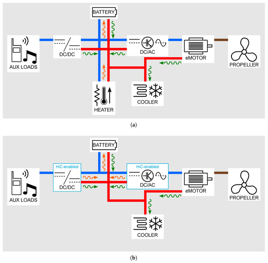
Figure 1.
Simplified diagrams for e-boat architectures: traditional approach based on a dedicated Joule heater (a) and innovative pseudo-cogeneration approach by Heater-in-Converter technology (b). The color of the interconnection denotes the type of energy transfer: blue for electric, red for thermal, and brown for mechanical. The wavy lines represent the heat flux: green for normal operation and orange for heating during cold start. The HiC-enabled components (highlighted in light blue) in subfigure (b) fulfill the heating function, thus allowing removal of the heater; it is not mandatory that all the converters are HiC-enabled. The heating flux to DC/DC, DC/AC, and motor is omitted for better clarity of the graphical representation.
HiC can modulate the power electronics converters (PECs) efficiency by specific Active Gate Drivers (AGDs) installed in place of the common ones; they drive the power components in a less efficient way by manipulating gate voltage or device current in a controlled fashion. This modification has a limited footprint on the cost and complexity of the system, and enables a plurality of useful techniques. For example, the adjustable loss can be used to reduce the thermal cycles amplitude undergone by the devices, thus improving their reliability, or to heat some system which needs specific climatic conditions, such as, indeed, batteries during cold start. The power loss which can be generated by HiC in addition to the nominal one of the PEC has an upper limit imposed by the safe operation of the whole converter: devices, boards, passive components, and chassis must remain below their critical temperatures. This temperature limitation becomes a power loss limitation in dependence of the specific properties of the thermal interfaces. In fact, PECs are constituted by layers of different materials (power device/module, heatsink, board, etc.), each of which exhibits a specific thermal resistance, i.e., a temperature difference per unit of power traversing the surface of heat exchange. Therefore, to design an effective HiC system, the thermal interfaces that are under system designer’s control (converter–liquid and liquid–battery) must be carefully designed, by choosing the most appropriate Thermal Interface Material (TIM); this allows achieving the target temperature change in the battery with minimum power loss, thus completely removing the need for a specific heater.
All this considered, to properly size the HiC-based heating system, it is required to determine its thermal load for the expected working region and the starting temperature distribution over the year. The difference between the target temperature of the battery and this distribution gives the distribution of the needed temperature variation over a time span of one year. This is important to limit potential overdesign arising from a worst-case sizing of the system. To accomplish this target, a model-based approach is used: a complete model of the environment where the target system works is given, starting from its latitude and few historical data about the local weather (transfer function from air to water temperature), to get distributions of air, water, and, ultimately, boat interior temperatures. The validation of this chain of models is done partly by using data available in public repositories and partly acquired directly on a test boat, docked near to Ravenna (Italy). To determine the required design power, the boat temperature distribution is matched with the maximum current (or power) vs. temperature–SoC function of the battery and with the typical time for the boat to reach the nominal speed and power. This information, coupled with a thermal model validated on the data coming from a reduced scale heating-and-cooling system, allows us to precisely determine the heating power requirement to guarantee the heating time, as a function of the thermal impedance of the coupling between the battery and its plates. The thermal test bench has a battery pack in 1:5 scale in terms of power and energy capacity, with respect to the typical powertrain of a seven meter long boat.
This study is pursued in the “PSEudo-COgeneration for Battery heating on electric and hybrid Boats” (PSECOB2) project. As it is funded by the Interreg ADRION initiative, most of the data presented in this work refer to the Adriatic-Ionian area of Italy as Figure 2 illustrates; Table 1 and Table 2 summarize the typical air and water temperatures of the studied cities (mean values of the year 1999–2019 period [23]). Nevertheless, the models provided were also partly validated in other locations and supply location-independent generalization of the proposed solution to other areas.
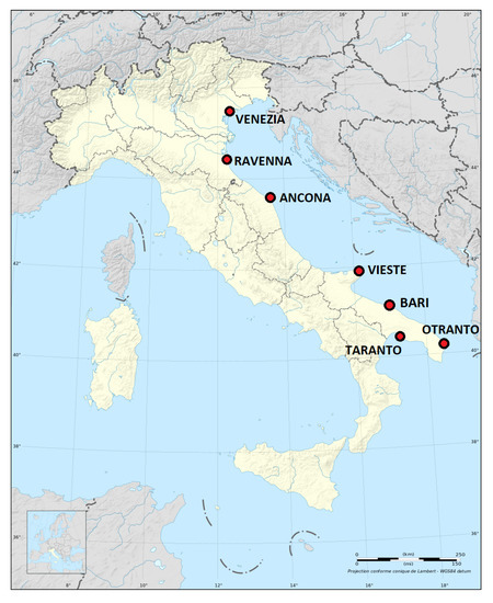

Table 1.
Typical air temperatures of ADRION cities (mean values of year 1999–2019 period [23]).
Table 2.
Typical sea water surface temperatures of ADRION cities (mean values of year 1999–2019 period [23]).
The following of this paper is structured to describe all the used models in Section 2, the results of which are reported in Section 3. The research outcomes are discussed and commented thoroughly in Section 4, and final conclusions are drawn in Section 5. Only the model for solar irradiance from latitude information is reported in Appendix A, as it has been part of the state-of-the-art for a long time and is presented just for clarity.
2. Materials and Methods
The core of this work is the model-based design process for the pseudo-cogenerative heating system to be used during the cold-start phase. The main aim is to minimize the required heating power, so that the whole heating stage is sustained by the HiC-equipped PECs on board. Several models are implemented and interconnected to reach this objective:
- Latitude to solar power model (LSPM), to determine the solar irradiance (i.e., the power per unit of area) received at the latitude of usual operation of the vehicle.
- Sun power to air temperature model (SPATM), to estimate the air temperature from the solar irradiance.
- Air temperature to water temperature model (ATWTM), to estimate the water temperature with respect to the air temperature.
- Boat temperature model (BTM), to forecast temperature distribution seen by the onboard battery.
- Battery limitation model (BLM), to identify the target working temperature for the battery, with respect to battery temperature and state of charge (SOC).
- Battery heating/cooling model (BHCM), to infer the required power from HiC technology, without the heater.
Their relationships are graphically represented in Figure 3. The validation and source data are gathered from different origins, depending on each specific model:
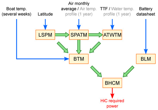
Figure 3.
Schematic representation of the information flow for the presented model-based design approach for HiC heating power: the interdependence of the models is shown. Blue denotes the input data needed (gray text for optional items), internal data is in green, and red is the final output of the process.
- LSPM: PhotoVoltaic Geographical Information System (PVGIS) simulator [25], developed by the European Joint Research Center and available at its official website [26], open-access.
- SPATM and ATWTM: Italian National Tide Gauge Network of ISPRA (Institute for Environment Protection and Research, provider of the European Joint Research Centre) [23], open-access, and Daphne unit of Agenzia Regionale per la Prevenzione, l’Ambiente e l’Energia of Emilia-Romagna region (ARPAE) [27], available on request.
- BTM: Data collected directly by the authors on a test boat docked near to Ravenna harbor.
- BLM: Datasheet provided by the cell manufacturer.
- BHCM: Data collected directly by the authors on the 1:5 reduced-scale test bench for battery heating/cooling system.
It must be noted that the major concern for the model chain presented here is not to get an accurate meteorological-grade temperature forecast, but to determine the boat temperature distribution over an entire year. By definition, this information is uncertain: it depends heavily on the type of boat, specific atmospheric conditions, travels undergone during the year, type of berthing, etc. Moreover, looking at the yearly distribution rather than at the worst case allows understanding the impact of a power limitation in statistical terms: using worst-case temperature difference may lead to system over-design if this condition happens rarely over the year (or the period of interest). This is the reason why, for example, the simple Kepler model can be used to implement LSPM in place of more complex ones [28]. Each model is detailed in the following sections, with the sole exception of LSPM, which is directly taken from literature and reported, for clarity, in Appendix A.
2.1. Sun Power to Air Temperature Model
At large scale, the air of open environments has complex thermal interactions with the incoming solar irradiation and the surroundings (see, for example, in [29,30,31]); in addition, many variable effects (such as wind, rain, and cloudiness) should be taken into account to get an accurate dynamic representation. However, as we are interested in overall annual trends, we are able to model air temperature in a simpler way. It is known that monthly average air temperature correlates with average Sun irradiation, as long as we consider a one-month lag between the two quantities [32]. Therefore, it is possible to develop a linear model which takes into account only solar irradiation S (collected from datasets or computed with LSPM, see in Appendix A), elevation of the studied point from the ground E, and the “lapse rate” of temperature loss along elevation L [32]. In particular, adapting the model provided there to coastal regions (it was originally designed for mountains), it is possible to predict the average air temperature of month by the relation
which fits , , and coefficients using empirical data and a least-square procedure.
To reconstruct the water temperature, the power from LSPM is integrated over time, to get the monthly average Sun irradiation, then the work in (1) is applied, yielding the monthly average air temperature. The resulting points are thus interpolated with a yearly frequency sinusoid, thus getting a daily-average information. It can be observed that the amplitude of the daily oscillation of air temperature is fairly constant over the year and it depends on the considered location only (see in Section 3.3); this component, obtained from the frequency analysis of the real temperature data, is added to the aforementioned sinusoidal yearly fit. The final result is a two-harmonic (plus offset) reconstructed air temperature trend, including both annual and daily dynamics, which is the valuable input for the following model. This follows both the commonsense and the experimental evidence: air temperature has a periodic waveform mostly due to the revolution of the Earth around the Sun; possibly, it also contains higher order harmonics, connected to the daily rotation.
2.2. Air Temperature to Water Temperature Model
This model estimates the annual trend of sea surface water temperature of a selected coastal city, given the environment air temperature of the same location (collected on datasets or computed with SPATM). The implementation is done by analyzing the data (ISPRA and ARPAE sources) in the frequency domain, by means of Fourier transform. More appropriately, as all datasets are time-sampled (possibly with a one-hour time base), the Discrete Fourier Transform (DFT) is used:
Following the simplifying assumption that the water temperature is determined mainly by the temperature of the air mass above it, it is possible to compute the so-called “Thermal Transfer Function” (TTF) as the ratio between the two DFTs of temperatures:
According to this approach, the air temperature entirely determines the water temperature, considering all the location specific parameters (orography, shore shape and orientation, water reservoirs nearby, etc.). Despite its simplicity, this idea is supported by the data, as it can be noticed in Section 3.3: computing the TTF for many years, it stays constant, while differing slightly among locations. At last, we can apply the proper location environment transfer function (3) to predict the annual trend of water temperature. We end up with an annual set of Sun radiation, air temperature, and sea water temperature to be used for the internal boat temperature modeling.
To validate this model, seven Italian cities in the ADRION region have been studied: Ancona, Bari, Otranto, Ravenna, Taranto, Venezia, and Vieste (see in Figure 2). For each of them, the collected air and water temperature datasets are relative to the 1999/2019 period and have been sampled hourly. All data were subjected to a preprocessing phase, resulting in a database formed by a dozen datasets per city, each of them having 8760 samples. The preprocessing consisted in
- removal of extra data relative to leap years;
- selection of datasets having more than 90% of yearly data and less than 0.5% of outliers in them;
- linear filling of missing data;
- outlier replacement by the means of a moving median method, computed on a window of 24 samples (one day); and
- matching of the air and water datasets which both satisfied the selection process.
2.3. Boat Temperature Model
To relate the internal boat temperature to the external environment quantities (Sun irradiation, air temperature, and sea surface water temperature), we sampled the actual internal temperature of a typical pleasure boat (Janneau Cap-Camarat 5.5 WA) moored at Porto Garibaldi (Ravenna, Italy) for about three months (71 days, from 14 June 2020 to 23 August 2020, corresponding to the mooring period of the boat under test). This period, spanning three months, is the longest period that was compatible with the travel restrictions imposed in Italy due to COVID-19 outbreak. Data were collected continuously, using the unmanned Temperature-Humidity Datalogger RS-172TK. Comparing this data with the local air and water temperatures (see in Section 3.4, Ravenna values used), we noted that the mean boat temperature is strongly dependent on the water one, while its ripple is attributable to air and sun radiation, which both possess a characteristic daily dynamics. The Sun power was considered as the internal temperature of the boat can rise above the outside one: this can be ascribed to small-scale greenhouse effect, thus determined by the direct radiation received.
It is thus possible to perform a multivariate regression (least-square) of the internal temperature , using air temperature , water temperature , and Sun irradiance as predictors:
To support this procedure, we also trained a Support Vector Machine (SVM) learning algorithm [33] to infer a model with the same structure as (4). SVMs are a wide group of supervised learning algorithms used for classification and regression problems. They can enhance traditional regression algorithms by adding some slack hyperparameters which are then minimized by convex optimization schemes; in particular, we used the linear epsilon-insensitive regression loss function implementation of SVM [34,35]. Given the short time span covered by the directly-collected boat temperature profile (see in Section 3.4), the validation of the model is obtained by splitting the dataset in two chunks, covering 80% and 20%, respectively. The first chunk is used to fit the data (training), while the latter provides the population for the validation (test).
Following the chain constituted by LSPM, SPATM, ATWTM, and BTM, it is possible to estimate the internal boat temperature for any day of the year, given the design location coordinates and an annual chart of its environmental air temperature, combined with the TTF: this information allows determining the heat load of the Heater-in-Converter system.
2.4. Battery Limitation Model
To determine the heat load required for the Heater-in-Converter system, the target working point temperature for the battery must be known, as well as the time span available to reach it. The latter depends on the type of boat and the typical activities going in and out of the port, while the former depends on the cell model and chemistry. The information about is best retrieved from the cell datasheet, where a typical maximum current vs. cell temperature and state of charge table is given . Multiplying this for the relationship the safe-managed power is obtained. The main problem of this procedure is usually the poor resolution of the data. This can be overcome by higher-than-linear 2D interpolation; using a cubic algorithm is a good solution.
From the specific application (vehicle, boat, type of driver, etc.) a requirement of worst-case is available: the curve is thus projected for , with solution , where is the application-dependent power which the vehicle designer wants to guarantee to the driver in . The battery cells discharge current map is illustrated in Figure 4a, together with its cubic interpolation on a finer grid (Figure 4b).
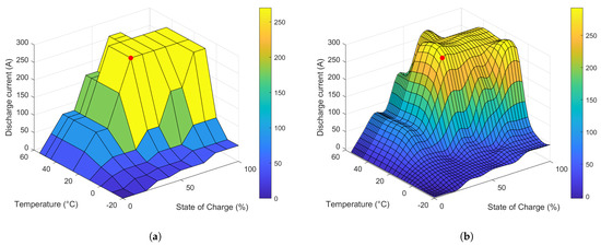
Figure 4.
Battery discharge current map of a typical commercial LFP cell (EVE LF90), expressed as a function of temperature and state of charge (a), and its finer interpolation (b). The target design point (25 °C, 270 A, 50% charge) is shown as a red dot.
2.5. Battery Heating/Cooling Model
The main objective for HiC is to enable battery heating at cold start without adding significant volume, cost, and weight to the system, while removing the specialized heater. In this view, the heating system shares the thermal circuit with the cooling one: as long as the components are below their rated temperature, the heating action is used, while the cooling functionality is actuated in all other conditions. This model is used to estimate the thermal load of the HiC, starting from the knowledge of the surrounding boat environment temperature (BTM) and of the target battery working point (BLM).
The general thermal fluid circuit of the boat battery heating/cooling system is given in the schematic representation in Figure 5. It is constituted by the following components: pump, fluid cooling device, fluid heating device, battery, and battery heating/cooling device. The pump is needed to provide constant mass flow through the circuit. A fluid cooling device is required to chill the thermal fluid, and it prevents the battery from overheating in duty conditions. The fluid heating device is the core component of the studied circuit: it is responsible for the fast heating transient of the battery, from cold start to operative conditions; in modern systems, it consists of a resistive heater, while in the authors’ proposal it is the pseudo-cogenerative DC–DC converter. Other converters can be used as well (such as the traction inverters, provided that they are equipped with HiC technology at the circuit design stage). The battery plates are in charge of both battery heating, in cold-start situation, and battery cooling, in duty conditions. A reduced-scale test-bench of this system was developed within the PSECOB2 project; it is reported in Figure 6. It implements a centrifugal pump for thermal fluid circulation, a fan radiator for fluid cooling, a dedicated resistive heater (to compare HiC to standard technology), the DC–DC pseudo-cogenerative converter (heatsink only in figure) and three heat-exchange plates, responsible for battery heating and cooling. Sheets of TIM are interposed between each battery plate and cells; there are also two diverter valves, which allow bypassing the resistive heater when needed. The component specifications are listed in Table 3. In addition, the battery pack is equipped with three Type-J thermocouples and the water circuit with a flow meter and five Pt100 resistance temperature detectors (RTDs). To size the battery pack, we considered that the motor installed on typical small (5 to 6 ) pleasure boat usually has a rated power of about 100 and a capacity of 25 to 35 . To simplify the implementation of the test bench, we developed a 1:5 down-scaled version of the system (both in power and capacity). Eventually, once the model is properly validated, we may scale up the simulation and test the performance on different and bigger battery sizes. The scaled battery power of 20 – 8 was achieved in our test bench by connecting in series 28 commercial LFP 90 capacity cells, rated at discharge current.
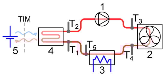
Figure 5.
Thermal schematic of the heating/cooling system of the battery: pump (1), fan cooler (2), one ore more electric heaters (3), battery heat-exchange plates (4), and battery pack (5). T1–T5 are resistance temperature detector (RTD) sensors to measure the fluid temperature, while the battery temperature is sensed by three thermocouples.
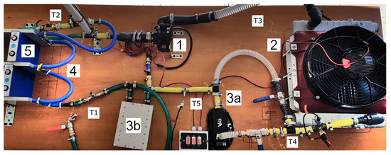
Figure 6.
Test bench implemented for heating/cooling system model validation (see in Figure 5). We note the pump (1), the fan radiator (2), the resistive heater (3a), the DC–DC converter heat plate (3b), the battery heat-exchange plates (4), the battery (5), and five temperature RTD sensors (T1–T5). Two diverter valves allow to bypass the resistive heater, if desired.
Table 3.
Test bench components specifications.
The simulation model of the heating system was designed using Mathworks Simulink® and Simscape™ to match the simulated component parameters to their test bench representatives. The pump is modeled as an ideal constant mass flow source and keeps circulating the heat transfer fluid (which is assumed to be pure water, ) at the measured rate. The fluid cooling component, representing the fan radiator, is modeled as a heat flow source that extracts heat based on a datasheet-tabulated thermal resistance curve. The fluid heater (used for the model calibration) is modeled as a constant heat flow source of 2500 (the nominal value of the traditional heater installed in the bench). The battery pack, which completes the circuit, is represented by two thermal capacities and is affected by the heat transfer coming from the adjacent plates, modeled as three constant-temperature source components. It is important to note that the battery was not active during the test bench experiments, so we neglected its Joule heating contribution in the validation of the model.
The overall LiFePO4 battery specific heat capacity is expected to be comprised in the range 825 to 1360 [36,37,38,39,40]; in our particular case, the manufacturer declared , which is the adopted value. One last crucial aspect to be considered is the temperature drop due to the imperfect contact among the battery and the plates: the TIM is modeled by the addition of a consistent thermal resistance (contact resistance). However, the direct measurement of this quantity is quite difficult and would require complex instrumentation [41,42,43,44]: interface surface roughness, objects materials, and contact pressure are only three of the principal factors determining this parameter [45,46,47,48]. We can therefore calibrate the thermal contact resistance to match the test bench measurements and then generalize the results to other sizes of the bench.
3. Results
3.1. Latitude to Solar Power Model
LSPM implementation (Appendix A) is validated by comparing its results with the data collected from PVGIS [26]. As the model results strictly depend on the studied location, several cities of the world have been tested. However, solar irradiation is not related to longitude (due to Earth rotation during a day) [49]: therefore, we evaluated the model behavior at different places located at different latitudes, but with similar longitude. In particular, Figure 7 and Table 4 illustrate the validation of LSPM for the ADRION region, while Figure 8 and Table 5 focus on some other major cities of the world distributed along the same meridian. Incidentally, it is worth noting that both Kepler’s method and direct ODE solving were tested and provided indistinguishable results.
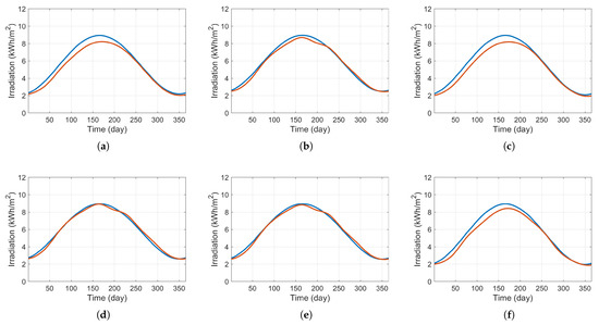
Figure 7.
Comparison of daily average clear-sky irradiation computed with LSPM (blue) and retrieved from PVGIS (red) in the ADRION cities: Ancona (a), Bari (b), Ravenna (c), Otranto (d), Taranto (e), and Venezia (f). Substantial superposition of the two curves is appreciable for all of them (see Table 4 for numerical validation). As expected for northern hemisphere locations, the highest values of irradiation are registered in the central part of the year.
Table 4.
RMSE, normalized on the mean value, of LSPM with respect to PVGIS data in ADRION region (see in Figure 7). Negligible error is observable.
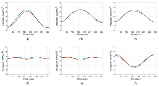
Figure 8.
Comparison of daily average clear-sky irradiation computed with LSPM (blue) and retrieved from PVGIS (red). Some of the major cities of the world belonging to the ADRION meridian are considered: Berlin (a), Tazouta (b), Khourigba (c), Libreville (d), Kinshasa (e), and Capetown (f). Substantial superposition of the two curves is appreciable for all of them (see Table 5 for numerical validation). It is notable that the peak of irradiation shifts through the year in function of latitude. Cities near the equator manifest a nearly-constant irradiation trend over time.
Table 5.
RMSE, normalized on the mean value, of LSPM with respect to PVGIS data outside ADRION region (see in Figure 8). Negligible error is observable.
3.2. Sun Power to Air Temperature Model
Table 6 summarizes the results, and Figure 9 shows the comparison between the model and the historical data from the ISPRA database. In these figures, one city (Vieste) was omitted to give a better visual layout; its results are in line with those of the other cities. To validate this procedure, we compared (1), calibrated on the first year of the data set, to all other years of sampled data: we observed that the calibrated coefficients consistently represent each location air temperature trend through time. Table 6 reports the global RMSE of the model, i.e., computed on all years, using the coefficients determined on the first year only available in the data set of each town.
Table 6.
Monthly-average air temperature model coefficients calibrated on the first year available for each city, and RMSE error computed on all sampled years, with reference to model (1).
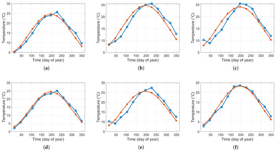
Figure 9.
Comparison between ISPRA monthly-averaged air temperature, in blue, and its reconstruction using the calibrated model (1), in red. Substantial accordance of modeled trend to sampled data is observable (see Table 6 for numerical data). Cities shown: Ancona (a), Bari (b), Otranto (c), Ravenna (d), Taranto (e), and Venezia (f).
Figure 10 reports the annual average of daily air temperature oscillation amplitude; it is shown that this quantity is almost constant over 18 years. Figure 11 compares the historical dataset of one year for each city with respect to the air annual temperature profile as reconstructed by the SPATM.
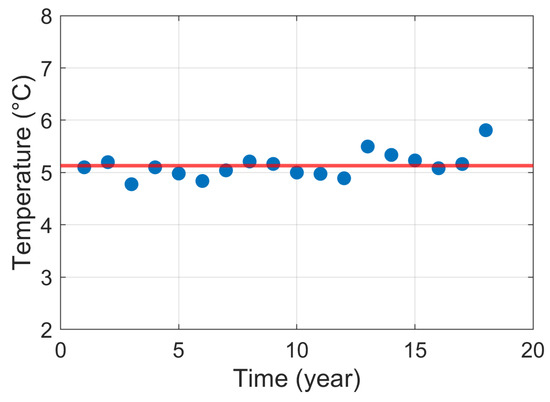
Figure 10.
Annual average of daily air temperature oscillation amplitude (blue dots) and global city mean (red line); stationary trend is observable. Example shown for Ancona, for all the sampled years.
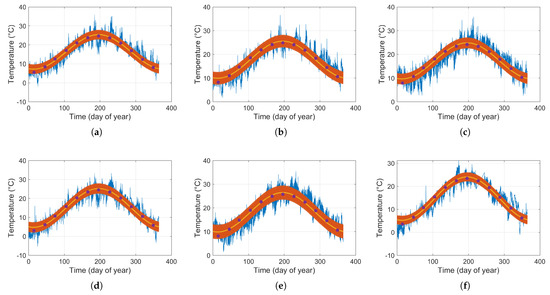
Figure 11.
Air temperature reconstruction: original ISPRA data (blue), monthly average reconstruction computed with model (1) (purple), yearly sinusoidal fit of monthly average (yellow), complete air two-harmonic reconstruction with the addition of modeled daily trend (red). Cities shown: Ancona (a), Bari (b), Otranto (c), Ravenna (d), Taranto (e), and Venezia (f).
3.3. Air Temperature to Water Temperature Model
The spectral analysis of air and water temperatures shows that there are three major harmonic components; in descending amplitude order: the average value, a yearly harmonic, and a daily harmonic. These components match the two main expected motion cycles of Earth around the Sun: yearly revolution and daily rotation [50]; Figure 12 illustrates an example of air and water temperature spectra. It is noticeable that water possesses a very weak daily spectral component, due to its expected high thermal capacity; Figure 13 clarifies this concept, showing a comparison between the original air and water temperatures profiles and a simplified reconstruction based on the two-harmonic model. The time shift between the air and water temperature is noticeable; it can be ascribed to the equivalent high thermal capacity of the sea water itself [51].
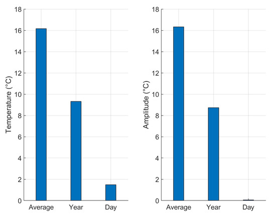
Figure 12.
Example of Ancona air (left) and water (right) temperature Fourier Transform harmonic amplitudes, year 2000. Three main components are present, in decreasing order: average value, yearly component (due to Earth revolution around the Sun), and daily component (due to Earth rotation). It is observable that water manifests a weaker daily component because of its higher thermal capacity.
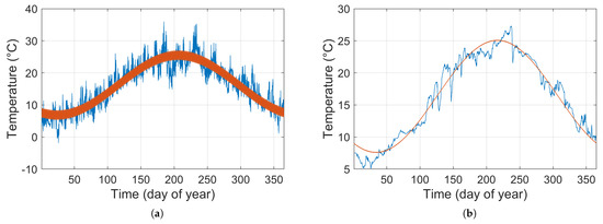
Figure 13.
Comparison of Ancona air (a) and water (b) sampled temperature (blue) with their respective 2-harmonic model (red) (year 2000).
Figure 14 represents the three main components of the TTF for all the sampled years of our database; each city presents constant values over time: this means that though the environmental temperature transfer function is characteristic of a specific location, it is not a function of time. Comparing the values for various cities, we note that the ADRION region manifests a fairly consistent behavior, therefore we can characterize the overall ADRION TTF as the average of each city contribution. Table 7 summarizes the aforementioned results.
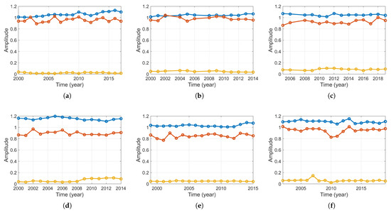
Figure 14.
Temperature transfer function amplitude values at the main spectral components, for each ADRION studied city: average component (blue), yearly component (red), daily component (yellow). Cities shown: Ancona (a), Bari (b), Otranto (c), Ravenna (d), Taranto (e), and Venezia (f). It is notable that the spectral components are mainly constant over time for a given location and only change in dependence of the studied place.
Table 7.
Environmental temperature transfer function amplitude components and relative normalized standard deviation error. All quantities are dimensionless, as they descend from the ratio of two temperature DFTs.
3.4. Boat Temperature Model
Figure 15 shows a comparison between the 2020 Ravenna air and water temperatures retrieved from the ISPRA database and the experimental sampled boat internal temperature, in the same period of time. Detailed information about internal boat temperature is not available in literature, therefore a measurement campaign was undertaken to collect such data. By fitting the model (4) to these data, a relationship to extrapolate the results to all the year is identified; the boat model parameters are summarized in Table 8. Figure 16 offers at a glance the performance of the BTM. As two extrapolation methods are used (least-square fitting and SVM fitting), two model curves are reported there (green and purple). The two methods of extrapolation give consistent responses, so it is safe to compute the boat temperature extrapolation through the simpler least-square regression approach.
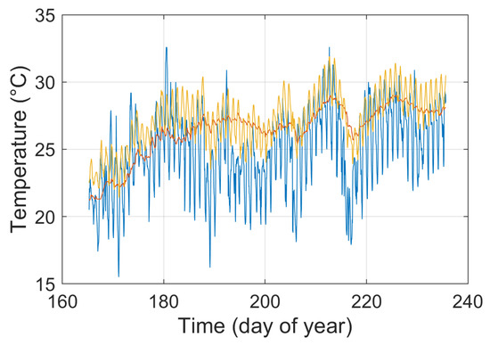
Figure 15.
Sampled boat internal temperature (yellow) compared with Ravenna air (blue) and water (red) temperatures [23] between 14 June 2020 and 23 August 2020. The boat trend is notably influenced by water temperature.
Table 8.
Internal boat temperature extrapolation coefficients information. These results pertain to 1689 observations and score at RMSE = , .
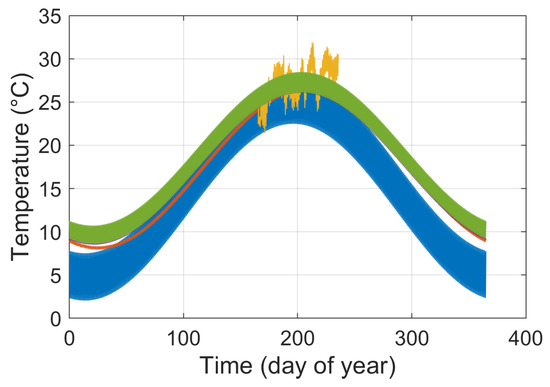
Figure 16.
Extrapolation throughout the year of the sampled internal boat temperature (yellow), with respect to Ravenna air temperature (blue) and water temperature (red); the extrapolation model outputs are included: least-square extrapolation (purple) and SVM algorithm extrapolation (green). The yellow trace pertains to the data of Figure 15 and spans over a limited fraction of the year, corresponding to the maximum extension of the experimental data set which was acquired. Note that the purple line is almost completely hidden by the green one.
3.5. Battery Heating/Cooling Model
Measurements on the 1:5 test bench for the heating system showed that, in stationary conditions, a water flow of traverses the circuit: using the resistive heater at full nominal power ( 2500 ) for about 15 min, we initially obtained the temperature increases reported in Table 9. Following a trial-and-error process, it is possible to tune the thermal resistance between the plates and battery: Figure 17 presents a comparison between some sampled test bench temperature trends and the corresponding modeled ones, with . This value, obtained without the TIM installed (i.e., putting plates and battery in direct contact and adding pressure), is far too high; therefore, we applied the TIM identified in Table 3, with a declared of of the previous one.
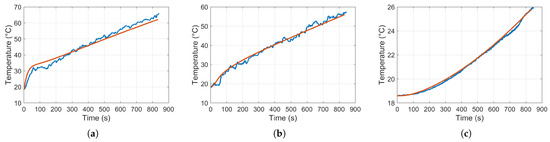
Figure 17.
Validation of the heating system model. Comparison between test bench (blue) and simulated temperatures (red), with respect to Figure 6 points: T5 (a), T2 (b), and battery (c).
3.6. Overall System Design Outcomes
Once the boat model is validated and the heating system one is tuned based on the TIM thermal resistance, they can be applied for the effective battery heating/cooling system design. The time needed for a real departure from mooring was measured by GPS tracking on the test boat docked near to Ravenna (see Figure 18): it resulted in 17 min, so . As the extrapolation model for the boat temperature exhibits a plateau at 10 between days 0 and 50, i.e., for roughly 14% of the year (see Figure 16), this is assumed to be the relevant design value for . Following the choice made in Figure 4, the target battery temperature is set to . The heating system is therefore required to produce a net temperature increase of within the estimated . It is important to note that, as pointed out by the blue curve in Figure 16, sizing the system on the air temperature worst case would highly oversize the HiC system, resulting in a minimum of 3 , thus resulting in a required temperature step 46% higher than the proposed one.
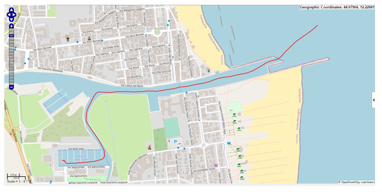
Figure 18.
Sampled GPS track of test boat departure from Porto Garibaldi dock (Ravenna, Italy). Starting coordinates at 05:12 AM: [44.67 N, 12.23 E]. Ending coordinates at 05:29 AM: [44.68 N, 12.25 E].
To study this scenario, we scale up the thermal capacities of BHCM by a factor of five, to compensate for the scale of the system [52]. However, we realized that the heating system was not able to achieve the target with as it was: the high thermal contact resistance between battery and plates, modeled upon the test bench coupling, would cause an excessive heating device sizing, due to the excess drop between the plate and the cells. Therefore, a highly conductive thermal interface material, installed with an adequate contact pressure, is mandatory for proper sizing of the HiC-based system. By leveraging the model-based nature of the simulation, we explored different scenarios of thermal coupling and heating power inputs: Figure 19 illustrates the simulated heating time as a function of these two quantities. By imposing the target time and by fitting the simulated working points, it is possible to express the heating power as a function of thermal contact resistance: the adopted simple linear model (see in Figure 20) can be expressed through the relation
where and are the fitting parameters, is the HiC target power (in ), and the thermal contact resistance (in ). By choosing a Shariag NF-150 silicone thermal pad and an overall battery area of , a resistance of is obtained. Therefore, we adopted this TIM and chose the final design power for the HiC converter for the target boat to be 6 .
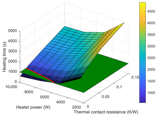
Figure 19.
Simulated heating time as a function of battery-plates thermal contact resistance and heater power. The target heating time is represented as a green plane while the red line illustrates the minimal power curve for system sizing. Data refer to full-size system, not to the test bench.
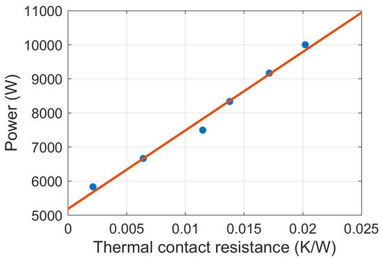
Figure 20.
Heater power in function of battery–plate thermal contact resistance, for a heating time of and for the full scale system. Simulated scenarios shown as blue dots, fitted model as red line.
4. Discussion
Looking at Section 3, it is clear that the model-based design approach to HiC converters for battery heating is rather complex, yet the model chain has been validated and the final additive power requested by the HiC converter for a 100 boat powertrain is identified in 6 .
Section 3.1 demonstrates that the planetary model is accurate enough to provide the clear-sky sun irradiance, even in instantaneous terms, as denoted by the superposition of this model (regardless of the specific implementation) with the data collected by the PVGIS repository. Therefore, no specific data are required at this stage: just the location latitude value or interval is needed. Considering the clear-sky irradiance rather than the direct normal irradiance may seem a coarse approximation, but the consistency of the subsequent models, entirely based on “clear-sky” rather than “direct normal”, suggests that more complex models (such as those in [28]) are not needed.
Indeed, the Huang approach on inferring air temperature from solar irradiation [32] is more troublesome, as denoted by Figure 9. Considering that, in the best case, SPATM requires tuning on the monthly-average data, there is a trade-off between accuracy and cost of retrieving information: the hourly profile of air may be unavailable, especially in certain places, conditions in which the SPATM approach ensures a simple solution. In addition, if daily data are available, using it for the design leads to improved accuracy. The stable profile of annual-average daily air temperature oscillation amplitude depicted in Figure 10 suggests that data from a single year only can be considered, thus suggesting also that collecting many years can be an excessive effort for this application. Nonetheless, the comparison of data and SPATM in Figure 11 proves that our model provides a reasonable accuracy while also giving a daily ripple figure.
Figure 12 and Figure 13 confirm what commonsense suggests: the steady-state behavior of both air and water temperatures is highly connected to the Sun power as resulting from yearly revolution and daily rotation: frequency analysis is absolutely the right tool to face the problem. For the other frequency components, the analysis showed that they are not periodic, as noticeable, especially for water, in Figure 13. Figure 14 and Table 7 provide a very strong result: it is possible to find a TTF typical for each location, often characterized by very small coefficients for the daily component, which is almost absent from the water while being relevant for the air. The similar values of TTF of the different ADRION cities considered point out the possibility to determine the TTF also in locations slightly far away from the desired one, without excessively losing accuracy. It is still unclear to the writers the reason why the average temperature of water is slightly higher than the one of air. Possibly, some radiative dispersion of air during the night is involved [53].
Concerning internal boat temperature yearly profile estimation, Figure 16 and Table 8 ratify that the proposed linear model is satisfactory, regardless of the fitting done using traditional least-square procedures or more modern SVM-based techniques. A remarkable outcome of Figure 15 is the massive effect of water temperature in determining the boat one, and the need to consider a reasonable ripple caused mainly by Sun irradiation and small-scale greenhouse effect inside the boat.
Despite the relevance of the models discussed above, the core of the design effort is sustained by BLM and BHCM. While the battery limitation issue can be solved by datasheet-available information, the uncertainty in the of the TIM between battery plates and the cells of the pack requires a non-trivial calibration procedure [54], which we were able to complete thanks to the reduced-scale test bench. The comparison in Figure 17 confirms the correctness of the lumped BHCM model and its accuracy once the TIM is properly accounted for. The paramount relevance of the TIM properties in the sizing of the HiC heater and in the performance of the heating/cooling system is reaffirmed by Figure 19 and Figure 20. Despite the system being nonlinear, the experimental evidence shows that if a constant is considered, the relationship between TIM thermal resistance and required heater power is almost linear.
It is clear that each of the presented models is an essential element to cope with the initial problem, i.e., the sizing of the heater for e-boat batteries. Each model plays a key role in gathering all the relevant information from the environment (irradiance, air and water temperatures, etc.) and pertaining to component properties (boat shape and materials, heating/cooling system, etc.). Even if the proposed model chain is quite long, it develops almost linearly; overall, the key objective for this analysis is achieved: providing the system and power electronic designers the requirements for the HiC heater and for the materials (i.e., the TIM layer and the liquid circuit dimension) influencing them most. This approach is mandatory as working simplistically on worst-case (coldest) air temperatures from weather datasets yields unnecessary system over-design.
This study calls for the use of a 6 heater in a 100 powertrain. This value represents a theoretical efficiency of 6%, but the nominal heat must occur at low loads, resulting in a much lower target efficiency in case of HiC. The technology, currently at TRL 4 and targeting TRL 6 by the end of the PSECOB2 project, still presents open points about the minimum achievable efficiency (therefore, maximum heating power): the exact quantification of this aspect is still uncertain and requires further investigation, because of its impact on converter reliability [55]. Nonetheless, it is reasonable to argue that higher heating power levels can be achieved by converters with higher ratings. Despite this possible technical limitation, the HiC technology is fully viable from the economic point of view: adopting AGDs to enable HiC functionality in the converter requires combined design and component costs in the range of 7 to 15 USD per part (almost independent from the heat target), with a batch of one thousand units. Thus, HiC can compete with heaters in the 100–300 USD band. In addition, HiC technology can be applied fruitfully also to other full-electric vehicles: we proposed a marine environment, but no element is expected to be exposed to the salty and windy aggression typical of this environment. What is really needed to adopt this technology is the availability of an onboard PEC with a sufficient power rating to accommodate also for the temporary lower efficiency request by HiC.
5. Conclusions
We presented a chain of models to generalize the determination of inner yearly boat temperature distribution, relying on the knowledge of the target location coordinates and a yearly dataset of its environmental air temperature. We developed a simplified model to predict the average solar radiation in any day of the year. Thanks to this information, we reconstructed the yearly trend of air temperature, including its typical daily oscillation. Then, the link between environmental air and surface water temperature was investigated: we observed that both temperature profiles could be easily described by the sum of three harmonics (DC, year, and day). The transfer function between the two quantities has proven to be constant over time and dependent only on the considered location: leveraging this fact, we could retrieve the yearly trend of water temperature through its modeled transfer function. Next, we studied the relationship between the set of the three aforementioned external quantities (solar radiation, air temperature, and water temperature) and the internal temperature of a boat, eventually getting to a simplified multilinear model. This model was validated on data collected in the summer season; validating the extrapolation model in other seasons will also strengthen the proposed approach. The daily average boat temperature is mainly determined by the water one, but with an important fluctuation due to sun irradiance.
This process, yielding the boat temperature distribution over an entire year, allows not only considering a specific scenario (i.e., the lowest winter temperature or, much better, the distribution of the coldest months), but also estimating the impact of a reduced thermal power. This model also prevents overdesign of HiC heating, as it would result using the worst-case air temperature rather than the presented approach: simulations showed that a difference in excess of 40% is otherwise achieved. Knowing the optimal battery working point and the typical departure maneuver time, we were able to design a suitable HiC-based heating system. Finally, with the help of the PSECOB2 test bench, we validated the simulation: scaling its parameters, we can generalize the results to different boat battery sizes and different locations or period of the year. The TIM properties were revealed to be the key parameters for an effective HiC design. The value identified ( 6 ) will be used as the design requirement of the maximum power loss to be achieved by the HiC-enabled converter of the proposed application. The effectiveness of the scaled design will be validated in the bench, with an HiC power of , as heating power does not scale linearly with the system size.
The design of a fully HiC-based battery heating system, to be compared with traditional heaters, is an essential step towards an increased maturity of the technology: leveraging the presented model, a real system will be developed and evaluated, clarifying the production costs more in detail (possibly narrowing the current 7–15 USD band), and leading to deeper understanding of the heat power limitations. These factors are crucial for the applicability of Heater-in-Converter on many scenarios, especially those characterized by high heating power demand, in excess of 10 .
6. Patents
The battery heating system described in this work resulted in a pending Italian patent application, under the ownership of University of Parma.
Author Contributions
Conceptualization, D.F. and A.S.; methodology, D.F., A.S., and P.P.; software, D.F.; validation, D.F., A.S., and P.P.; formal analysis, D.F.; investigation, D.L. and P.P.; resources, D.L. and P.S.; data curation, D.F.; writing—original draft preparation, D.F.; writing—review and editing, all; visualization, D.F.; supervision, A.S.; project administration, A.S.; funding acquisition, A.S and P.P. All authors have read and agreed to the published version of the manuscript.
Funding
This research was funded by Interreg ADRION grant number 77_OISAIR project, innovation vouchers. The APC was funded by 4e-consulting s.r.l., Ferrara, Italy.
Institutional Review Board Statement
Not applicable.
Informed Consent Statement
Not applicable.
Data Availability Statement
Not applicable.
Acknowledgments
The authors warmly thank Matteo Dalboni for his kind support in proofreading the document and in improving the appearance of the bibliography.
Conflicts of Interest
The authors declare no conflict of interest. The funders had no role in the design of the study; in the collection, analyses, or interpretation of data; in the writing of the manuscript; or in the decision to publish the results.
Abbreviations
The following abbreviations are used in this manuscript:
| ADRION | Adriatic-Ionian area |
| AGD | Active Gate Driver |
| ARPAE | Agenzia Regionale per la Prevenzione, l’Ambiente e l’Energia |
| (Regional Agency for Prevention, Environment and Energy) | |
| ATWTM | Air Temperature to Water Temperature Model |
| BHCM | Battery Heating/Cooling Model |
| BLM | Battery Limitation Model |
| BTM | Boat Temperature Model |
| DFT | Discrete Fourier Transform |
| HiC | Heater-in-Converter |
| ICE | Internal Combustion Engine |
| ISPRA | Istituto Superiore per la Protezione e la Ricerca Ambientale |
| (Institute for Environment Protection and Research) | |
| LSPM | Latitude to Sun Power Model |
| PEC | Power Electronics Converter |
| PSECOB2 | PSEudo-COgeneration for Battery heating on electric and hybrid Boats |
| RTD | Resistance Temperature Detector |
| SOC | State of Charge |
| SPATM | Sun Power to Air Temperature Model |
| SVM | Support Vector Machine |
| TIM | Thermal Interface Material |
| TRL | Technology Readiness Level |
| TTF | Thermal Transfer Function |
Appendix A. Latitude to Sun Power Model (LSPM)
This model provides the clear-sky sun irradiance starting from the latitude of any location. “Clear sky” denotes that the effects of scattering and absorption due to clouds are neglected, while the absorption by the atmosphere is considered by proper derating of the solar constant. In fact, the solar irradiance that reaches the top of Earth’s atmosphere on a perpendicular plane to the rays is known as solar constant, and its value is 1361 / [56]. However, the interaction with Earth’s atmosphere gaseous components (O3, CO2, and O2) and water vapor contained in clouds [57,58] significantly reduces the irradiance received at ground: the effective value, used in many application fields, is estimated to be 1000 / [59].
To suit the use needs, this model must provide not only the Earth’s orbit, but also the position of our planet over time, connected with the start of the calendar year. The basic dynamic equation, assuming that the Sun is placed in the origin of the reference system, M is Sun mass, G the Universal Gravitation Constant, is the vector identifying the position of Earth with respect to the Sun, with X axis pointing to perihelion and Y axis perpendicular, radians apart, turning counterclockwise, is (dot denoting the time derivative)
Equation (A1) is a nonlinear system of two second-order ODEs; it can be solved numerically by common tools [60], provided that the initial position and speed are known. These are determined starting from the revolution period and the orbit eccentricity e, defining :
A simpler solution to this problem was found by Kepler back in 1619, leading to the formulation of Kepler’s laws and his system of anomalies [61]. The mean anomaly is a function of time t representing the angle of the planet if it moved on a circular orbit; the eccentric anomaly is obtained by solving the transcendental equation
The true anomaly (angular position of the planet) is
Ultimately, the distance between Earth and Sun is given by
where a is the orbit maximum semiaxis.
Once the Earth orbit is determined in space and time by using (A1)–(A3) or (A4)–(A6), the position of the Sun in the local reference frame (studied location) placed at a given geographical point is obtained by composing the rotation matrices
where S is the frame centered at Earth’s center of gravity and oriented as the ecliptic plane, T is the frame moving with Earth and oriented as its tilt angle (about 23.5°) with respect to the ecliptic plane, O is the frame of an observer located on Earth’s surface, and C is the same frame re-oriented by a compass indication (i.e., with x to East, y to North, and z to Zenith). The power is therefore obtained by dot multiplying this position by the vector indicating the direction the surface receiving the light is oriented to (horizontal for the sea).
References
- European Commission. Green Airports and Ports as Multimodal Hubs for Sustainable and Smart Mobility; Call ID: LC-GD-5-1-2020; 2020. Available online: https://ec.europa.eu/info/funding-tenders/opportunities/portal/screen/opportunities/topic-details/lc-gd-5-1-2020 (accessed on 1 February 2021).
- Sciberras, E.A.; Zahawi, B.; Atkinson, D.J.; Breijs, A.; van Vugt, J.H. Managing Shipboard Energy: A Stochastic Approach Special Issue on Marine Systems Electrification. IEEE Trans. Transp. Electrif. 2016, 2, 538–546. [Google Scholar] [CrossRef]
- Gennitsaris, S.G.; Kanellos, F.D. Emission-Aware and Cost-Effective Distributed Demand Response System for Extensively Electrified Large Ports. IEEE Trans. Power Syst. 2019, 34, 4341–4351. [Google Scholar] [CrossRef]
- McCoy, T.J.; Amy, J.V. The state-of-the-art of integrated electric power and propulsion systems and technologies on ships. In Proceedings of the 2009 IEEE Electric Ship Technologies Symposium, Baltimore, MD, USA, 20–22 April 2009; pp. 340–344. [Google Scholar]
- Kim, K.; Park, K.; Ahn, J.; Roh, G.; Chun, K. A study on applicability of Battery Energy Storage System (BESS) for electric propulsion ships. In Proceedings of the 2016 IEEE Transportation Electrification Conference and Expo, Asia-Pacific (ITEC Asia-Pacific), Dearborn, MI, USA, 27–29 June 2016; pp. 203–207. [Google Scholar]
- Zhang, S.; Xu, K.; Jow, T. The low temperature performance of Li-ion batteries. J. Power Sources 2003, 115, 137–140. [Google Scholar] [CrossRef]
- Yang, W.; Wu, Z.; Eda, K.; Kamiya, Y.; Daisho, Y. Li-ion battery deterioration evaluation of short range frequent charging electric bus over long-term operation in cold region. In Proceedings of the 2016 IEEE 2nd Annual Southern Power Electronics Conference (SPEC), Auckland, New Zealand, 5–8 December 2016; pp. 1–6. [Google Scholar]
- Talluri, T.; Seo, J.H.; Kim, J.; Shin, D.G.; Shin, K.J. Improving Performance of the Lithium Polymer Battery Module Part 2: Investigating Thermal Performance of PCM in Cold Temperature. In Proceedings of the 2019 IEEE International Conference on Architecture, Construction, Environment and Hydraulics (ICACEH), Xiamen, China, 20–22 December 2019; pp. 56–58. [Google Scholar]
- Vepsäläinen, J.; Kivekäs, K.; Otto, K.; Lajunen, A.; Tammi, K. Development and validation of energy demand uncertainty model for electric city buses. Transp. Res. Part D Transp. Environ. 2018, 63, 347–361. [Google Scholar] [CrossRef]
- Reiter, M.S.; Kockelman, K.M. The problem of cold starts: A closer look at mobile source emissions levels. Transp. Res. Part D Transp. Environ. 2016, 43, 123–132. [Google Scholar] [CrossRef]
- Liang, J.; Gan, Y.; Yao, M.; Li, Y. Numerical analysis of capacity fading for a LiFePO4 battery under different current rates and ambient temperatures. Int. J. Heat Mass Transf. 2021, 165, 120615. [Google Scholar] [CrossRef]
- Dinu, O.; Ilie, A.M. Maritime vessel obsolescence, life cycle cost and design service life. IOP Conf. Ser. Mater. Sci. Eng. 2015, 95, 012067. [Google Scholar] [CrossRef]
- Salisa, A.R.; Atiq, W.H.; Norbakyah, J.S. Characterization and Development of a KL Driving Cycle for PHERB Powertrain. MATEC Web Conf. 2016, 40, 02023. [Google Scholar] [CrossRef]
- Norbakyah, J.S.; Atiq, W.H.; Salisa, A.R. Components sizing for PHERB powertrain using ST river driving cycle. In Proceedings of the 2015 International Conference on Computer, Communications, and Control Technology (I4CT), Kuching, Malaysia, 21–23 April 2015; pp. 432–436. [Google Scholar] [CrossRef]
- Capasso, C.; Notti, E.; Veneri, O. Design of a Hybrid Propulsion Architecture for Midsize Boats. Energy Procedia 2019, 158, 2954–2959. [Google Scholar] [CrossRef]
- Joshi, A. Review of Vehicle Engine Efficiency and Emissions. SAE Int. J. Adv. Curr. Prac. Mobil. 2020, 2, 2479–2507. [Google Scholar] [CrossRef]
- Liu, P.; Xu, S. A Progress Review on Heating Methods and Influence Factors of Cold Start for Automotive PEMFC System. In WCX SAE World Congress Experience; SAE International: Warrendale, PA, USA, 2020. [Google Scholar] [CrossRef]
- Jiang, W.; Song, K.; Zheng, B.; Xu, Y.; Fang, R. Study on Fast Cold Start-Up Method of Proton Exchange Membrane Fuel Cell Based on Electric Heating Technology. Energies 2020, 13, 4456. [Google Scholar] [CrossRef]
- Heater-in-Converter (HiC): Bringing Heating Capability to Power Converters without Density Penalties; OIS-AIR InnovAIR Platform. 2019. Available online: https://www.oisair.net/ (accessed on 1 February 2021).
- Soldati, A.; Iannuzzo, F.; Concari, C.; Barater, D.; Blaabjerg, F. Active thermal control by controlled shoot-through of power devices. In Proceedings of the IECON 2017-43rd Annual Conference of the IEEE Industrial Electronics Society, Beijing, China, 29 October–1 November 2017; pp. 4363–4368. [Google Scholar]
- Soldati, A. Metodo di Pilotaggio di un Mezzo Ponte Attivo comprendente Almeno Due Transistori, Circuito di Pilotaggio di Ciascun Transistore del Mezzo Ponte e Relativo Schema di Modulazione Periodico di Segnali di Comando. Italy IT201700122136A1, 26 April 2019. [Google Scholar]
- Sheehy, P.; Giles, C.; Johal, H. Electric Vehicle Deployment Potential in the Yukon Territory. World Electr. Veh. J. 2016, 8, 709. [Google Scholar] [CrossRef]
- Italian Institute for Environmental Protection and Research (ISPRA, Istituto Superiore per la Protezione e la Ricerca Ambientale); Italian National Tidegauge Network: Rome, Italia, 2008.
- Gaba, E.; user:NordNordWest. Blank Map of Italy. 2009. Available online: https://commons.wikimedia.org/wiki/File:Italy_map-blank.svg (accessed on 1 February 2021).
- Huld, T.; Müller, R.; Gambardella, A. A new solar radiation database for estimating PV performance in Europe and Africa. Sol. Energy 2012, 86, 1803–1815. [Google Scholar] [CrossRef]
- Photovoltaic Geographical Information System (PVGIS). Available online: https://ec.europa.eu/jrc/en/pvgis (accessed on 14 December 2020).
- Daphne unit of Agenzia Regionale per la Prevenzione, l’Ambiente e l’Energia of Emilia-Romagna region (Arpae). Available online: https://www.arpae.it/index.asp?idlivello=90 (accessed on 14 December 2020).
- Myers, D.R. Solar radiation modeling and measurements for renewable energy applications: data and model quality. Energy 2005, 30, 1517–1531. [Google Scholar] [CrossRef]
- Manabe, S.; Strickler, R.F. Thermal equilibrium of the atmosphere with a convective adjustment. J. Atmos. Sci. 1964, 21, 361–385. [Google Scholar] [CrossRef]
- London, J. A Study of the Atmospheric Heat Balance; AFCRC-TR, New York University, Department of Meteorology and Oceanography: New York, NY, USA, 1957. [Google Scholar]
- Hitschfeld, W.; Houghton, J. Radiative transfer in the lower stratosphere due to the 9.6 micron band of ozone. Q. J. R. Meteorol. Soc. 1961, 87, 562–577. [Google Scholar] [CrossRef]
- Huang, S.; Rich, P.M.; Crabtree, R.L.; Potter, C.S.; Fu, P. Modeling monthly near-surface air temperature from solar radiation and lapse rate: Application over complex terrain in Yellowstone National Park. Phys. Geogr. 2008, 29, 158–178. [Google Scholar]
- Vapnik, V. The Nature of Statistical Learning Theory; Springer Science & Business Media: Berlin, Germany, 2013. [Google Scholar]
- Cortes, C.; Vapnik, V. Support-vector networks. Mach. Learn. 1995, 20, 273–297. [Google Scholar] [CrossRef]
- Drucker, H.; Burges, C.J.; Kaufman, L.; Smola, A.J.; Vapnik, V. Support vector regression machines. In Advances in Neural Information Processing Systems; MIT Press: Cambridge, MA, USA, 1997; pp. 155–161. [Google Scholar]
- Damay, N.; Forgez, C.; Bichat, M.P.; Friedrich, G. Thermal modeling of large prismatic LiFePO4/graphite battery. Coupled thermal and heat generation models for characterization and simulation. J. Power Sources 2015, 283, 37–45. [Google Scholar] [CrossRef]
- Kim, Y.; Siegel, J.B.; Stefanopoulou, A.G. A computationally efficient thermal model of cylindrical battery cells for the estimation of radially distributed temperatures. In Proceedings of the 2013 American Control Conference, Washington, DC, USA, 17–19 June 2013; pp. 698–703. [Google Scholar]
- Malik, M.; Mathew, M.; Dincer, I.; Rosen, M.; McGrory, J.; Fowler, M. Experimental investigation and thermal modelling of a series connected LiFePO4 battery pack. Int. J. Therm. Sci. 2018, 132, 466–477. [Google Scholar]
- Rad, M.S.; Danilov, D.L.; Baghalha, M.; Kazemeini, M.; Notten, P.H. Thermal modeling of cylindrical LiFePO4 batteries. J. Mod. Phys. 2013, 4, 1. [Google Scholar] [CrossRef]
- Mathewson, S. Experimental Measurements of LiFePO4 Battery Thermal Characteristics. Master’s Thesis, University of Waterloo, Waterloo, ON, Canada, 2014. [Google Scholar]
- ASTM. ASTM D5470-17, Standard Test Method for Thermal Transmission Properties of Thermally Conductive Electrical Insulation Materials; Technical Report; ASTM International: West Conshohocken, PA, USA, 2017. [Google Scholar]
- Lasance, C.J. The urgent need for widely-accepted test methods for thermal interface materials. In Proceedings of the Ninteenth Annual IEEE Semiconductor Thermal Measurement and Management Symposium, San Jose, CA, USA, 11–13 March 2003; pp. 123–128. [Google Scholar]
- Bunyan, M.; de Sorgo, M. Measurement, significance and application of thermal properties of thermal interface materials using ASTM D5470. In Proceedings of the Ninteenth Annual IEEE Semiconductor Thermal Measurement and Management Symposium, San Jose, CA, USA, 11–13 March 2003; pp. 119–122. [Google Scholar]
- Kearns, D. Improving accuracy and flexibility of ASTM D 5470 for high performance thermal interface materials. In Proceedings of the Ninteenth Annual IEEE Semiconductor Thermal Measurement and Management Symposium, San Jose, CA, USA, 11–13 March 2003; pp. 129–133. [Google Scholar]
- Lambert, M.; Fletcher, L. Review of models for thermal contact conductance of metals. J. Thermophys. Heat Transf. 1997, 11, 129–140. [Google Scholar] [CrossRef]
- Asif, M.; Tariq, A. Correlations of thermal contact conductance for nominally flat metallic contact in vacuum. Exp. Heat Transf. 2016, 29, 456–484. [Google Scholar] [CrossRef]
- Milanez, F.H.; Yovanovich, M.M.; Mantelli, M.B. Thermal contact conductance at low contact pressures. J. Thermophys. Heat Transf. 2004, 18, 37–44. [Google Scholar] [CrossRef]
- Singhal, V.; Litke, P.J.; Black, A.F.; Garimella, S.V. An experimentally validated thermo-mechanical model for the prediction of thermal contact conductance. Int. J. Heat Mass Transf. 2005, 48, 5446–5459. [Google Scholar] [CrossRef]
- El Mghouchi, Y.; El Bouardi, A.; Choulli, Z.; Ajzoul, T. New model to estimate and evaluate the solar radiation. Int. J. Sustain. Built Environ. 2014, 3, 225–234. [Google Scholar] [CrossRef]
- Mousavi Maleki, S.A.; Hizam, H.; Gomes, C. Estimation of Hourly, Daily and Monthly Global Solar Radiation on Inclined Surfaces: Models Re-Visited. Energies 2017, 10, 134. [Google Scholar] [CrossRef]
- Piccolroaz, S.; Toffolon, M.; Majone, B. A simple lumped model to convert air temperature into surface water temperature in lakes. Hydrol. Earth Syst. Sci. 2013, 17, 3323–3338. [Google Scholar] [CrossRef]
- Longo, S. Analisi Dimensionale e Modellistica Fisica: Principi e Applicazioni alle Scienze Ingegneristiche; UNITEXT; Springer Milan: Berlin, Germany, 2011. [Google Scholar]
- Bukatov, A.E.; Bukatov, A.A. Interannual Variability of the Heat Exchange of the Ocean and the Atmosphere in the Arctic. In Processes in GeoMedia—Volume I; Olegovna, C.T., Ed.; Springer International Publishing: Cham, Switzerland, 2020; pp. 205–214. [Google Scholar] [CrossRef]
- Park, J.J.; Taya, M. Design of Thermal Interface Material With High Thermal Conductivity and Measurement Apparatus. J. Electron. Packag. 2005, 128. [Google Scholar] [CrossRef]
- Yang, S.; Xiang, D.; Bryant, A.; Mawby, P.; Ran, L.; Tavner, P. Condition Monitoring for Device Reliability in Power Electronic Converters: A Review. IEEE Trans. Power Electron. 2010, 25, 2734–2752. [Google Scholar] [CrossRef]
- Kopp, G.; Lean, J.L. A new, lower value of total solar irradiance: Evidence and climate significance. Geophys. Res. Lett. 2011, 38. [Google Scholar] [CrossRef]
- Lacis, A.; Hansen, J. A parametrization of the absorption dissipation in the atmosphere from large-scale balance requirements. Mon. Weather. Rev. 1974, 49, 608–627. [Google Scholar]
- Strobel, D.F. Parameterization of the atmospheric heating rate from 15 to 120 km due to O2 and O3 absorption of solar radiation. J. Geophys. Res. Ocean. 1978, 83, 6225–6230. [Google Scholar]
- Bird, R.; Hulstrom, R.L. Direct Insolation Models; Technical Report; U.S. Department of Energy Office of Scientific and Technical Information: Washington, DA, USA, 1980. [CrossRef]
- Shampine, L.F.; Reichelt, M.W. The MATLAB ODE Suite. SIAM J. Sci. Comput. 1997, 18, 1–22. [Google Scholar] [CrossRef]
- Reed, B.C. Kepler’s equation: anomalies true, eccentric, and mean. In Keplerian Ellipses; Morgan & Claypool Publishers: Williston, ND, USA, 2019; pp. 6-1–6-5. [Google Scholar] [CrossRef]


Publisher’s Note: MDPI stays neutral with regard to jurisdictional claims in published maps and institutional affiliations. |
© 2021 by the authors. Licensee MDPI, Basel, Switzerland. This article is an open access article distributed under the terms and conditions of the Creative Commons Attribution (CC BY) license (http://creativecommons.org/licenses/by/4.0/).