Article

CFD Analysis of the Performance of a Double Decker Turbine for Wave Energy Conversion

by
Manuel García-Díaz
1,*,
Bruno Pereiras
1,
Celia Miguel-González
1,
Laudino Rodríguez
2 and
Jesús Fernández-Oro
1
1
Energy Department, University of Oviedo, c/Wifredo Ricart s/n, 33203 Gijón, Spain
2
Langreo Integrated F.P. Center for Production Maintenance and Services (C.I.F.P.M.S.P). Valnalón Technological and Industrial City, c/Hornos Altos s/n, 33930 La Felguera, Spain
*
Author to whom correspondence should be addressed.
Energies 2021, 14(4), 949; https://doi.org/10.3390/en14040949
Submission received: 3 January 2021 / Revised: 24 January 2021 / Accepted: 4 February 2021 / Published: 11 February 2021
(This article belongs to the Special Issue Wave Energy Conversion 2021)

Abstract

:
The Double Decker Turbine (DDT) is a recent design introduced for oscillating water column (OWC) devices. Its major contribution is the combination of two typical solutions in just one prototype: a self-rectifying performance, to deal with the bidirectional flow, and the twin-turbine concept, allowing the use of unidirectional turbines. This is achieved by a set of two concentric turbines, called external and internal turbines (ExT—InT). In this work, Computational Fluid Dynamics (CFD) numerical model is developed to study in detail the performance of a DDT, where geometrical components for both turbines have been taken from previous works of the authors. The ANSYS-Fluent code was first executed by means of a URANS simulation with a realizable k-ε turbulence model to obtain the performance curve of the turbine under steady conditions. Results obtained reveal its potential with respect to other solutions in the current state-of-the-art of OWC solutions for Wave Energy Conversion. Following a non-steady analysis, we assumed a sinusoidal input from the chamber which also resulted in promising results. Finally, the flow analysis inside the DDT allowed the authors to envisage geometric improvements that could enhance the DDT efficiency on future works.

1. Introduction

Development of non-contaminant, renewable energy sources is a priority in the current environmental policies of countries concerned with pollution and climate change. Ocean energy is one of the best candidates for that purpose, due to its huge potential associated with the vast extensions of water and the large number of coasts available on Earth [1]. Ironically, it is still one of the least exploited resources, due to the complexity of the technology required for its harvest.
Categorized as a wave energy converter (WEC), the most widely installed device to harvest ocean energy is the oscillating water column (OWC) system [2]. Its extended use is based on the out-of-sea location of the important equipment (turbine and generator), which results in a significant advantage compared to other types of WECs. Since the devices can be installed above the waterline, the influence of ocean salinity is reduced, avoiding a dramatic decrease in the durability of the components, and because of this, the life span of the system is enhanced. Moreover, if the OWC is placed on-shore, additional advantages may arise, such as constructive protection against storms and unexpected wave conditions that can damage the off-shore devices. Nevertheless, it is important to mention that the off-shore wave energy is greater than the on-shore, so the off-shore devices can exploit a larger resource.
Typically, OWC systems are composed of at least one OWC chamber, a power take-off (PTO) and a generator. In these systems the energy from the waves is firstly converted into pneumatic energy in the chamber, which is in turn transformed into mechanical energy by means of a PTO and, finally, into electricity by the generator. The OWC chamber is partially submerged, open to the sea at the bottom (below the waterline) and also connected to the atmosphere on the other side (above the waterline). The water level inside the chamber rises up or falls down, due to the oscillating behavior of the incoming sea waves, expelling the air from the chamber towards the atmosphere or sucking it in from the atmosphere to the chamber. This bidirectional air flow passes through the PTO, placed between the atmosphere and the chamber to extract the energy from the flow. One of the more studied parts of OWC systems is the PTO typology [3,4] which, in most cases, is a turbine. Sometimes, the system can also be equipped with extra gadgets that help the PTO exploit the flow. For example, non-return valves, which could be found in the Masuda’s buoys [5], are a perfect example of how the bidirectional flow can be converted into a unidirectional one. Another possibility was recently proposed by Fleming and is called vented OWC, which introduces a set of valves in the OWC system to exit the flow in exhalation mode [6]. Instead of using valves to rectify the flow, fluidic diodes have also been considered [7]. Relief valves can also be employed in the OWC system in combination with a wells turbine, for example in the Pico Power Plant in Portugal [8]. However, configurations using valves are not recommended [4], as they contribute to reducing the useful life of the system at the same time that maintenance costs are increased.
With respect to the turbine itself, several options have been taken into account in recent years and it is presumed that plenty more will be proposed in the near future. Nevertheless, the most widely accepted solutions are bidirectional turbines) i.e., Well turbine) and bidirectional impulse turbines. The first one is a classical self-rectifying turbine patented by A. Wells [9] back in 1976. The Wells turbine has been extensively studied because of its pioneering use in wave energy converters (see [10] for an in-depth revision). Moreover, this type of turbine has been already installed in commercial power plants, like in Mutriku (Spain) [11]. This turbine has higher peak efficiencies than other alternatives but only in a narrow range of flow coefficients around the best efficiency point (BEP) [12]. For flow coefficients outside this narrow zone the efficiency drops abruptly, especially for larger flow coefficients beyond the BEP. The second one is the bidirectional impulse turbine [13], also a self-rectifying turbine but with a lower peak efficiency. Conversely, it provides a smoother efficiency reduction than Wells turbines for flow coefficient ranges far away from the BEP. Therefore, despite this penalty in the peak efficiency, the overall behavior of the impulse turbine makes it a suitable competitor to the Wells turbine. In particular, some commercial installations are driven by the impulse turbine [14], not only for power production but also for water desalinization [15]. Nevertheless, it should be underlined that both Wells and impulse turbines have been implemented with different sub-types or variations [16], including with or without guide vanes, with pitch controlled guide vanes or pitch controlled rotor blades and two or more rotor stages or counter rotating rotors. Although the major part of the turbines design for OWC systems belongs to one of these families, several new designs worthy of mentioning have been developed in recent years with other architectures. The biradial turbine [17,18] is an example of a newer design which is revealing good experimental results at a large scale.
On the other hand, unidirectional turbines are gaining relevance due to its higher efficiency compared with the self-rectifying ones. In recent years, several new configurations have been presented with valuable efforts to enhance their performance in OWC applications. Some proposals have been focused on the exploitation of one of the flow directions while letting the other one discharge freely through a valve, like in the vented OWC [19]. Alternatively, and despite the duplicity of equipment, the most relevant configuration based on unidirectional turbines is the Twin Turbines Configuration (TTC) [15,20]. It consists of equipping the OWC system with two unidirectional turbines, each one intended to exploit one of the flow directions. Hence, both turbines work alternatively in two performance modes, called direct and reverse modes, in which the turbomachine operates either as a turbine or as a backflow preventer. When the OWC is expelling air into the atmosphere, one of the turbines is producing energy by working in direct mode, whereas the other one is performing as a backflow preventer. Following this, their roles are switched when the OWC device inverts its performance aspirating air into the chamber. Some designs for this configuration are additionally equipped with valves that block the reverse flow to increase the overall efficiency of the system [21]. However, this results in a more complex architecture and a greater maintenance cost due to the use of extra valves. The TTC also has some inconveniences, especially from a commercial point of view, that makes it less competitive than the bidirectional turbines, even though the overall efficiency of the system can be similar (or even higher) than the self-rectifying turbines. Obviously, the main disadvantages of the TTC are related to the duplicity of equipment which makes installation and maintenance more expensive. As a consequence, no power plants based on the TTC have been constructed yet.
A new typology, which is a hybrid solution introducing self-rectifying turbines in a unidirectional-based configuration, has been recently developed by the authors and named as Double Decker Turbine (DDT) [22]. It was conceived to provide the best of both typologies while minimizing their major drawbacks. This new prototype reproduces the great performance of the unidirectional turbines but with the compactness of the bidirectional ones. Basically, the DDT is composed of two unidirectional turbines (similarly to the TTC), which are separated by an internal wall but mounted concentrically in only one body, thus resembling the operation of a bidirectional turbine. Consequently, this allows both rotors to be built in one unique wheel, rotating in the same direction and at the same rotational speed. The DDT is represented in Figure 1, showing the two unidirectional turbines that are identified as internal turbine (InT) in light grey and external turbine (ExT) in dark grey. Both working modes are also represented in the sketch: The external mode (EM—in purple), corresponding to the OWC exhalation is activated when the ExT operates in direct mode and the InT is preventing backflow in reverse mode. Conversely, the internal mode (IM—in green) is established when the InT works in direct mode and the ExT operates as a backflow preventer in reverse mode.
A previous article [23] analyzed the overall performance of the DDT by obtaining the overall performance curves of both ExT and InT separately. The obtained results were used as input data for the evaluation of TTC systems [24]. However, despite the valuable information for this initial assessment of the DDT, a more reliable, full-scale modulization is desirable to obtain better performance data. Therefore, this works presents a complex CFD model to predict with high fidelity the performance curve of the DDT. To obtain this data, a bulk of simulations was carried out over the complete geometry, not only including the guide vanes and the rotor, but also with the implementation of the nose fairings acting as diffusers.

2. Non-Dimensional Analysis

For this work, the classical dimensionless coefficients were used to represent the performance curves of the turbine. For convenience, the internal wall diameter, DREF = 0.298 m, has been chosen as the reference diameter for both ExT and InT:
ϕ = 4   Q T O T π D R E F 3 ω ;
C T = 4   T TOT ρ v a 2 + u R 2 A R D R E F ;
C A = 2   Δ P ρ v a 2 + u R 2 ;
η = C T C A ϕ .
Equations (1)–(4) provide the flow coefficient, the torque coefficient, the input (or pressure) coefficient and the total-to-static steady efficiency of the prototype. The definitions of all the variables involved are listed in the Nomenclature section.
Once the performance curves of the DDT are obtained via CFD simulation, the non-steady performance of the turbine under sinusoidal flow conditions can be determined. For that purpose, the usual methodology employed for bidirectional turbines [4,24] will be considered. Equation (5) represents the non-steady flow coefficient which performs as the input parameter for the analysis, while Equation (6) defines the non-steady efficiency as the output parameter of the procedure:
Φ = Φ M A X s i n   2 π t T ;
η ¯ N S = 1 T 0 T ω   T T O T   d t 1 T 0 T Δ P   Q T O T   d t .

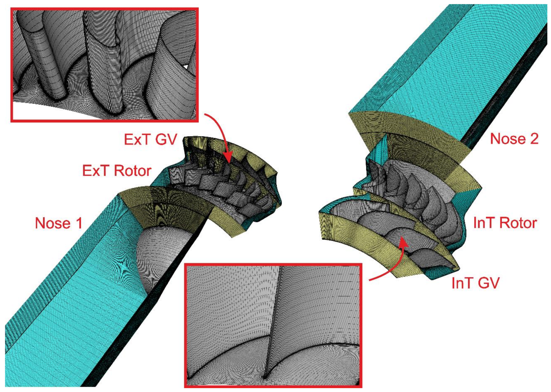
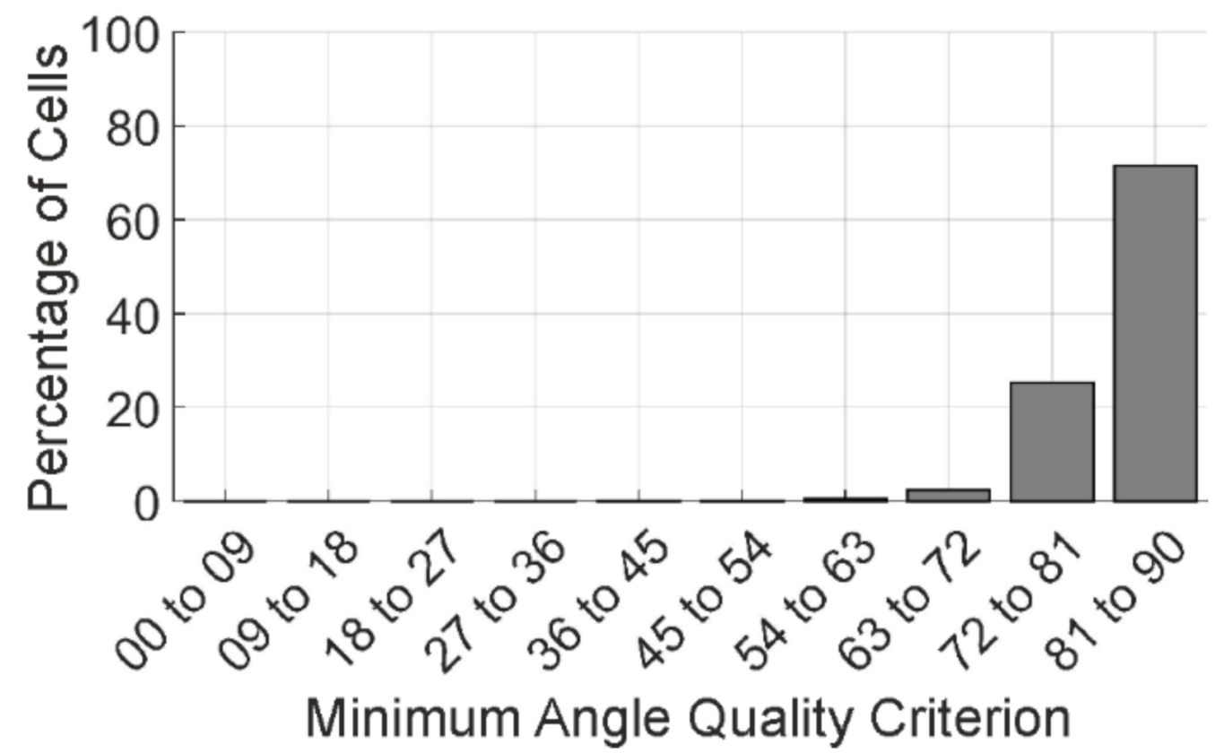
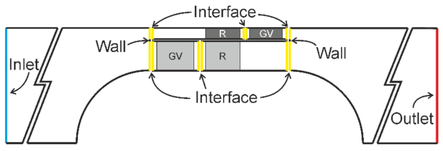
3. Numerical CFD Model

The design of the DDT geometry has been inspired in a unidirectional axial turbine taken from the bibliography [25] but introducing a slight modification in the solidity of the guide vanes (GV) as proposed in [26]. In particular, the inlet turbine (InT) is a 1:1 reproduction of this solution, composed of a 24-bladed rotor with 30 inlet guide vanes, while the external turbine (ExT) has been developed as a scaled model of the same geometry but with a larger diameter and a 36-bladed rotor with 30 GVs to maintain the same solidity as in the InT. Furthermore, the blade profiles of both turbines were analyzed in previous works. Both GV profiles (InT and ExT) are equal and taken from [26]. The profile of the InT rotor is also based on the geometry used in [26], while the ExT rotor is a slight modification of that one but with a different trailing edge angle to minimize the kinetic energy loss at the exit (this improvement was presented in [23]). The main geometrical parameters, shown in Figure 2 are summarized in Table 1, including the chord lengths of blades and vanes and the different diameters of the double decker. More information about the design process can be found in [23].
An URANS simulation of this DDT design was carried out to simulate the performance of the turbine for different flow conditions. Taking advantage of the blade/vane count ratios of the turbine, a reduced computational domain comprising only one sixth of the full annulus was finally implemented. Hence, the circumferential domain between the periodic boundaries is composed of six blades and five GVs for the ExT and five blades and four GVs for the InT, thus resulting in 20 passages for the whole modelled geometry.
An analytical estimation of the combined performance of both InT and ExT units, operating separately, was already assessed in a previous work [23], although it was not considering the mixing-out mechanisms of the flow coming from both turbines at the diffusers. To overcome this limitation, two additional bodies composed of a nose and a duct have been respectively included upstream and downstream of the rotor and guide vanes domains for the present work.
Therefore, the simulated geometry has been developed with a multiblock strategy dividing the geometry in six parts (identified in Figure 2 with red numbers 1 to 6). ANSYS Turbogrid® was used to mesh the subdomains 2, 3, 4 and 5, while the geometry of these parts was generated by means of the Blade Editor utility, an add-in option of the ANSYS Design Modeller®. Both vanes and blades walls were meshed with near wall refinements to ensure y+ values below 1. Alternatively, the upstream and downstream parts of the turbine (subdomains 1 and 6) were meshed in ANSYS ICEM® employing a blocking technique which provided a high-quality, structured hexametrical grid. Finally, all the parts were assembled to create the complete model and uploaded into ANSYS Fluent® for further simulation. Details of the mesh are shown in Figure 3.
A grid analysis, in terms of quality and elements number, has been performed to judge the accuracy of the grids adopted. Firstly, the minimum angles criterion, one of the mostly used by CFD practitioners, has been followed to compute the minimum internal angle of all the cells. The results, shown in Figure 4, reveal that 71% of the cells are in the range between 81 and 90 degrees, representing an excellent orthogonality, while only a marginal 1% is in the range 18–27 degrees with poor values. Secondly, three meshes maintaining a similar grid distribution, but with overall sizes of 0.7 M, 3 M and 13 M cells respectively (scaled with an approximate cell ratio of 4.3), were tested to check the mesh sensitivity. The comparison was made in terms of the non-dimensional torque coefficient, as a function of the mesh size for the same working point in all the cases (Figure 5). The evolution of this coefficient shows a classical convergence, being the difference between the mesh sizes of 3 M and 13 M below 2% whereas it is of 12% for the smaller mesh. Therefore, the 3 M mesh has been considered as the most suitable in terms of precision and economy and selected to carry out the bulk of the simulations.
With respect to the boundary conditions, Figure 6 shows the different typologies that were implemented in the simulations to model the rotational motion of the rotor blades. Mainly, six interfaces (in yellow in Figure 6 had to be placed between all the subdomains of the geometry in order to allow the unsteady rotation of the turbine using the sliding mesh technique. Note that, between the interfaces of subdomains 1 and 6, a slim wall of 1 mm had to be placed in order to separate the interfaces of both turbines. These walls are also the front faces of the internal wall that separate the InT and the ExT. Subdomains 2 and 5, that correspond to the ExT and InT rotor stages (which are joint together), rotate then in the same direction and at the same rotational speed (ω = 375 rpm). Figure 6 also represents the inlet (blue) and outlet (red) boundary conditions, fixed as a velocity-inlet and a pressure-outlet (atmospheric) respectively. Note that, for the full determination of the performance curves of the DDT, combined operation of the turbines in both direct and reverse modes is required, so it will be necessary to switch the inlet and outlet boundaries correspondingly.
For the turbulence modelling, the realizable k-ε model with the enhanced wall treatment was used due to it is well-known ability and robustness to work properly within turbomachinery environments providing well-tested results [19,20,27,28]. In addition, the model was executed in an unsteady fashion to fully-simulate the rotor-stator interactions in the DDT stages, with a typical time step size of 10−5 s, equivalent to a temporal discretization of 444 time steps per blade event of the external rotor. Other relevant parameters and discretization schemes are summarized in Table 2. Finally, the CFD model of the DDT was simulated in a computer equipped with an Intel i7-6800K processor and 64 GB of DDR4 RAM memory, taking approximately 24 h of CPU time to obtain converged results for each working point.

4. Validation and Results

The numerical results obtained with the CFD model are presented in terms of the non-dimensional coefficients defined in Section 2. It should be noted that positive values of the flow coefficient correspond to the internal mode (IM) of the turbine, that is, the InT working in direct mode and the ExT in reverse operation. Conversely, negative values of the flow coefficient correspond to the external mode (EM) of the turbine, when the ExT is working in direct mode and the InT in reverse mode.

4.1. Validation

For validation purposes, experimental data of an identical ExT, but working as a unique conventional turbine, was taken from previous works of the authors [23]. The uncertainty of the experimental values (blank markers in Figure 7) has been estimated to be in the range of 3–4% for the flow coefficient, 1.9–6.5% for the pressure coefficient and 1.8–7.0% in the torque coefficient, being the larger deviations at high flow coefficients. This dataset has been compared with the numerical performance of the ExT in the DDT prototype when working in direct mode. Figure 7 reveals the good agreement in both torque and pressure coefficients (in this case, the coefficients have been defined considering exclusively the geometrical parameters of the ExT). The RMSE of the data sets reveals an overall value of 0.457 for the torque coefficient and 1.776 for the aerodynamic coefficient. In relative terms, the normalized error (NRMSE) with respect to the mean values is 0.134 for the CT and 0.298 for the CA. Major discrepancies are found between the CFD and the experimental results only in the pressure coefficient, especially at high flow coefficients. This can be associated with an evident geometrical difference between the experimental and numerical models. In the CFD model, the transition from the annular section of the ExT to the full-annulus area has been modelled through both lateral diffusers, while in the experimental prototype the flow enters and exits the external turbine fully axial without diffusion effects at both sides.

4.2. Performance Curves and Flow Rate Distribution

After validation, the DDT performance curves were numerically obtained and shown in Figure 8. Note that these results are a consequence of the combined operation of both ExT and InT units. Moreover, it is quite expectable that the DDT will not present symmetric behavior in both modes because of the different size of both InT and ExT geometries. This effect is confirmed in all the non-dimensional coefficients, with slight differences between the distributions for the IM (ɸ > 0) and for the EM (ɸ < 0).
The input coefficient of the DDT is conditioned by the turbine which is blocking the flow. The ExT presents a higher blockage capacity than the InT, so in the IM, when the ExT is blocking the flow, the input coefficient is greater than in the EM. This effect has also been seen in previous works [23]. It can be seen that the torque coefficient in IM is lower than in EM because of the lower torque coefficient of the InT during the IM, and also due to the major negative torque coefficient of the ExT while it is blocking the flow (Figure 8). The combination of these two effects explains the difference in the total-to-static efficiency between IM and EM. This unbalanced characteristic between operation at ɸ > 0 and ɸ < 0 suggests the need for a future redesign of the turbines in order to balance the working capacity of the DDT and improve its performance at the same time.
Due to the unique geometry of the DDT, the flow rate distribution across the ExT and InT plays an important role in analyzing the flow patterns of the turbine. Figure 9 shows the percentage of flow across each turbine for all the flow rates simulated. It is concluded from the graph that the InT in its reverse mode (left graph, light purple bar) has a 3% higher flow rate than the ExT in IM (right graph, dark green bar) on average through the flow coefficients above 0.4. However, for the lower flow coefficients (ɸ < 0.4) the ExT in IM (right graph, dark green bar) blocks the flow more efficiently that the InT in EM (left graph, light purple bar). Another important feature is that the EM (left graph) flow distribution tendency is more stable than the IM (right graph), which starts at a greater value and decreases as the flow coefficient grows. These are facts that need to be taken into account for further analysis.
In Figure 8, the IM is clearly influenced by this effect. At lower flow coefficients, it can be seen that the InT has a greater torque than the ExT in EM for the same coefficients (ɸ < 0.4). This is consistent with the better flow rate ratio during the IM in this flow coefficient range, which produces more torque in the InT. Nevertheless, due to the negative torque of the ExT in IM, the whole DDT presents a lower efficiency for these flow coefficients. In addition, at greater flow coefficients, the flow ratio does not benefit the IM at the same time that the torque coefficient produced by the InT is lower than the one produced by the ExT in EM for the same range (ɸ > 1). Both phenomena acting together explains the difference in efficiency between IM and EM (Figure 8). In the other mode, and for the lower flow coefficients, even if the flow ratio is worse than in the same ɸ for the IM, the torque reduction due to the turbine in reverse mode (in this case the InT) is lower than in the IM. Consequently, the EM efficiency at the peak value is 10% higher than in the IM mode. As the flow coefficient rises in EM, the flow ratio decrease is lower, at the same time that the ExT produces more torque coefficient. Thus, the efficiency for the maximum flow coefficient in EM is similar to the peak efficiency of the IM.

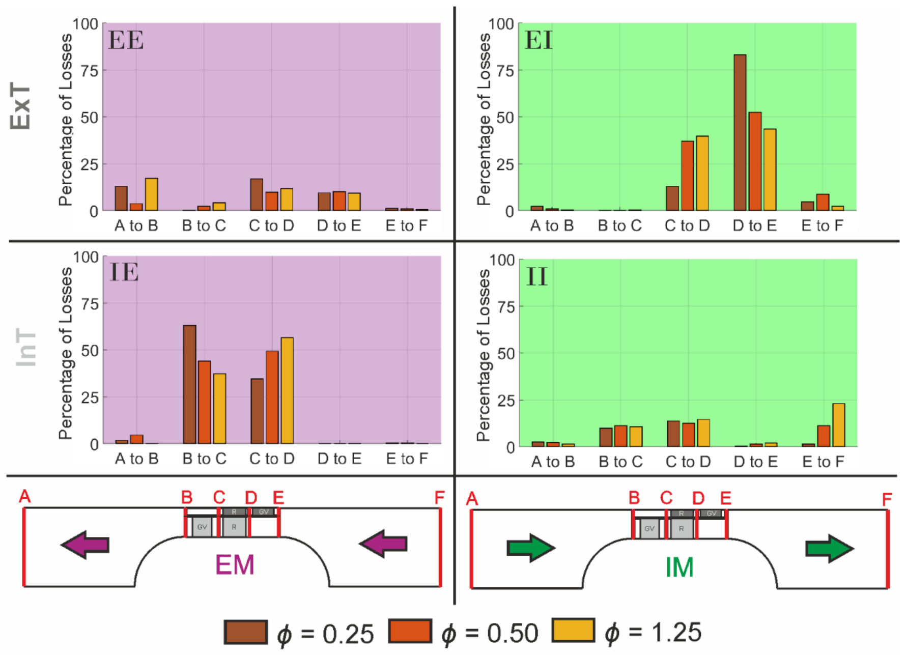
4.3. Pressure Losses Diagram

The distribution of total-to-total pressure losses across the different sections of the DDT provides valuable information about the performance of both internal and external turbines as a function of the flow direction. Hence, Figure 10 shows the pressure losses for both turbines (upper row for ExT and lower row for InT) from inlet to outlet sections (identified as letters A to F in the sketches at the bottom). The left column corresponds to the external mode (EM) while the right column shows the values of the internal mode (IM). To improve the analysis, the extracted energy from both rotors was not taken into account, neither to assess the rotor loss nor to calculate the percentage values. In addition, the data has been represented for three different flow coefficients: ɸ = 0.25 (in brown, below the BEP), ɸ = 0.50 (in orange, for the BEP) and ɸ = 1.25 (in yellow, over the BEP). For a better readability, the four quadrants are denoted as EE (ExT in EM), IE (InT in EM), EI (ExT in IM) and II (InT in IM). The next subsections refer to this designation for simplicity in the explanations.
Note that higher losses in percentage are obviously observed in both EI and IE quadrants when both ExT and InT are working as backflow preventers (higher losses in sections C to E and D to B respectively, that are associated to a severe blockage of the flow). In the case of the EE and II quadrants in the figure both turbines are working in their respective direct modes.
Comparing quadrants IE and EI with the previous presented Figure 9, it can be seen that both turbines present the same tendency. For the lower coefficients, a major part of the blockage is achieved in the GV (quadrant EI, D to E and quadrant IE, B to C). As the flow coefficient goes larger, the losses of the GV decrease at the same time that the rotor losses increase. This tendency is similar to the one followed by the flow distribution. It is confirmed that the flow distribution gets worse if the blockage is mainly made by the rotor. In addition, the maximum value of the flow ratio is reached at the low flow coefficients of the IM, which coincide with the maximum value of losses on the GV (quadrant EI, D to E, brown bar).
The direct modes of the ExT and the InT are shown in quadrants EE and II. The BEP of the ExT is clearly represented in the figure, as the losses in and downstream of the rotor present a minimum in the middle flow coefficient. Nevertheless, for the InT, this point is not so evident, since the kinetic energy at the exit of the rotor (quadrant II, E to F) presents the minimum in the lowest flow coefficient. A study of the angles, at both inlet and outlet zones of the rotor, will be carried out in the future to analyze this point deeper.

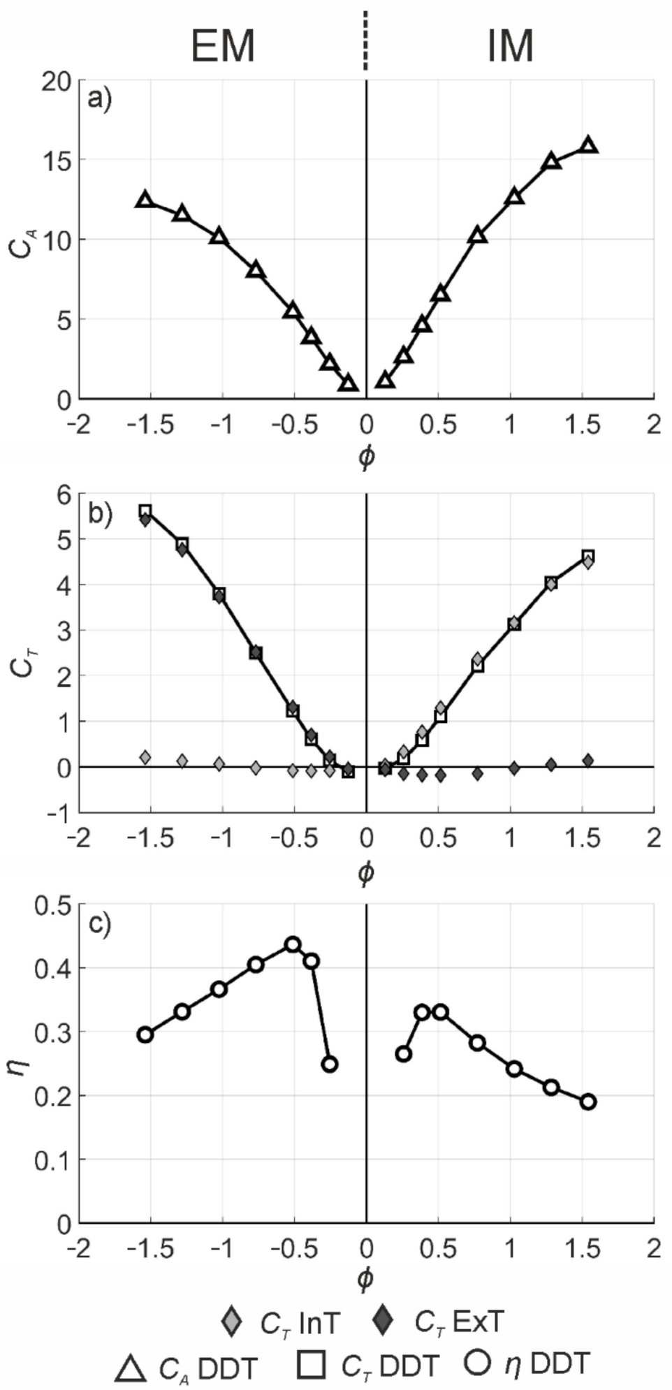
4.4. Rotor Efficiency

The better performance of the ExT rotor in direct mode (during EM) can also be observed in Figure 11, where the efficiency of both rotors (for direct mode only) is represented. Note that for simplicity of the figure, EM flow coefficients (negative values) are also represented in the positive axis. It is clearly shown that the ExT rotor has a greater efficiency for most of the flow coefficients, though the peak efficiency is similar for both rotors. As the ExT has a lower blade span, three-dimensional effects in the turbine are minimized, which leads to a better performance. This difference in the rotor efficiency is explained by this blade span difference.
It is relevant that the InT in IM has a greater rotor efficiency for low flow coefficients (Figure 11) and a better flow distribution ratio for ɸ < 0.4 (Figure 9). However, the negative torque of the ExT in IM deteriorates the overall efficiency of the DDT in these flow coefficients. Additionally, the ExT in EM does not exploit low flow coefficients, due to the negative value of the torque in these ranges. For ɸ < 0.3, the ExT in EM rotor efficiency is negative because the turbine is not extracting energy from the flow (this can also be seen in Figure 11).

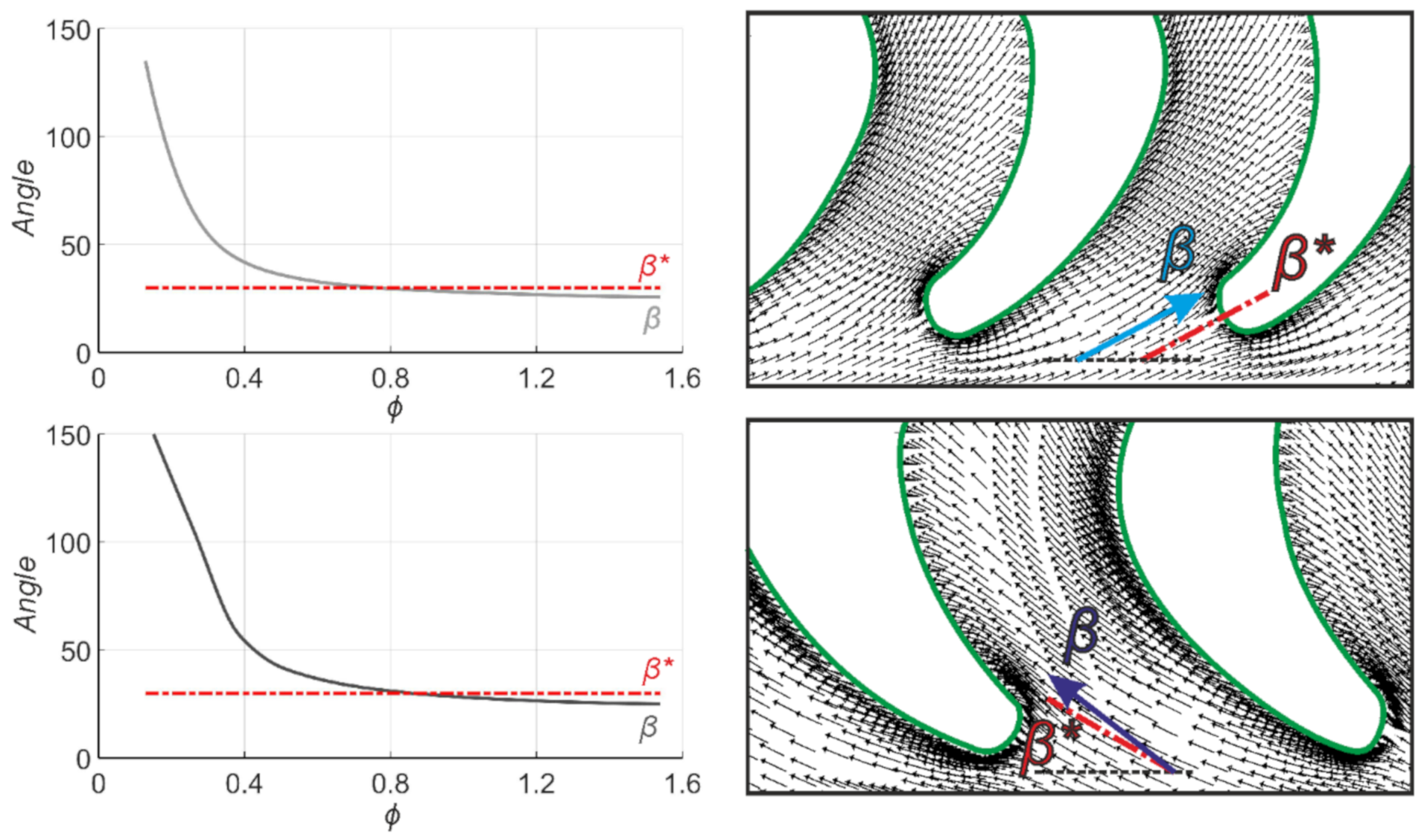
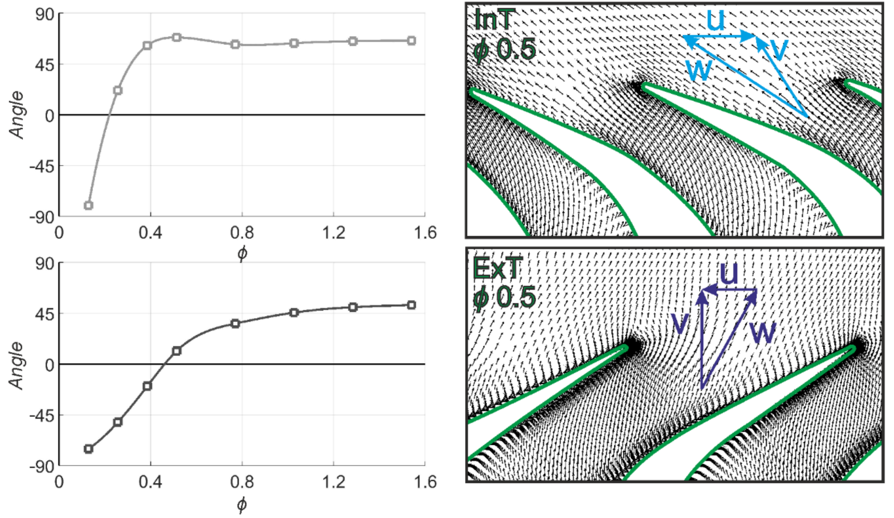
4.5. Rotor Entry and Exit Angles

Additional insight into the aerodynamics of the ExT and InT can be made analyzing the incoming flow angle when both units are working in direct mode (quadrants EE and II). Figure 12 compares the flow angle (β) obtained from the simulations with respect to the geometrical angle of the blades (β*) for the whole range of flow coefficients in direct mode. In the upper plot, the results are shown for the internal turbine (in light grey), while the comparison for the external turbine (in dark grey) is performed in the lower plot.
It can be noticed that the incidence of the flow at the leading edge of the InT is +5° at the design point (ɸ = 0.5). On the contrary, the incidence at the ExT rotor entry is +11° for the BEP (ɸ = 0.5). Both values are not in the optimum range according to the literature. Despite not being in the optimum range, +5° is closer than +11° as the optimum range of incidence goes from −20° to 3.6°, established by [29].
Attending to the lower flow coefficients (below the BEP), the entry angle of the ExT starts in a greater value than the InT one and it keeps greater in all the range. This greater angle leads to a position of the stagnation point in the suction side of the rotor blade, which produces the negative torque of the ExT in EM at lower flow coefficients (also seen in [30]).
A modification in the ExT GV design, decreasing slightly the setting angle of the GV, is expected to minimize the negative torque at low flow coefficients by moving the stagnation point towards the leading edge of the rotor blade. This will allow better efficiency of the DDT at EM. Furthermore, this improvement may also have a beneficial impact for the turbine blockage in reverse mode (IM), inducing more energy losses and a further rise in the overall efficiency of the DDT.
Figure 13 compares the angle of the flow at the exit of the GV (α) with respect to the geometric angle (α*) for both turbines, when they are working in direct mode (quadrants II and EE). It can be seen that the ExT GV redirects the flow as intended, while the InT GV has a tiny mismatch (3°) that does not make a big difference from the point of view of performance. As the GV has a good design, the large incidence observed in Figure 12 is caused merely because of the setting angle of the GV, which should be optimized. Also, according to the data shown in Figure 13, the solidity of the ExT GV could be decreased without losing the guidance, to reduce the losses in EM. Nevertheless, this will influence the blockage of the turbine in IM, changing the flow ratio. Therefore, in the case of the DDT, the solidity of the elements must be studied thoroughly.
The analysis of the exit flow angles of the rotor in direct mode (quadrants II and EE) was also performed for both turbines in Figure 14. The top plot corresponds to the results for the InT (in light grey), while the bottom plot provides the values computed for the ExT (dark grey).
With respect to the InT in IM (quadrant II), Figure 10 demonstrates that the design flow coefficient (ɸ = 0.5) provides a maximum rotor efficiency because of the minimum value of the losses (see bar graphs from C to D, in II). However, there is also an important loss of energy at the diffuser (as revealed in the bar graphs from E to F in II), associated with a high intensity swirl at the exit of the turbine. In Figure 14 (top plot), the InT exit flow angle confirms this feature, showing an evident flow departure from the axial direction (fully axial flow is only attained at ɸ = 0.25). As a consequence, a redesign of the trailing edge angle seems to be necessary in order to increase the peak efficiency at the BEP. Also, the geometry of the diffuser plays an important role in the post swirl of the turbine, so future designs should take care of it to minimize the losses.
Additionally, due to the fully axial direction flow achieved at low flow coefficients, the flow deflection for these coefficients is greater than in the ExT, as well as the torque. This is in concordance with the peak rotor efficiency (Figure 11), where the peak efficiency is reached earlier by the InT than the ExT.
Similar effects are also discussed for the ExT during EM (quadrant EE in Figure 10). Again, the design flow coefficient corresponds to the lower losses at the rotor (C to D in EE), resulting in the maximum rotor efficiency. In this case, the post swirl (A to B in EE) of the ExT is practically minimized at the design point, thus revealing that the outlet velocity has a minimum tangential component. This can be observed in Figure 14 (bottom plot), with a roughly zero exit angle at ɸ = 0.5.

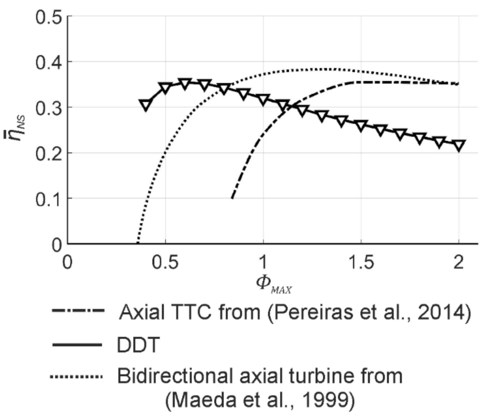
4.6. Non-Steady Efficiency

To conclude the analysis, the non-steady efficiency of the DDT was calculated from the numerical resolution of Equations 5 and 6, assuming a typical sinusoidal flow input from the OWC chamber. The maximum efficiency is practically attained at a flow coefficient amplitude of 0.5 for both ExT and InT units, with maximum values around 35%. These values are found to be similar to those calculated in previous works [23]. In Figure 15 the DDT is compared with an axial bidirectional turbine taken from the bibliography [31] and with the axial TTC from [26]. It can be noticed that the DDT has a peak efficiency similar than the other turbines, but with the peaks placed at different ΦMAX. However, the DDT does have some problems, like the mismatch between the IM and the EM, which at the same time influences the non-steady efficiency. However, achieving symmetric behavior of the turbine (IM and EM) is extremely complex because both units (InT and ExT) cannot have the same geometry due to their different radii and blade spans. Taking this into account, the DDT efficiency should be enhanced in future works trying to improve the IM. It is important to highlight that the numerical model of the DDT, presented in this work, comprises both diffusers and reduces the overall efficiency. This has not been considered in other works.
Figure 16 shows the evolution of the dimensionless coefficients (Φ, CA and CT) during one wave period in order to show the evident mismatch between both IM and EM modes. The second half of the wave (EM mode) has a slightly higher torque coefficient and a lower input coefficient, which leads to a superior performance of the EM mode, according to the results previously exposed.

5. Conclusions

In the present work, the performance of a DDT—a brand new typology of turbine for OWC devices—has been obtained via numerical simulation. In particular, the complete DDT, comprising both internal and external turbines arranged concentrically to guarantee a bidirectional operation using unidirectional flow turbines, has been modelled successfully with an URANS simulation at different flow coefficients.
In addition, a complete analysis of the DDT performance has been carried out in terms of distribution of losses and flow characteristics throughout the turbines. The analysis allowed the identification of several detrimental effects having an impact on the overall efficiency of the prototype. The IM was found to have worse efficiency than the EM, suggesting the need for a redesign of the DDT geometry. In particular, the trailing edge angle of the InT must be increased to reach the totally axial flow at the design point, so the maximum efficiency could be improved. Another significant limitation of the current DDT model is related to the excessive negative torque of the ExT at lower flow coefficients, mainly generated by the flow angle at the entry. A reduction in the trailing angle of the GV would improve the rotor efficiency and would increase the blockage capacity of the ExT and, hence, the global performance of the DDT. On the other hand, the balance between both modes has to be analyzed to ensure symmetric behavior of the DDT, thus enhancing the non-steady efficiency.
On the other hand, a comprehensive solidity study of the different blade/vane rows can enhance the efficiency of the EM or IM. Nevertheless, this study must take into account that any change in the solidity will affect both modes, direct and reverse, of both turbines, InT and ExT.
Despite the existence of several possible improvements, the DDT has proven itself to be a competitive option among other axial turbines designed for OWC systems. In future works, all these suggested ideas will be introduced in a redesign of the DDT and characterized numerically for comparison with the original prototype and with other turbine solutions usually employed as the PTO equipment in OWC devices.

Author Contributions

Conceptualization, M.G.-D. and B.P.; methodology, M.G.-D., C.M.-G. and L.R.; software, M.G.-D. and C.M.-G.; validation, L.R.; formal analysis, C.M.-G.; investigation, C.M.-G.; resources, L.R.; data curation, L.R.; writing—original draft preparation, J.F.-O.; writing—review and editing, J.F.-O.; supervision, B.P. All authors have read and agreed to the published version of the manuscript.

Funding

Manuel García-Díaz is supported by the Spanish ‘‘Ministerio de Educación, Cultura y Deporte’’ within the ‘‘FPU’’ Program (grant number FPU15/04375). Celia Miguel-González is supported by the Spanish “Ministerio de Educación Cultura y Deporte” within the “Doctorados Industriales” Program (grant number DI-17-09596).

Conflicts of Interest

The authors declare no conflict of interest.

Nomenclature

AR = π·(rEX2rIN2) Cross-Flow Area (m2)
cBlade Chord(m)
CADimensionless Input Coefficient(-)
CTDimensionless Torque Coefficient(-)
DDiameter(m)
DREFReference Diameter(m)
NNumber of Blades(-)
ΔPTotal to Static Pressure Difference(Pa)
QFlow Rate(m3s−1)
QExTFlow Rate across the ExT(m3s−1)
QInTFlow Rate across the InT(m3s−1)
QTOTTotal Flow Rate across the DDT(m3s−1)
rmMean Radius(m)
rREFReference Radius(m)
rEXExternal Radius of the ExT(m)
rINInternal Radius of the InT(m)
TWave Period(s)
tTime(s)
T0Torque(Nm)
TExTTorque of the ExT(Nm)
TInTTorque of the InT(Nm)
TTOTTorque of the DDT(Nm)
uRTangential Velocity at rREF(ms−1)
vaVelocity at AR(ms−1)
ωRotational Speed(rads−1)
ρAir Density(kgm−3)
ɸSteady Dimensionless Flow Coefficient(-)
ηTotal-to-Static Steady Efficiency(-)
η ¯ NSNon-Steady Efficiency(-)
η ¯ InputInput efficiency(-)
η ¯ tgNet efficiency of the DDT(-)
ΦNon-steady Dimensionless Flow Coefficient(-)
ΦMAXMaximum value of Φ(-)
BEPBest Efficiency Point(-)
DDTDouble Decker Turbine(-)
ExTExternal Turbine(-)
GVGuide Vanes(-)
InTInternal Turbine(-)
NRMSENormalized Root-Mean Squared Error(-)
OWCOscillating Water Column(-)
PTOPower-Take-Off(-)
RMSERoot-Mean Squared Error(-)
TTCTwin Turbines Configuration(-)
WECWave Energy Converter(-)

References

  1. Astariz, S.; Iglesias, G. The economics of wave energy: A review. Renew. Sustain. Energy Rev. 2015, 45, 397–408. [Google Scholar] [CrossRef]
  2. Melikoglu, M. Current status and future of ocean energy sources: A global review. Ocean Eng. 2018, 148, 563–573. [Google Scholar] [CrossRef]
  3. Falcão, A.F.O.; Gato, L.M.C. Chapter 8.5: Air Turbines. In Comprehensive renewable energy; Sayigh, A., Ed.; Elsevier: Amsterdam, The Netherlands, 2012; Volume 8, pp. 1–39. ISBN 9780080878737. [Google Scholar]
  4. Setoguchi, T.; Takao, M. Current status of self-rectifying air turbines for wave energy conversion. Energy Convers. Manag. 2006, 47, 2382–2396. [Google Scholar] [CrossRef]
  5. Takao, M.; Setoguchi, T. Air turbines for wave energy conversion. Int. J. Rotating Mach. 2012, 2012, 10. [Google Scholar] [CrossRef] [Green Version]
  6. Ansarifard, N.; Kianejad, S.S.; Fleming, A.; Chai, S. A radial inflow air turbine design for a vented oscillating water column. Energy 2019, 166, 380–391. [Google Scholar] [CrossRef]
  7. Okuhara, S.; Takao, M.; Sato, H.; Takami, A.; Setoguchi, T. A Twin Impulse Turbine for Wave Energy Conversion—Effect of Fluidic Diode Geometry on the Performance. Open J. Fluid Dyn. 2014, 4, 433–439. [Google Scholar] [CrossRef] [Green Version]
  8. Bruschi, D.L.; Fernandes, J.C.S.; Falcão, A.F.O.; Bergmann, C.P. Analysis of the degradation in the Wells turbine blades of the Pico oscillating-water-column wave energy plant. Renew. Sustain. Energy Rev. 2019, 115, 109368. [Google Scholar] [CrossRef]
  9. Wells, A.A. Fluid driven rotary transducer. Br. Pat. spec 1976, 1, 595–700. [Google Scholar]
  10. Raghunathan, S. the Wells Air Turbine for Wave Energy Conversion. Prog. Aerosp. Sci. 1995, 31, 335–386. [Google Scholar] [CrossRef]
  11. Ibarra-Berastegi, G.; Sáenz, J.; Ulazia, A.; Serras, P.; Esnaola, G.; Garcia-Soto, C. Electricity production, capacity factor, and plant efficiency index at the Mutriku wave farm (2014–2016). Ocean Eng. 2018, 147, 20–29. [Google Scholar] [CrossRef] [Green Version]
  12. Kumar, P.M.; Halder, P.; Husain, A.; Samad, A. Performance enhancement of Wells turbine: Combined radiused edge blade tip, static extended trailing edge, and variable thickness modifications. Ocean Eng. 2019, 185, 47–58. [Google Scholar] [CrossRef]
  13. Babintsev, I.A. Apparatus for Converting Sea Wave Energy into Electrical Energy. Patent No. US3922739A, 12 February 1975. [Google Scholar]
  14. López, I.; Andreu, J.; Ceballos, S.; Martínez De Alegría, I.; Kortabarria, I. Review of wave energy technologies and the necessary power-equipment. Renew. Sustain. Energy Rev. 2013, 27, 413–434. [Google Scholar] [CrossRef]
  15. Jayashankar, V.; Anand, S.; Geetha, T.; Santhakumar, S.; Jagadeesh Kumar, V.; Ravindran, M.; Setoguchi, T.; Takao, M.; Toyota, K.; Nagata, S. A twin unidirectional impulse turbine topology for OWC based wave energy plants. Renew. Energy 2009, 34, 692–698. [Google Scholar] [CrossRef]
  16. Falcão, A.F.O.; Henriques, J.C.C. Oscillating-water-column wave energy converters and air turbines: A review. Renew. Energy 2016, 85, 1391–1424. [Google Scholar] [CrossRef]
  17. Falcão, A.F.O.; Gato, L.M.C.; Henriques, J.C.C.; Borges, J.E.; Pereiras, B.; Castro, F. A novel twin-rotor radial-inflow air turbine for oscillating-water-column wave energy converters. Energy 2015, 93, 2116–2125. [Google Scholar] [CrossRef]
  18. Falcao, A.F.O.; Gato, L.M.C. Turbine with radial inlet and outlet rotor for use in bidirectional flows. Patent No. EP2538070B1, 12 February 1975. [Google Scholar]
  19. Ansarifard, N.; Fleming, A.; Henderson, A.; Kianejad, S.S.; Chai, S.; Orphin, J. Comparison of inflow and outflow radial air turbines in vented and bidirectional OWC wave energy converters. Energy 2019, 182, 159–176. [Google Scholar] [CrossRef]
  20. Rodríguez, L.; Pereiras, B.; Fernández-Oro, J.; Castro, F. Optimization and experimental tests of a centrifugal turbine for an owc device equipped with a twin turbines configuration. Energy 2019, 171, 710–720. [Google Scholar] [CrossRef] [Green Version]
  21. Lopes, B.S.; Gato, L.M.C.; Falcão, A.F.O.; Henriques, J.C.C. Test results of a novel twin-rotor radial inflow self-rectifying air turbine for OWC wave energy converters. Energy 2019, 170, 869–879. [Google Scholar] [CrossRef]
  22. García Díaz, M.; Rodriguez, L.; Pereiras, B. Turbina para aprovechamiento de flujo bidireccional. Patent No. ES2729207B2, 2018. [Google Scholar]
  23. Garcia-Diaz, M.; Pereiras, B.; Miguel-Gonzalez, C.; Rodriguez, L.; Fernandez-Oro, J. Design of a new turbine for OWC Wave Energy Converters: The DDT concept. Renew. Energy 2021. accepted for publication. [Google Scholar] [CrossRef]
  24. Rodríguez, L.; Pereiras, B.; Fernández-Oro, J.; Castro, F. Viability of unidirectional radial turbines for twin-turbine configuration of OWC wave energy converters. Ocean Eng. 2018, 154, 288–297. [Google Scholar] [CrossRef]
  25. Takao, M.; Takami, A.; Okuhara, S.; Setoguchi, T. A twin unidirectional impulse turbine for wave energy conversion. J. Therm. Sci. 2011, 20, 394–397. [Google Scholar] [CrossRef]
  26. Pereiras, B.; Valdez, P.; Castro, F. Numerical analysis of a unidirectional axial turbine for twin turbine configuration. Appl. Ocean Res. 2014, 47, 1–8. [Google Scholar] [CrossRef]
  27. Thakker, A.; Dhanasekaran, T.S. Computed effects of tip clearance on performance of impulse turbine for wave energy conversion. Renew. Energy 2004, 29, 529–547. [Google Scholar] [CrossRef]
  28. Cui, Y.; Liu, Z.; Zhang, X.; Xu, C. Review of CFD studies on axial-flow self-rectifying turbines for OWC wave energy conversion. Ocean Eng. 2019, 175, 80–102. [Google Scholar] [CrossRef]
  29. Cho, S.Y.; Choi, S.K. Experimental study of the incidence effect on rotating turbine blades. Proc. Inst. Mech. Eng. Part A J. Power Energy 2004, 218, 669–676. [Google Scholar] [CrossRef]
  30. Thakker, A.; Jarvis, J.; Sahed, A. Quasi-steady analytical model benchmark of an impulse turbine for wave energy extraction. Int. J. Rotat. Mach. 2008, 2008, 12. [Google Scholar] [CrossRef] [Green Version]
  31. Maeda, H.; Santhakumar, S.; Setoguchi, T.; Takao, M.; Kinoue, Y.; Kaneko, K. Performance of an impulse turbine with fixed guide vanes for wave power conversion. Renew. Energy 1999, 17, 533–547. [Google Scholar] [CrossRef]
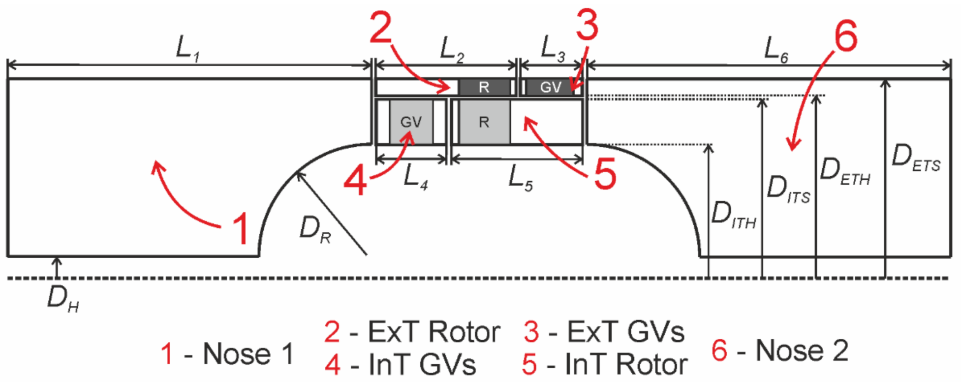
Figure 1. Base scheme and performance of the Double Decker Turbine (DDT). Note that large arrows correspond to the direct mode of each stage and small ones to the reverse mode.
Energies 14 00949 g001
Figure 2. Main geometric parameters and assembly of the meshes to conform the DDT.
Energies 14 00949 g002
Figure 3. Details of the mesh.
Energies 14 00949 g003
Figure 4. Quality of the mesh in terms of the minimum angles criterion.
Energies 14 00949 g004
Figure 5. Mesh sensitivity analysis for ɸ = 0.5.
Energies 14 00949 g005
Figure 6. Boundary conditions of the simulations.
Energies 14 00949 g006
Figure 7. Comparison between numerical and experimental data for: (a) the input; (b) torque dimensionless coefficients of the ExT. Blank markers correspond to experimental data and solid markers to numerical data.
Energies 14 00949 g007
Figure 8. Performance curves of the DDT: (a) Input coefficient; (b) Torque coefficient; (c) Efficiency. Negative flow coefficients correspond to EM and positive ones to IM.
Energies 14 00949 g008
Figure 9. Percentage of the flow across each turbine for both modes.
Energies 14 00949 g009
Figure 10. Losses diagram for the DDT in both modes. Note that is the columns represent the mode (IM on the left and EM on the right) and the rows show information about both turbines (InT on the bottom and ExT on the top).
Energies 14 00949 g010
Figure 11. Total-to-total rotor efficiency for InT in IM (light grey) and ExT in EM (dark grey). For simplicity, both modes are represented in the positive axis.
Energies 14 00949 g011
Figure 12. Averaged angles at the leading edge of the rotor blades for the InT (light grey, upper plot) at IM and the ExT (dark grey, lower plot) at EM. 0° corresponds to the tangential direction. Vectors plot are from the midspan section of each turbine at ɸ = 0.5.
Energies 14 00949 g012
Figure 13. Averaged angles at the exit of the guide vanes for the InT (light grey) at IM and the ExT (dark grey) at EM. 0° corresponds to the tangential direction.
Energies 14 00949 g013
Figure 14. Average rotor exit flow angle for InT (light grey) at IM and ExT (dark grey) at EM. 0° corresponds to the axial direction. Vectors plot are from the midspan section of each turbine at ɸ = 0.5.
Energies 14 00949 g014
Figure 15. Comparison between the non-steady efficiency of the DDT, an axial impulse bidirectional turbine from [31] and an axial TTC from [26].
Energies 14 00949 g015
Figure 16. Evolution of the dimensionless coefficients during one wave period.
Energies 14 00949 g016
Table 1. Values of the main geometric parameters.
L1734 mm
L2120 mm
L355 mm
L455 mm
L5120 mm
L6734 mm
DH10 mm
DR190 mm
DITH210 mm
DITS /DREF298 mm
DETH300 mm
DETS367 mm
Number of ExT rotor blades36
Number of ExT guide vanes30
Number of InT rotor blades24
Number of InT guide vanes30
Table 2. Summary of the main simulation parameters.
Turbulence ModelRealizable k-ε with Enhanced Wall Treatment
Pressure-velocity couplingSIMPLE Scheme
Transient formulationSecond order implicit
Spatial Discretization
GradientGreen-Gauss cell based
PressureBody force weighted
MomentumThird-order MUSCL
Turbulent kinetic energyThird-order MUSCL
Turbulent dissipation rateThird-order MUSCL
Publisher’s Note: MDPI stays neutral with regard to jurisdictional claims in published maps and institutional affiliations.

