
Monitoring the Foliar Nutrients Status of Mango Using Spectroscopy-Based Spectral Indices and PLSR-Combined Machine Learning Models


 ,
,  ,
,  , and
, and
Abstract
:
1. Introduction
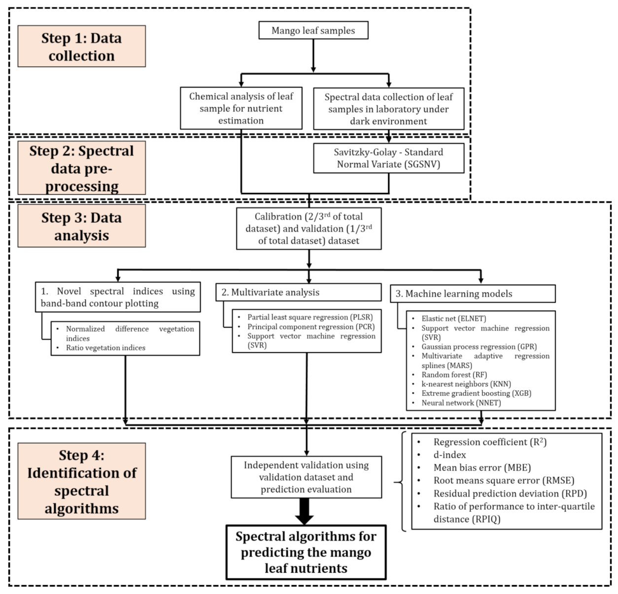
2. Materials and Methods
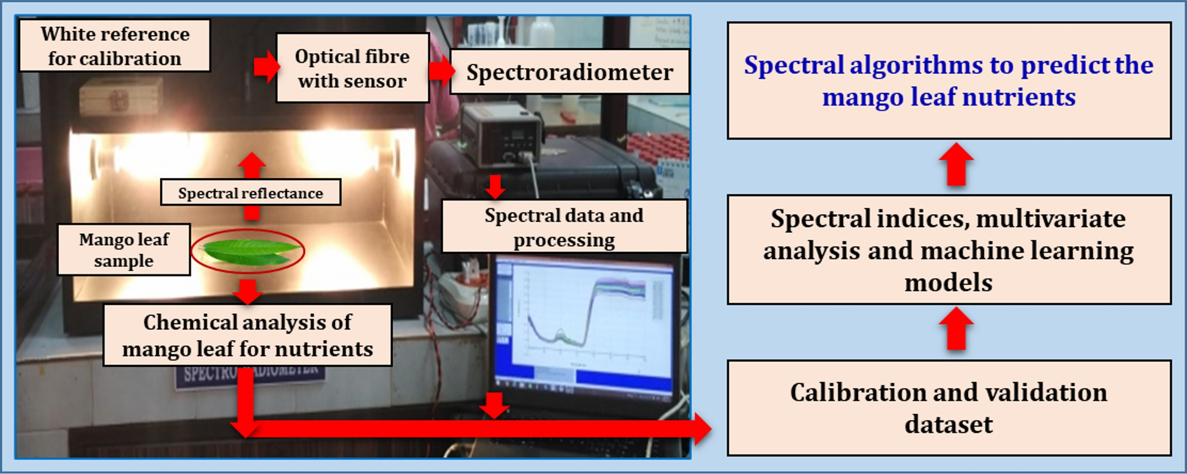
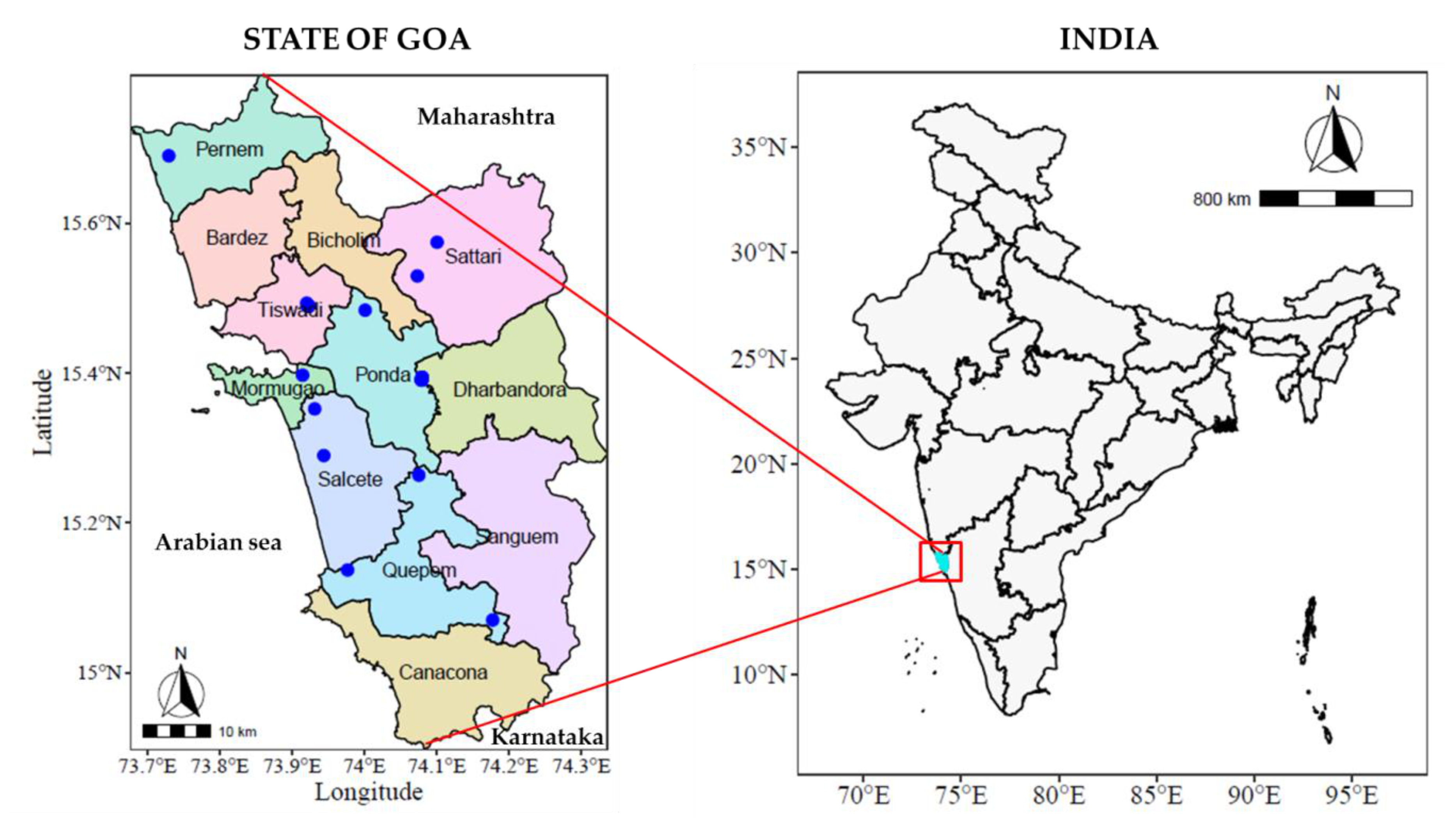
2.1. Experimental Setup
2.2. Spectral Measurements
2.3. Chemical Analysis
2.4. Development of Parametric Regression Models
2.5. Development of Nonparametric Regression Models
3. Results
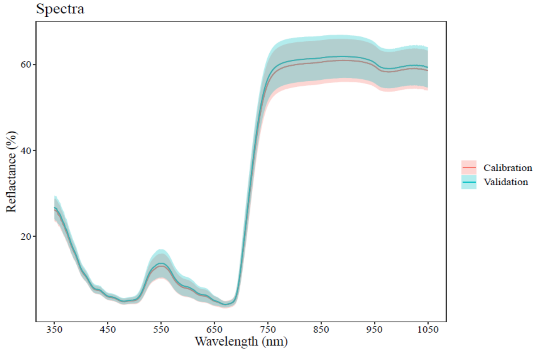
3.1. Descriptive Statistics
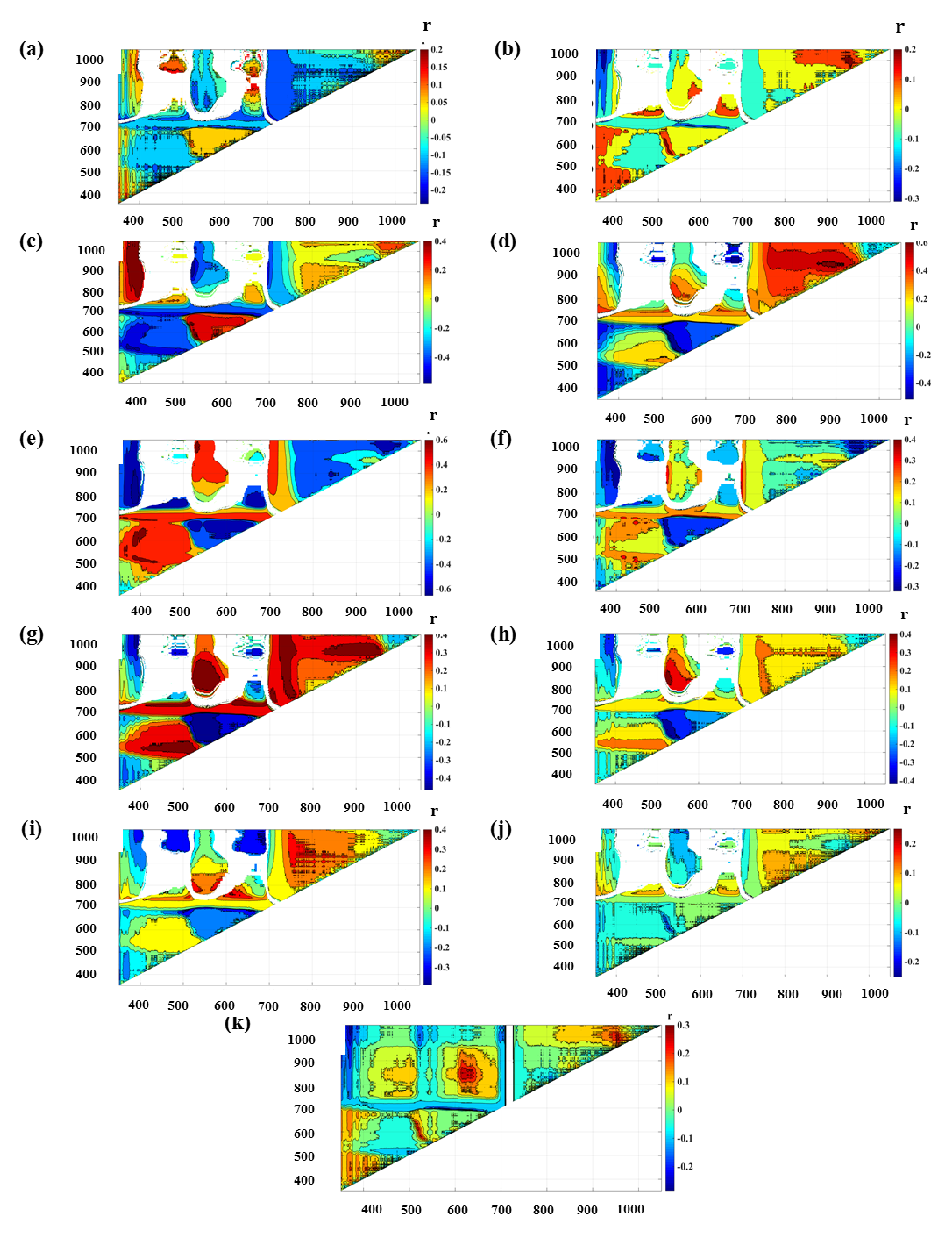
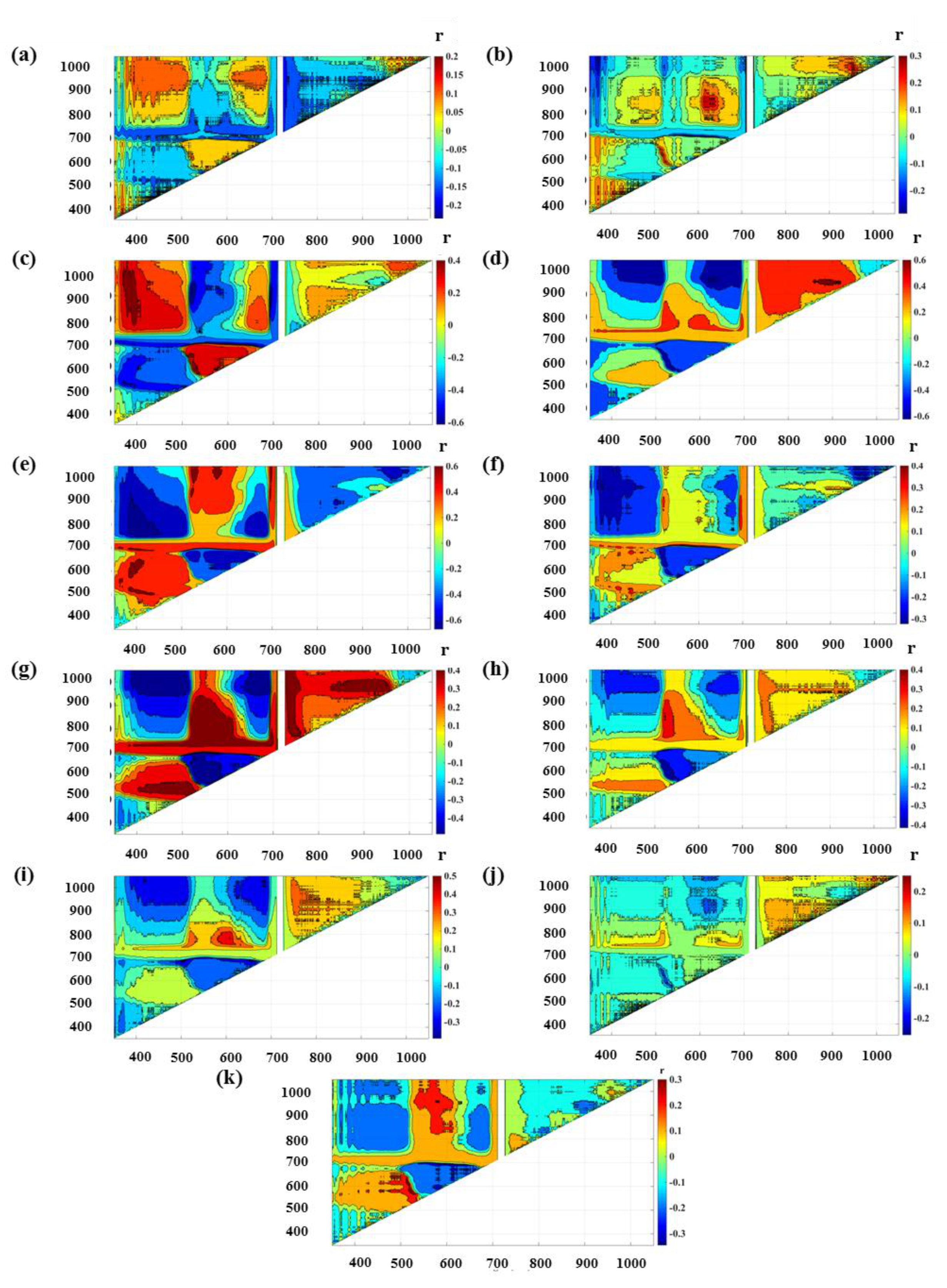
3.2. Indices Development and Prediction Performance
3.3. Performance of Nonparametric Regression Analysis
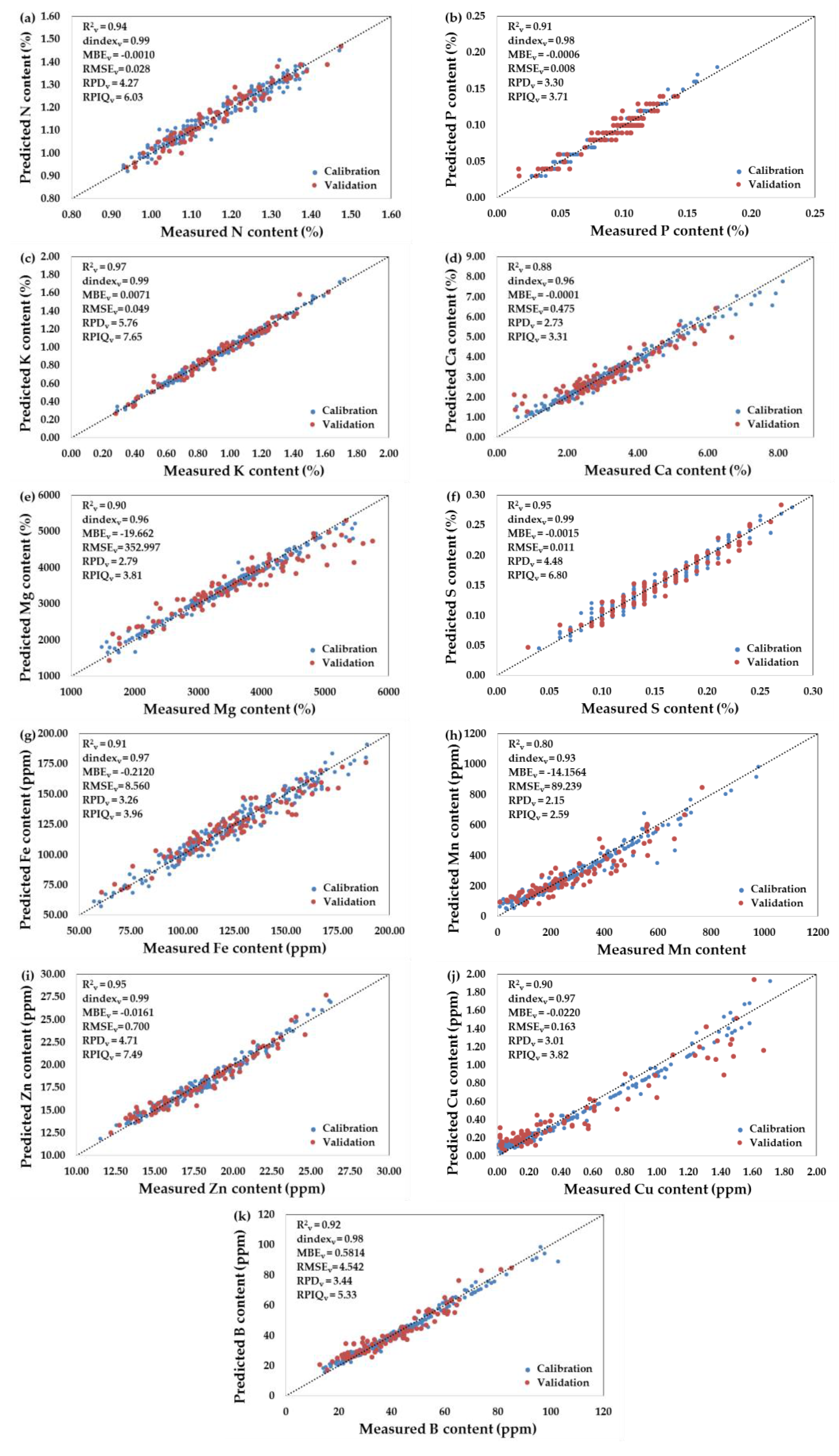
3.4. Performance of the PLSR-Combined Machine Learning Models
4. Discussion
4.1. Variations in Leaf Nutrient Concentrations and Spectral Data
4.2. Vegetation Indices
4.3. Chemometrics and Machine Learning Regression Modeling
5. Conclusions
Author Contributions
Funding
Institutional Review Board Statement
Informed Consent Statement
Data Availability Statement
Acknowledgments
Conflicts of Interest
Appendix A

| Calibration | Validation | ||||||||||||
|---|---|---|---|---|---|---|---|---|---|---|---|---|---|
| R2c | dindex c | MBEc | RMSEc | RPDc | RPIQc | R2v | dindexv | MBEv | RMSEv | RPDv | RPIQv | Summed rank | |
| N | |||||||||||||
| ELNET | 0.95 | 0.99 | −0.0002 | 0.028 | 4.50 | 7.96 | 0.94 | 0.99 | −0.0019 | 0.029 | 4.19 | 5.92 | 38 |
| SVR | 0.98 | 0.99 | −0.0007 | 0.019 | 6.48 | 11.46 | 0.85 | 0.95 | −0.0042 | 0.048 | 2.48 | 3.51 | 37 |
| GPR | 0.96 | 0.97 | −0.0017 | 0.035 | 3.53 | 6.25 | 0.84 | 0.92 | −0.0042 | 0.057 | 2.12 | 3.00 | 67 |
| MARS | 0.80 | 0.94 | −0.0005 | 0.056 | 2.22 | 3.92 | 0.58 | 0.86 | 0.0068 | 0.097 | 1.24 | 1.75 | 93 |
| RF | 0.98 | 0.97 | −0.0011 | 0.035 | 3.51 | 6.21 | 0.72 | 0.75 | 0.0006 | 0.082 | 1.47 | 2.07 | 77 |
| KNN | 0.78 | 0.89 | 0.0007 | 0.066 | 1.89 | 3.35 | 0.55 | 0.81 | −0.0103 | 0.082 | 1.47 | 2.08 | 96 |
| XGB | 0.97 | 0.99 | 0.0012 | 0.023 | 5.36 | 9.48 | 0.77 | 0.93 | 0.0001 | 0.057 | 2.11 | 2.98 | 48 |
| NNET | 0.95 | 0.99 | 0.0085 | 0.028 | 4.38 | 7.75 | 0.95 | 0.99 | 0.0066 | 0.029 | 4.22 | 5.96 | 48 |
| Cubist | 0.95 | 0.99 | 0.0003 | 0.028 | 4.42 | 7.83 | 0.94 | 0.99 | −0.0010 | 0.028 | 4.27 | 6.03 | 36 |
| P | |||||||||||||
| ELNET | 0.94 | 0.99 | 0.0001 | 0.007 | 4.25 | 5.59 | 0.92 | 0.98 | −0.0003 | 0.008 | 3.47 | 3.90 | 28 |
| SVR | 0.97 | 0.99 | −0.0002 | 0.006 | 5.39 | 7.10 | 0.89 | 0.97 | −0.0001 | 0.009 | 3.04 | 3.42 | 35 |
| GPR | 0.95 | 0.97 | 0.0000 | 0.009 | 3.53 | 4.64 | 0.89 | 0.96 | −0.0001 | 0.009 | 2.81 | 3.16 | 54 |
| MARS | 0.76 | 0.93 | 0.0003 | 0.015 | 2.06 | 2.71 | 0.58 | 0.87 | −0.0008 | 0.018 | 1.51 | 1.70 | 89 |
| RF | 0.98 | 0.97 | 0.0003 | 0.009 | 3.34 | 4.40 | 0.79 | 0.79 | 0.0009 | 0.017 | 1.57 | 1.77 | 73 |
| KNN | 0.79 | 0.90 | −0.0010 | 0.016 | 1.95 | 2.57 | 0.65 | 0.85 | 0.0012 | 0.016 | 1.63 | 1.84 | 91 |
| XGB | 0.94 | 0.99 | 0.0001 | 0.007 | 4.18 | 5.50 | 0.77 | 0.93 | 0.0003 | 0.013 | 2.10 | 2.37 | 56 |
| NNET | 0.94 | 0.98 | 0.0007 | 0.007 | 4.14 | 5.45 | 0.91 | 0.98 | 0.0004 | 0.008 | 3.34 | 3.77 | 44 |
| Cubist | 0.98 | 0.99 | −0.0002 | 0.004 | 6.92 | 9.10 | 0.91 | 0.98 | −0.0006 | 0.008 | 3.30 | 3.71 | 24 |
| K | |||||||||||||
| ELNET | 0.98 | 0.99 | −0.0001 | 0.043 | 6.38 | 7.96 | 0.97 | 0.99 | 0.0071 | 0.046 | 6.04 | 8.03 | 25 |
| SVR | 0.99 | 1.00 | −0.0023 | 0.035 | 7.69 | 9.60 | 0.92 | 0.97 | 0.0120 | 0.087 | 3.21 | 4.27 | 44 |
| GPR | 0.98 | 0.98 | −0.0029 | 0.068 | 3.98 | 4.97 | 0.93 | 0.95 | 0.0107 | 0.105 | 2.68 | 3.56 | 65 |
| MARS | 0.83 | 0.95 | −0.0004 | 0.112 | 2.43 | 3.04 | 0.76 | 0.92 | 0.0057 | 0.138 | 2.03 | 2.70 | 79 |
| RF | 0.98 | 0.98 | −0.0022 | 0.074 | 3.70 | 4.61 | 0.78 | 0.80 | 0.0183 | 0.179 | 1.57 | 2.08 | 85 |
| KNN | 0.83 | 0.92 | −0.0087 | 0.126 | 2.16 | 2.69 | 0.62 | 0.82 | 0.0170 | 0.180 | 1.56 | 2.07 | 105 |
| XGB | 0.98 | 0.99 | 0.0012 | 0.043 | 6.34 | 7.91 | 0.82 | 0.95 | 0.0103 | 0.118 | 2.38 | 3.16 | 62 |
| NNET | 0.98 | 0.99 | −0.0105 | 0.045 | 6.01 | 7.50 | 0.97 | 0.99 | −0.0071 | 0.052 | 5.38 | 7.14 | 54 |
| Cubist | 0.99 | 1.00 | −0.0007 | 0.025 | 11.06 | 13.80 | 0.97 | 0.99 | 0.0071 | 0.049 | 5.76 | 7.65 | 21 |
| Ca | |||||||||||||
| ELNET | 0.96 | 0.99 | −0.0107 | 0.322 | 4.70 | 5.58 | 0.94 | 0.98 | −0.0535 | 0.318 | 4.08 | 4.94 | 34 |
| SVR | 0.98 | 0.99 | −0.0214 | 0.238 | 6.36 | 7.54 | 0.88 | 0.96 | 0.0001 | 0.475 | 2.73 | 3.31 | 30 |
| GPR | 0.97 | 0.98 | −0.0683 | 0.422 | 3.59 | 4.25 | 0.88 | 0.93 | −0.0285 | 0.552 | 2.35 | 2.85 | 70 |
| MARS | 0.84 | 0.95 | −0.0337 | 0.609 | 2.49 | 2.95 | 0.66 | 0.90 | 0.0129 | 0.759 | 1.71 | 2.07 | 84 |
| RF | 0.98 | 0.98 | −0.0721 | 0.393 | 3.85 | 4.57 | 0.63 | 0.80 | −0.0814 | 0.852 | 1.52 | 1.84 | 83 |
| KNN | 0.83 | 0.87 | −0.1389 | 0.833 | 1.82 | 2.15 | 0.65 | 0.79 | −0.1060 | 0.867 | 1.50 | 1.81 | 107 |
| XGB | 0.97 | 0.99 | −0.0158 | 0.252 | 6.02 | 7.13 | 0.77 | 0.93 | −0.0712 | 0.624 | 2.08 | 2.52 | 49 |
| NNET | 0.97 | 0.99 | −0.0195 | 0.266 | 5.70 | 6.76 | 0.91 | 0.98 | -0.0125 | 0.382 | 3.39 | 4.11 | 36 |
| Cubist | 0.96 | 0.99 | −0.0273 | 0.324 | 4.68 | 5.55 | 0.94 | 0.98 | −0.0701 | 0.320 | 4.05 | 4.90 | 47 |
| Mg | |||||||||||||
| ELNET | 0.95 | 0.99 | 0.0000 | 190.287 | 4.70 | 6.20 | 0.95 | 0.99 | 28.6533 | 219.943 | 4.47 | 6.11 | 28 |
| SVR | 0.98 | 0.99 | −2.5794 | 133.784 | 6.69 | 8.82 | 0.90 | 0.96 | −19.6623 | 352.997 | 2.79 | 3.81 | 27 |
| GPR | 0.97 | 0.98 | 6.0932 | 226.551 | 3.95 | 5.21 | 0.91 | 0.94 | −2.3241 | 393.767 | 2.50 | 3.41 | 54 |
| MARS | 0.78 | 0.94 | 0.0000 | 414.932 | 2.16 | 2.84 | 0.67 | 0.90 | −39.8115 | 565.089 | 1.74 | 2.38 | 78 |
| RF | 0.98 | 0.98 | 2.9559 | 227.748 | 3.93 | 5.18 | 0.71 | 0.82 | −50.5409 | 618.348 | 1.59 | 2.17 | 77 |
| KNN | 0.80 | 0.90 | 82.2845 | 455.592 | 1.96 | 2.59 | 0.80 | 0.88 | 44.4215 | 528.350 | 1.86 | 2.54 | 84 |
| XGB | 0.97 | 0.99 | -3.8362 | 144.384 | 6.20 | 8.17 | 0.86 | 0.95 | 11.3587 | 381.799 | 2.58 | 3.52 | 39 |
| NNET | 0.04 | 0.45 | −1163.8440 | 1640.410 | 0.55 | 0.72 | 0.07 | 0.47 | -1340.4810 | 1727.948 | 0.57 | 0.78 | 108 |
| Cubist | 0.95 | 0.99 | 19.8129 | 191.229 | 4.68 | 6.17 | 0.95 | 0.99 | 49.4772 | 222.529 | 4.42 | 6.04 | 45 |
| S | |||||||||||||
| ELNET | 0.96 | 0.99 | −0.0001 | 0.009 | 4.95 | 6.55 | 0.95 | 0.99 | −0.0015 | 0.011 | 4.48 | 6.80 | 26 |
| SVR | 0.98 | 0.99 | −0.0002 | 0.007 | 6.18 | 8.18 | 0.87 | 0.96 | −0.0016 | 0.018 | 2.69 | 4.09 | 40 |
| GPR | 0.97 | 0.98 | −0.0006 | 0.013 | 3.62 | 4.79 | 0.89 | 0.93 | −0.0025 | 0.021 | 2.36 | 3.57 | 68 |
| MARS | 0.78 | 0.93 | −0.0006 | 0.021 | 2.13 | 2.82 | 0.62 | 0.88 | −0.0015 | 0.031 | 1.61 | 2.44 | 85 |
| RF | 0.98 | 0.97 | −0.0012 | 0.013 | 3.46 | 4.57 | 0.78 | 0.76 | −0.0069 | 0.033 | 1.48 | 2.25 | 84 |
| KNN | 0.76 | 0.85 | −0.0026 | 0.027 | 1.70 | 2.26 | 0.70 | 0.77 | −0.0083 | 0.034 | 1.46 | 2.22 | 105 |
| XGB | 0.98 | 0.99 | −0.0001 | 0.007 | 6.97 | 9.22 | 0.84 | 0.94 | −0.0015 | 0.020 | 2.42 | 3.68 | 37 |
| NNET | 0.96 | 0.98 | 0.0072 | 0.012 | 3.87 | 5.12 | 0.95 | 0.98 | 0.0057 | 0.012 | 3.99 | 6.05 | 56 |
| Cubist | 0.96 | 0.99 | 0.0003 | 0.009 | 4.86 | 6.43 | 0.95 | 0.99 | −0.0008 | 0.011 | 4.38 | 6.64 | 39 |
| Fe | |||||||||||||
| ELNET | 0.96 | 0.99 | 0.0000 | 5.714 | 4.95 | 7.13 | 0.94 | 0.98 | 0.4834 | 6.649 | 4.19 | 5.10 | 33 |
| SVR | 0.98 | 0.99 | −0.2295 | 4.427 | 6.38 | 9.20 | 0.91 | 0.97 | −0.2120 | 8.560 | 3.26 | 3.96 | 31 |
| GPR | 0.96 | 0.98 | 0.0700 | 7.743 | 3.65 | 5.26 | 0.91 | 0.95 | −0.1209 | 10.470 | 2.66 | 3.24 | 54 |
| MARS | 0.77 | 0.93 | 0.0000 | 13.670 | 2.07 | 2.98 | 0.68 | 0.90 | −0.5475 | 15.952 | 1.75 | 2.13 | 71 |
| RF | 0.98 | 0.98 | −0.1374 | 7.347 | 3.85 | 5.55 | 0.68 | 0.82 | −1.5566 | 17.722 | 1.57 | 1.91 | 70 |
| KNN | 0.76 | 0.89 | −0.1584 | 15.173 | 1.86 | 2.69 | 0.60 | 0.81 | −1.2094 | 18.478 | 1.51 | 1.83 | 93 |
| XGB | 0.97 | 0.99 | 0.1141 | 4.796 | 5.89 | 8.50 | 0.85 | 0.96 | −1.2427 | 10.731 | 2.60 | 3.16 | 47 |
| NNET | 0.22 | 0.68 | −4.9762 | 34.855 | 0.81 | 1.17 | 0.24 | 0.68 | −7.4574 | 33.930 | 0.82 | 1.00 | 108 |
| Cubist | 0.96 | 0.99 | −0.0352 | 5.720 | 4.94 | 7.12 | 0.94 | 0.99 | 0.4824 | 6.580 | 4.23 | 5.15 | 33 |
| Mn | |||||||||||||
| ELNET | 0.75 | 0.88 | -0.5831 | 205.813 | 1.19 | 1.29 | 0.88 | 0.96 | −23.2350 | 70.000 | 2.74 | 3.31 | 50 |
| SVR | 0.94 | 0.97 | −10.7918 | 71.627 | 3.41 | 3.70 | 0.80 | 0.93 | −14.1564 | 89.239 | 2.15 | 2.59 | 30 |
| GPR | 0.93 | 0.94 | −28.2337 | 98.969 | 2.46 | 2.68 | 0.79 | 0.89 | −28.6016 | 103.478 | 1.86 | 2.24 | 58 |
| MARS | 0.77 | 0.93 | −17.9819 | 118.470 | 2.06 | 2.24 | 0.46 | 0.78 | −18.7017 | 141.898 | 1.35 | 1.63 | 70 |
| RF | 0.97 | 0.95 | −28.0254 | 94.096 | 2.59 | 2.81 | 0.45 | 0.67 | −30.0085 | 151.782 | 1.27 | 1.53 | 67 |
| KNN | 0.78 | 0.80 | −50.8969 | 159.806 | 1.53 | 1.66 | 0.39 | 0.66 | −44.4179 | 158.226 | 1.21 | 1.46 | 98 |
| XGB | 0.94 | 0.98 | −3.8812 | 68.932 | 3.54 | 3.84 | 0.72 | 0.92 | −14.6053 | 102.248 | 1.88 | 2.26 | 33 |
| NNET | 0.61 | 0.87 | 40.2527 | 158.673 | 1.54 | 1.67 | 0.62 | 0.88 | 26.0067 | 133.700 | 1.44 | 1.73 | 78 |
| Cubist | 0.75 | 0.85 | 17.9304 | 259.424 | 0.94 | 1.02 | 0.87 | 0.97 | −13.9173 | 71.479 | 2.69 | 3.24 | 56 |
| Zn | |||||||||||||
| ELNET | 0.94 | 0.98 | −0.1776 | 4.547 | 3.82 | 4.78 | 0.95 | 0.99 | −0.0372 | 0.701 | 4.71 | 7.48 | 39 |
| SVR | 0.98 | 0.99 | −0.1855 | 2.407 | 7.22 | 9.02 | 0.93 | 0.97 | 0.0334 | 1.034 | 3.19 | 5.07 | 30 |
| GPR | 0.97 | 0.98 | −1.1132 | 4.654 | 3.73 | 4.67 | 0.93 | 0.94 | −0.0425 | 1.329 | 2.48 | 3.95 | 67 |
| MARS | 0.77 | 0.93 | −0.5952 | 8.370 | 2.08 | 2.59 | 0.64 | 0.89 | 0.1141 | 1.970 | 1.67 | 2.66 | 90 |
| RF | 0.98 | 0.97 | −1.1889 | 4.972 | 3.49 | 4.37 | 0.75 | 0.67 | −0.0365 | 2.436 | 1.35 | 2.15 | 84 |
| KNN | 0.82 | 0.88 | −2.0310 | 9.361 | 1.86 | 2.32 | 0.69 | 0.79 | −0.2792 | 2.157 | 1.53 | 2.43 | 101 |
| XGB | 0.96 | 0.99 | −0.2439 | 3.266 | 5.32 | 6.65 | 0.82 | 0.95 | 0.1252 | 1.396 | 2.36 | 3.76 | 59 |
| NNET | 0.97 | 0.98 | 2.9880 | 4.590 | 3.78 | 4.73 | 0.95 | 0.99 | −0.0083 | 0.728 | 4.53 | 7.20 | 48 |
| Cubist | 0.98 | 0.99 | 0.1900 | 2.887 | 6.02 | 7.52 | 0.95 | 0.99 | −0.0161 | 0.700 | 4.71 | 7.49 | 22 |
| Cu | |||||||||||||
| ELNET | 0.88 | 0.96 | −0.0065 | 0.204 | 2.26 | 3.63 | 0.90 | 0.96 | 0.0101 | 0.204 | 2.41 | 3.06 | 50 |
| SVR | 0.98 | 0.99 | −0.0162 | 0.070 | 6.58 | 10.57 | 0.90 | 0.97 | −0.0220 | 0.163 | 3.01 | 3.82 | 17 |
| GPR | 0.95 | 0.97 | −0.0713 | 0.147 | 3.13 | 5.02 | 0.90 | 0.93 | −0.0769 | 0.211 | 2.33 | 2.96 | 52 |
| MARS | 0.69 | 0.91 | −0.0371 | 0.276 | 1.67 | 2.69 | 0.74 | 0.92 | −0.0647 | 0.259 | 1.90 | 2.42 | 81 |
| RF | 0.97 | 0.96 | −0.0772 | 0.164 | 2.80 | 4.50 | 0.64 | 0.73 | -0.1163 | 0.361 | 1.36 | 1.73 | 84 |
| KNN | 0.74 | 0.83 | −0.1726 | 0.311 | 1.48 | 2.38 | 0.73 | 0.82 | −0.1652 | 0.333 | 1.48 | 1.88 | 101 |
| XGB | 0.96 | 0.99 | −0.0055 | 0.100 | 4.63 | 7.43 | 0.71 | 0.92 | −0.0281 | 0.274 | 1.79 | 2.28 | 57 |
| NNET | 0.92 | 0.95 | −0.0777 | 0.173 | 2.66 | 4.27 | 0.87 | 0.93 | −0.0861 | 0.222 | 2.22 | 2.82 | 71 |
| Cubist | 0.98 | 0.99 | −0.0103 | 0.079 | 5.85 | 9.38 | 0.88 | 0.97 | −0.0156 | 0.191 | 2.57 | 3.27 | 27 |
| B | |||||||||||||
| ELNET | 0.94 | 0.98 | −0.1776 | 4.547 | 3.82 | 4.78 | 0.93 | 0.98 | −0.8644 | 4.294 | 3.64 | 5.64 | 35 |
| SVR | 0.98 | 0.99 | −0.1855 | 2.407 | 7.22 | 9.02 | 0.92 | 0.98 | 0.5814 | 4.542 | 3.44 | 5.33 | 22 |
| GPR | 0.97 | 0.98 | −1.1132 | 4.654 | 3.73 | 4.67 | 0.91 | 0.96 | −0.1763 | 5.301 | 2.94 | 4.57 | 58 |
| MARS | 0.77 | 0.93 | −0.5952 | 8.370 | 2.08 | 2.59 | 0.51 | 0.83 | −1.9934 | 11.137 | 1.40 | 2.18 | 97 |
| RF | 0.98 | 0.97 | −1.1889 | 4.972 | 3.49 | 4.37 | 0.56 | 0.77 | −1.0856 | 10.938 | 1.43 | 2.22 | 83 |
| KNN | 0.82 | 0.88 | −2.0310 | 9.361 | 1.86 | 2.32 | 0.71 | 0.88 | −1.5863 | 8.885 | 1.76 | 2.73 | 93 |
| XGB | 0.96 | 0.99 | −0.2439 | 3.266 | 5.32 | 6.65 | 0.77 | 0.92 | −2.1715 | 7.787 | 2.00 | 3.11 | 60 |
| NNET | 0.97 | 0.98 | 2.9880 | 4.590 | 3.78 | 4.73 | 0.94 | 0.97 | 2.9940 | 6.095 | 2.56 | 3.98 | 61 |
| Cubist | 0.98 | 0.99 | 0.1900 | 2.887 | 6.02 | 7.52 | 0.92 | 0.98 | −0.5982 | 4.577 | 3.41 | 5.29 | 31 |
References
- Herrmann, I.; Vosberg, S.K.; Townsend, P.A.; Conley, S.P. Spectral data collection by dual field-of-view system under changing atmospheric conditions—A case study of estimating early season soybean populations. Sensors 2019, 19, 457. [Google Scholar] [CrossRef] [PubMed] [Green Version]
- Weinstein, B.G.; Marconi, S.; Bohlman, S.; Zare, A.; White, E. Individual tree-crown detection in RGB imagery using semi-supervised deep learning neural networks. Remote Sens. 2019, 11, 1309. [Google Scholar] [CrossRef] [Green Version]
- Osco, L.P.; dos Santos de Arruda, M.d.S.; Junior, J.M.; da Silva, N.B.; Ramos, A.P.M.; Moryia, É.A.S.; Imai, N.N.; Pereira, D.R.; Creste, J.E.; Matsubara, E.T. A convolutional neural network approach for counting and geolocating citrus-trees in UAV multispectral imagery. ISPRS J. Photogramm. Remote Sens. 2020, 160, 97–106. [Google Scholar] [CrossRef]
- Hunt, M.L.; Blackburn, G.A.; Carrasco, L.; Redhead, J.W.; Rowland, C.S. High resolution wheat yield mapping using Sentinel-2. Remote Sens. Environ. 2019, 233, 111410. [Google Scholar] [CrossRef]
- Nevavuori, P.; Narra, N.; Lipping, T. Crop yield prediction with deep convolutional neural networks. Comput. Electron. Agric. 2019, 163, 104859. [Google Scholar] [CrossRef]
- Pham, T.D.; Yokoya, N.; Bui, D.T.; Yoshino, K.; Friess, D.A. Remote sensing approaches for monitoring mangrove species, structure, and biomass: Opportunities and challenges. Remote Sens. 2019, 11, 230. [Google Scholar] [CrossRef] [Green Version]
- Zhang, K.; Ge, X.; Shen, P.; Li, W.; Liu, X.; Cao, Q.; Zhu, Y.; Cao, W.; Tian, Y. Predicting rice grain yield based on dynamic changes in vegetation indexes during early to mid-growth stages. Remote Sens. 2019, 11, 387. [Google Scholar] [CrossRef] [Green Version]
- Herrmann, I.; Bdolach, E.; Montekyo, Y.; Rachmilevitch, S.; Townsend, P.A.; Karnieli, A. Assessment of maize yield and phenology by drone-mounted superspectral camera. Precis. Agric. 2020, 21, 51–76. [Google Scholar] [CrossRef]
- Cui, B.; Zhao, Q.; Huang, W.; Song, X.; Ye, H.; Zhou, X. A new integrated vegetation index for the estimation of winter wheat leaf chlorophyll content. Remote Sens. 2019, 11, 974. [Google Scholar] [CrossRef] [Green Version]
- Guo, T.; Tan, C.; Li, Q.; Cui, G.; Li, H. Estimating leaf chlorophyll content in tobacco based on various canopy hyperspectral parameters. J. Ambient Intell. Humaniz. Comput. 2019, 10, 3239–3247. [Google Scholar] [CrossRef]
- Peng, Y.; Zhang, M.; Xu, Z.; Yang, T.; Su, Y.; Zhou, T.; Wang, H.; Wang, Y.; Lin, Y. Estimation of leaf nutrition status in degraded vegetation based on field survey and hyperspectral data. Sci. Rep. 2020, 10, 1–12. [Google Scholar] [CrossRef] [Green Version]
- Johnson, K.; Sankaran, S.; Ehsani, R. Identification of water stress in citrus leaves using sensing technologies. Agronomy 2013, 3, 747–756. [Google Scholar] [CrossRef] [Green Version]
- Das, B.; Sahoo, R.N.; Pargal, S.; Krishna, G.; Verma, R.; Chinnusamy, V.; Sehgal, V.K.; Gupta, V.K. Comparison of different uni-and multi-variate techniques for monitoring leaf water status as an indicator of water-deficit stress in wheat through spectroscopy. Biosyst. Eng. 2017, 160, 69–83. [Google Scholar] [CrossRef]
- Gerhards, M.; Schlerf, M.; Rascher, U.; Udelhoven, T.; Juszczak, R.; Alberti, G.; Miglietta, F.; Inoue, Y. Analysis of airborne optical and thermal imagery for detection of water stress symptoms. Remote Sens. 2018, 10, 1139. [Google Scholar] [CrossRef] [Green Version]
- Loggenberg, K.; Strever, A.; Greyling, B.; Poona, N. Modelling water stress in a shiraz vineyard using hyperspectral imaging and machine learning. Remote Sens. 2018, 10, 202. [Google Scholar] [CrossRef] [Green Version]
- Mahajan, G.R.; Sahoo, R.N.; Pandey, R.N.; Gupta, V.K.; Kumar, D. Using hyperspectral remote sensing techniques to monitor nitrogen, phosphorus, sulphur and potassium in wheat (Triticum aestivum L.). Precis. Agric. 2014, 15, 499–522. [Google Scholar] [CrossRef]
- Mahajan, G.R.; Pandey, R.N.; Sahoo, R.N.; Gupta, V.K.; Datta, S.C.; Kumar, D. Monitoring nitrogen, phosphorus and sulphur in hybrid rice (Oryza sativa L.) using hyperspectral remote sensing. Precis. Agric. 2016, 18, 736–761. [Google Scholar] [CrossRef]
- Zheng, H.; Li, W.; Jiang, J.; Liu, Y.; Cheng, T.; Tian, Y.; Zhu, Y.; Cao, W.; Zhang, Y.; Yao, X. A comparative assessment of different modeling algorithms for estimating leaf nitrogen content in winter wheat using multispectral images from an unmanned aerial vehicle. Remote Sens. 2018, 10, 2026. [Google Scholar] [CrossRef] [Green Version]
- Li, F.; Wang, L.; Liu, J.; Wang, Y.; Chang, Q. Evaluation of leaf N concentration in winter wheat based on discrete wavelet transform analysis. Remote Sens. 2019, 11, 1331. [Google Scholar] [CrossRef] [Green Version]
- Das, B.; Manohara, K.K.; Mahajan, G.R.; Sahoo, R.N. Spectroscopy based novel spectral indices, PCA-and PLSR-coupled machine learning models for salinity stress phenotyping of rice. Spectrochim. Acta Part A Mol. Biomol. Spectrosc. 2020, 229, 117983. [Google Scholar] [CrossRef] [PubMed]
- Osco, L.P.; Ramos, A.P.M.; Pinheiro, M.M.F.; Moriya, É.A.S.; Imai, N.N.; Estrabis, N.V.; Ianczyk, F.; de Araújo, F.F.; Liesenberg, V.; de Castro Jorge, L.A. Machine learning framework to predict nutrient content in Valencia-Orange leaf hyperspectral measurements. Remote Sens. 2020, 12, 906. [Google Scholar] [CrossRef] [Green Version]
- Herrmann, I.; Vosberg, S.K.; Ravindran, P.; Singh, A.; Chang, H.-X.; Chilvers, M.I.; Conley, S.P.; Townsend, P.A. Leaf and canopy level detection of Fusarium virguliforme (sudden death syndrome) in soybean. Remote Sens. 2018, 10, 426. [Google Scholar] [CrossRef] [Green Version]
- Abdulridha, J.; Batuman, O.; Ampatzidis, Y. UAV-based remote sensing technique to detect citrus canker disease utilizing hyperspectral imaging and machine learning. Remote Sens. 2019, 11, 1373. [Google Scholar] [CrossRef] [Green Version]
- Yao, Z.; Lei, Y.; He, D. Early visual detection of wheat stripe rust using visible/near-infrared hyperspectral imaging. Sensors 2019, 19, 952. [Google Scholar] [CrossRef] [PubMed] [Green Version]
- Gold, K.M.; Townsend, P.A.; Herrmann, I.; Gevens, A.J. Investigating potato late blight physiological differences across potato cultivars with spectroscopy and machine learning. Plant Sci. 2020, 295, 110316. [Google Scholar] [CrossRef] [PubMed]
- Dibi, W.G.; Bosson, J.; Zobi, I.C.; Tié, B.T.; Zoueu, J.T. Use of fluorescence and reflectance spectra for predicting okra (Abelmoschus esculentus) yield and macronutrient contents of leaves. Open J. Appl. Sci. 2017, 7, 537–558. [Google Scholar] [CrossRef] [Green Version]
- Verrelst, J.; Malenovský, Z.; Van der Tol, C.; Camps-Valls, G.; Gastellu-Etchegorry, J.-P.; Lewis, P.; North, P.; Moreno, J. Quantifying vegetation biophysical variables from imaging spectroscopy data: A review on retrieval methods. Surv. Geophys. 2019, 40, 589–629. [Google Scholar] [CrossRef] [Green Version]
- Berger, K.; Verrelst, J.; Féret, J.-B.; Wang, Z.; Wocher, M.; Strathmann, M.; Danner, M.; Mauser, W.; Hank, T. Crop nitrogen monitoring: Recent progress and principal developments in the context of imaging spectroscopy missions. Remote Sens. Environ. 2020, 242, 111758. [Google Scholar] [CrossRef]
- Kawamura, K.; Mackay, A.D.; Tuohy, M.P.; Betteridge, K.; Sanches, I.D.; Inoue, Y. Potential for spectral indices to remotely sense phosphorus and potassium content of legume-based pasture as a means of assessing soil phosphorus and potassium fertility status. Int. J. Remote Sens. 2011, 32, 103–124. [Google Scholar] [CrossRef]
- Mutanga, O.; Skidmore, A.K. Integrating imaging spectroscopy and neural networks to map grass quality in the Kruger National Park, South Africa. Remote Sens. Environ. 2004, 90, 104–115. [Google Scholar] [CrossRef]
- Darvishzadeh, R.; Skidmore, A.; Schlerf, M.; Atzberger, C.; Corsi, F.; Cho, M. LAI and chlorophyll estimation for a heterogeneous grassland using hyperspectral measurements. ISPRS J. Photogramm. Remote Sens. 2008, 63, 409–426. [Google Scholar] [CrossRef]
- Ferwerda, J.G.; Skidmore, A.K.; Mutanga, O. Nitrogen detection with hyperspectral normalized ratio indices across multiple plant species. Int. J. Remote Sens. 2005, 26, 4083–4095. [Google Scholar] [CrossRef]
- Abdel-Rahman, E.M.; Ahmed, F.B.; Van den Berg, M. Estimation of sugarcane leaf nitrogen concentration using in situ spectroscopy. Int. J. Appl. Earth Obs. Geoinf. 2010, 12, S52–S57. [Google Scholar] [CrossRef]
- Herrmann, I.; Karnieli, A.; Bonfil, D.J.; Cohen, Y.; Alchanatis, V. SWIR-based spectral indices for assessing nitrogen content in potato fields. Int. J. Remote Sens. 2010, 31, 5127–5143. [Google Scholar] [CrossRef]
- Ramoelo, A.; Skidmore, A.K.; Cho, M.A.; Schlerf, M.; Mathieu, R.; Heitkönig, I.M.A. Regional estimation of savanna grass nitrogen using the red-edge band of the spaceborne RapidEye sensor. Int. J. Appl. Earth Obs. Geoinf. 2012, 19, 151–162. [Google Scholar] [CrossRef]
- Pacheco-Labrador, J.; González-Cascón, R.; Martín, M.P.; Riaño, D. Understanding the optical responses of leaf nitrogen in Mediterranean Holm oak (Quercus ilex) using field spectroscopy. Int. J. Appl. Earth Obs. Geoinf. 2014, 26, 105–118. [Google Scholar] [CrossRef] [Green Version]
- Li, L.T.; Zhang, M.; Ren, T.; Li, X.K.; Cong, R.H.; Wu, L.S.; Lu, J. Diagnosis of N nutrition of rice using digital image processing technique. J. Plant Nutr. Fertil. 2015, 21, 259–268. [Google Scholar]
- Vanbrabant, Y.; Tits, L.; Delalieux, S.; Pauly, K.; Verjans, W.; Somers, B. Multitemporal chlorophyll mapping in pome fruit orchards from remotely piloted aircraft systems. Remote Sens. 2019, 11, 1468. [Google Scholar] [CrossRef] [Green Version]
- Pimstein, A.; Karnieli, A.; Bansal, S.K.; Bonfil, D.J. Exploring remotely sensed technologies for monitoring wheat potassium and phosphorus using field spectroscopy. Field Crop. Res. 2011, 121, 125–135. [Google Scholar] [CrossRef]
- Lu, J.; Yang, T.; Su, X.; Qi, H.; Yao, X.; Cheng, T.; Zhu, Y.; Cao, W.; Tian, Y. Monitoring leaf potassium content using hyperspectral vegetation indices in rice leaves. Precis. Agric. 2019, 21, 324–348. [Google Scholar] [CrossRef]
- Santoso, H.; Tani, H.; Wang, X.; Segah, H. Predicting oil palm leaf nutrient contents in kalimantan, indonesia by measuring reflectance with a spectroradiometer. Int. J. Remote Sens. 2018, 40, 7581–7602. [Google Scholar] [CrossRef]
- Li, Z.; Nie, C.; Wei, C.; Xu, X.; Song, X.; Wang, J. Comparison of four chemometric techniques for estimating leaf nitrogen concentrations in winter wheat (Triticum aestivum) based on hyperspectral features. J. Appl. Spectrosc. 2016, 83, 240–247. [Google Scholar] [CrossRef]
- Atzberger, C.; Richter, K.; Vuolo, F.; Darvishzadeh, R.; Schlerf, M. Why confining to vegetation indices? Exploiting the potential of improved spectral observations using radiative transfer models. In Proceedings of the Remote Sensing for Agriculture, Ecosystems, and Hydrology XIII.; International Society for Optics and Photonics, Prague, Czech Republic, 19–21 September 2011; Volume 8174, p. 81740Q. [Google Scholar]
- Godfray, H.C.J.; Beddington, J.R.; Crute, I.R.; Haddad, L.; Lawrence, D.; Muir, J.F.; Pretty, J.; Robinson, S.; Thomas, S.M.; Toulmin, C. Food security: The challenge of feeding 9 billion people. Science 2010, 327, 812–818. [Google Scholar] [CrossRef] [Green Version]
- Liu, F.; Nie, P.; Huang, M.; Kong, W.; He, Y. Nondestructive determination of nutritional information in oilseed rape leaves using visible/near infrared spectroscopy and multivariate calibrations. Sci. China Inf. Sci. 2011, 54, 598–608. [Google Scholar] [CrossRef]
- Menesatti, P.; Antonucci, F.; Pallottino, F.; Roccuzzo, G.; Allegra, M.; Stagno, F.; Intrigliolo, F. Estimation of plant nutritional status by Vis–NIR spectrophotometric analysis on orange leaves [Citrus sinensis (L) Osbeck cv Tarocco]. Biosyst. Eng. 2010, 105, 448–454. [Google Scholar] [CrossRef]
- Axelsson, C.; Skidmore, A.K.; Schlerf, M.; Fauzi, A.; Verhoef, W. Hyperspectral analysis of mangrove foliar chemistry using PLSR and support vector regression. Int. J. Remote Sens. 2013, 34, 1724–1743. [Google Scholar] [CrossRef]
- Ye, X.; Abe, S.; Zhang, S. Estimation and mapping of nitrogen content in apple trees at leaf and canopy levels using hyperspectral imaging. Precis. Agric. 2020, 21, 198–225. [Google Scholar] [CrossRef]
- Ling, B.; Goodin, D.G.; Raynor, E.J.; Joern, A. Hyperspectral analysis of leaf pigments and nutritional elements in tallgrass prairie vegetation. Front. Plant Sci. 2019, 10, 142. [Google Scholar] [CrossRef] [PubMed] [Green Version]
- Guo, P.T.; Shi, Z.; Li, M.-F.; Luo, W.; Cha, Z.-Z. A robust method to estimate foliar phosphorus of rubber trees with hyperspectral reflectance. Ind. Crops Prod. 2018, 126, 1–12. [Google Scholar] [CrossRef]
- Pandey, P.; Ge, Y.; Stoerger, V.; Schnable, J.C. High throughput in vivo analysis of plant leaf chemical properties using hyperspectral imaging. Front. Plant Sci. 2017, 8, 1348. [Google Scholar] [CrossRef] [Green Version]
- Mitchell, T.M. Machine Learning, 1st ed.; McGraw-Hill, Inc.: New York, NY, USA, 1997. [Google Scholar]
- Ball, J.E.; Anderson, D.T.; Chan, C.S. Comprehensive survey of deep learning in remote sensing: Theories, tools, and challenges for the community. J. Appl. Remote Sens. 2017, 11, 42609. [Google Scholar] [CrossRef] [Green Version]
- Mouazen, A.M.; Kuang, B.; De Baerdemaeker, J.; Ramon, H. Comparison among principal component, partial least squares and back propagation neural network analyses for accuracy of measurement of selected soil properties with visible and near infrared spectroscopy. Geoderma 2010, 158, 23–31. [Google Scholar] [CrossRef]
- Tian, Y.; Zhang, J.; Yao, X.; Cao, W.; Zhu, Y. Laboratory assessment of three quantitative methods for estimating the organic matter content of soils in China based on visible/near-infrared reflectance spectra. Geoderma 2013, 202, 161–170. [Google Scholar] [CrossRef]
- Das, B.; Nair, B.; Reddy, V.K.; Venkatesh, P. Evaluation of multiple linear, neural network and penalised regression models for prediction of rice yield based on weather parameters for west coast of India. Int. J. Biometeorol. 2018, 62, 1809–1822. [Google Scholar] [CrossRef] [PubMed]
- Krishna, G.; Sahoo, R.N.; Singh, P.; Bajpai, V.; Patra, H.; Kumar, S.; Dandapani, R.; Gupta, V.K.; Viswanathan, C.; Ahmad, T.; et al. Comparison of various modelling approaches for water deficit stress monitoring in rice crop through hyperspectral remote sensing. Agric. Water Manag. 2019, 213, 231–244. [Google Scholar] [CrossRef]
- Pullanagari, R.R.; Kereszturi, G.; Yule, I.J. Mapping of macro and micro nutrients of mixed pastures using airborne AisaFENIX hyperspectral imagery. ISPRS J. Photogram. Remote Sens. 2016, 117, 1–10. [Google Scholar] [CrossRef]
- Mutanga, O.; Skidmore, A.K.; Kumar, L.; Ferwerda, J. Estimating tropical pasture quality at canopy level using band depth analysis with continuum removal in the visible domain. Int. J. Remote Sens. 2005, 26, 1093–1108. [Google Scholar] [CrossRef]
- Ramoelo, A.; Skidmore, A.K.; Schlerf, M.; Mathieu, R.; Heitkönig, I.M.A. Water-removed spectra increase the retrieval accuracy when estimating savanna grass nitrogen and phosphorus concentrations. ISPRS J. Photogram. Remote Sens. 2011, 66, 408–417. [Google Scholar] [CrossRef]
- Bogrekci, I.; Lee, W.S. Spectral phosphorus mapping using diffuse reflectance of soils and grass. Biosyst. Eng. 2005, 91, 305–312. [Google Scholar] [CrossRef]
- Sanches, I.D.; Tuohy, M.P.; Hedley, M.J.; Mackay, A.D. Seasonal prediction of in situ pasture macronutrients in New Zealand pastoral systems using hyperspectral data. Int. J. Remote Sens. 2013, 34, 276–302. [Google Scholar] [CrossRef]
- Mutanga, O.; Kumar, L. Estimating and mapping grass phosphorus concentration in an African savanna using hyperspectral image data. Int. J. Remote Sens. 2007, 28, 4897–4911. [Google Scholar] [CrossRef]
- Wang, J.; Wang, T.; Skidmore, A.K.; Shi, T.; Wu, G. Evaluating different methods for grass nutrient estimation from canopy hyperspectral reflectance. Remote Sens. 2015, 7, 5901–5917. [Google Scholar] [CrossRef] [Green Version]
- Knox, N.M.; Skidmore, A.K.; Prins, H.H.T.; Asner, G.P.; van der Werff, H.M.A.; de Boer, W.F.; van der Waal, C.; de Knegt, H.J.; Kohi, E.M.; Slotow, R. Dry season mapping of savanna forage quality, using the hyperspectral carnegie airborne observatory sensor. Remote Sens. Environ. 2011, 115, 1478–1488. [Google Scholar] [CrossRef]
- Zhang, X.; Liu, F.; He, Y.; Gong, X. Detecting macronutrients content and distribution in oilseed rape leaves based on hyperspectral imaging. Biosyst. Eng. 2013, 115, 56–65. [Google Scholar] [CrossRef]
- Miphokasap, P.; Wannasiri, W. Estimations of nitrogen concentration in sugarcane using hyperspectral imagery. Sustainability 2018, 10, 1266. [Google Scholar] [CrossRef] [Green Version]
- Das, B.; Sahoo, R.N.; Pargal, S.; Krishna, G.; Verma, R.; Chinnusamy, V.; Sehgal, V.K.; Gupta, V.K. Comparative analysis of index and chemometric techniques-based assessment of leaf area index (LAI) in wheat through field spectroradiometer, Landsat-8, Sentinel-2 and Hyperion bands. Geocarto Int. 2019, 35, 1–18. [Google Scholar] [CrossRef]
- Rossel, R.A.V.; Behrens, T. Using data mining to model and interpret soil diffuse reflectance spectra. Geoderma 2010, 158, 46–54. [Google Scholar] [CrossRef]
- FAO. FAO Statistical Programme of Work; FAO: Rome, Italy, 2017. [Google Scholar]
- Ganeshamurthy, A.N.; Rupa, T.R.; Shivananda, T.N. Enhancing mango productivity through sustainable resource management. J. Hortl. Sci. 2018, 13, 1–31. [Google Scholar]
- Barker, A.V.; Pilbeam, D.J. Handbook of Plant Nutrition; CRC Press: Boca Raton, FL, USA, 2015; ISBN 1439881987. [Google Scholar]
- Malmir, M.; Tahmasbian, I.; Xu, Z.; Farrar, M.B.; Bai, S.H. Prediction of macronutrients in plant leaves using chemometric analysis and wavelength selection. J. Soils Sediments 2020, 20, 249–259. [Google Scholar] [CrossRef]
- Ramirez-Lopez, L.; Stevens, A. Prospectr: Miscellaneous Functions for Processing and Sample Selection of vis-NIR Diffuse Reflectance Data. 2014. Available online: https://github.com/l-ramirez-lopez/prospectr (accessed on 22 December 2020).
- Jackson, M.L. Soil Chemical Analysis; Prentice Hall of India Private Limited Press: New Delhi, India, 1973. [Google Scholar]
- Yoshida, S.; Forno, D.A.; Cock, J.H.; Gomez, K. Laboratory Manual for Physiological Studies of Rice, 3rd ed.; The International Rice Research Institute: Laguna, Philippines, 1976. [Google Scholar]
- Tabatabai, M.A.; Bremner, J.M. A simple turbidimetric method of determining total sulfur in plant materials. Agron. J. 1970, 62, 805–806. [Google Scholar]
- Friedman, J.H. Multivariate adaptation regression splines. Ann. Stat. 1991, 19, 1–141. [Google Scholar] [CrossRef]
- Chen, T.; Guestrin, C. XGBoost: A scalable tree boosting system. In Proceedings of the 22nd ACM SIGKDD International Conference on Knowledge Discovery and Data Mining; ACM: New York, NY, USA, 2016; pp. 785–794. [Google Scholar]
- Quinlan, J.R. Learning with continuous classes. In Proceedings of the 5th Australian Joint Conference on Artificial Intelligence, Hobart, Australia, 16–18 November 1992; World Scientific: Singapore; Volume 92, pp. 343–348. [Google Scholar]
- Kuhn, M. Building predictive models in r using the caret package. J. Stat. Softw. 2008, 28, 159–160. [Google Scholar] [CrossRef] [Green Version]
- R Core Team. R: A Language and Environment for Statistical Computing; R Foundation for Statistical Computing: Vienna, Austria, 2018. [Google Scholar]
- Chang, C.W.; Laird, D.A.; Mausbach, M.J.; Hurburgh, C.R. Near-infrared reflectance spectroscopy–principal components regression analyses of soil properties. Soil Sci. Soc. Am. J. 2001, 65, 480–490. [Google Scholar] [CrossRef] [Green Version]
- Salazar, D.F.U.; Demattê, J.A.M.; Vicente, L.E.; Guimarães, C.C.B.; Sayão, V.M.; Cerri, C.E.P.; Padilha, M.C.d.C.; Mendes, W.D.S. Emissivity of agricultural soil attributes in southeastern Brazil via terrestrial and satellite sensors. Geoderma 2020, 361, 114038. [Google Scholar] [CrossRef]
- Zhang, L.; Zhou, Z.; Zhang, G.; Meng, Y.; Chen, B.; Wang, Y. Monitoring cotton (Gossypium hirsutum L.) leaf ion content and leaf water content in saline soil with hyperspectral reflectance. Eur. J. Remote Sens. 2014, 47, 593–610. [Google Scholar] [CrossRef]
- Jayaselan, H.A.J.; Ismail, W.I.W.; Nawi, N.M.; Shariff, A.R.M. Determination of the optimal pre-processing technique for spectral data of oil palm leaves with respect to nutrient. Pertanika J. Sci. Technol. 2018, 26, 1169–1182. [Google Scholar]
- Mani, B.; Shanmugam, J. Estimating plant macronutrients using VNIR spectroradiometry. Pol. J. Environ. Stud. 2018, 28, 1831–1837. [Google Scholar] [CrossRef]
- Chemura, A.; Mutanga, O.; Dube, T. Separability of coffee leaf rust infection levels with machine learning methods at Sentinel-2 MSI spectral resolutions. Precis. Agric. 2017, 18, 859–881. [Google Scholar] [CrossRef]
- Baret, F.; Houlès, V.; Guerif, M. Quantification of plant stress using remote sensing observations and crop models: The case of nitrogen management. J. Exp. Bot. 2007, 58, 869–880. [Google Scholar] [CrossRef] [PubMed] [Green Version]
- Xu, X.; Yang, G.; Yang, X.; Li, Z.; Feng, H.; Xu, B.; Zhao, X. Monitoring ratio of carbon to nitrogen (C/N) in wheat and barley leaves by using spectral slope features with branch-and-bound algorithm. Sci. Rep. 2018, 8, 1–15. [Google Scholar] [CrossRef] [PubMed]
- Shi, T.; Wang, J.; Liu, H.; Wu, G. Estimating leaf nitrogen concentration in heterogeneous crop plants from hyperspectral reflectance. Int. J. Remote Sens. 2015, 36, 4652–4667. [Google Scholar] [CrossRef]
- Wang, B.J.; Chen, J.M.; Ju, W.; Qiu, F.; Zhang, Q.; Fang, M.; Chen, F. Limited effects of water absorption on reducing the accuracy of leaf nitrogen estimation. Remote Sens. 2017, 9, 291. [Google Scholar] [CrossRef] [Green Version]
- Chemura, A.; Mutanga, O.; Odindi, J.; Kutywayo, D. Mapping spatial variability of foliar nitrogen in coffee (Coffea arabica L.) plantations with multispectral Sentinel-2 MSI data. ISPRS J. Photogramm. Remote Sens. 2018, 138, 1–11. [Google Scholar] [CrossRef]
- Loozen, Y.; Karssenberg, D.; de Jong, S.M.; Wang, S.; van Dijk, J.; Wassen, M.J.; Rebel, K.T. Exploring the use of vegetation indices to sense canopy nitrogen to phosphorous ratio in grasses. Int. J. Appl. Earth Obs. Geoinf. 2019, 75, 1–14. [Google Scholar] [CrossRef]
- Feret, J.B.; François, C.; Asner, G.P.; Gitelson, A.A.; Martin, R.E.; Bidel, L.P.R.; Ustin, S.L.; Le Maire, G.; Jacquemoud, S. PROSPECT-4 and 5: Advances in the leaf optical properties model separating photosynthetic pigments. Remote Sens. Environ. 2008, 112, 3030–3043. [Google Scholar] [CrossRef]
- Mutanga, O.; Skidmore, A.K.; Prins, H.H.T. Predicting in situ pasture quality in the Kruger National Park, South Africa, using continuum-removed absorption features. Remote Sens. Environ. 2004, 89, 393–408. [Google Scholar] [CrossRef]
- Kumar, T.K. Multicollinearity in regression analysis. Rev. Econ. Stat. 1975, 57, 365–366. [Google Scholar] [CrossRef]
- Hawkins, D.M. The problem of overfitting. J. Chem. Inf. Comput. Sci. 2004, 44, 1–12. [Google Scholar] [CrossRef] [PubMed]
- Xue, L.; Li, G.; Qin, X.; Yang, L.; Zhang, H. Topdressing nitrogen recommendation for early rice with an active sensor in south China. Precis. Agric. 2014, 15, 95–110. [Google Scholar] [CrossRef]
- Yu, K.; Gnyp, M.L.; Gao, L.; Miao, Y.; Chen, X.; Bareth, G. Estimate leaf chlorophyll of rice using reflectance indices and partial least squares. Photogramm. Fernerkundung Geoinf. 2015, 2015, 45–54. [Google Scholar] [CrossRef]
- Ryan, K.; Ali, K. Application of a partial least-squares regression model to retrieve chlorophyll-a concentrations in coastal waters using hyper-spectral data. Ocean Sci. J. 2016, 51, 209–221. [Google Scholar] [CrossRef]
- Baranowski, P.; Jedryczka, M.; Mazurek, W.; Babula-Skowronska, D.; Siedliska, A. Hyperspectral and thermal imaging of oilseed rape (Brassica napus) response to fungal species of the Genus Alternaria. PLoS ONE 2015, 10, e0122913. [Google Scholar] [CrossRef] [PubMed] [Green Version]
- Singh, A.; Ganapathysubramanian, B.; Singh, A.K.; Sarkar, S. Machine learning for high-throughput stress phenotyping in plants. Trends Plant Sci. 2016, 21, 110–124. [Google Scholar] [CrossRef] [PubMed] [Green Version]
- Vasques, G.M.; Grunwald, S.; Sickman, J.O. Comparison of multivariate methods for inferential modeling of soil carbon using visible/near-infrared spectra. Geoderma 2008, 146, 14–25. [Google Scholar] [CrossRef]


| Parameters | N (%) | P (%) | K (%) | Ca (%) | Mg (ppm) | S (%) | Fe (ppm) | Mn (ppm) | Zn (ppm) | Cu (ppm) | B (ppm) |
|---|---|---|---|---|---|---|---|---|---|---|---|
| Full dataset (n = 376) | |||||||||||
| Minimum | 0.93 | 0.03 | 0.28 | 0.50 | 1477.00 | 0.03 | 57.17 | 8.96 | 11.51 | 0.01 | 12.82 |
| Maximum | 1.47 | 0.18 | 1.72 | 8.13 | 5749.00 | 0.28 | 205.10 | 1959.00 | 26.26 | 1.71 | 102.75 |
| Mean | 1.17 | 0.09 | 0.93 | 3.22 | 3439.63 | 0.15 | 122.88 | 297.67 | 18.14 | 0.51 | 42.18 |
| Standard error | 0.01 | 0.00 | 0.02 | 0.08 | 50.05 | 0.00 | 1.59 | 13.04 | 0.19 | 0.03 | 0.99 |
| Standard deviation | 0.12 | 0.03 | 0.27 | 1.45 | 921.58 | 0.05 | 28.12 | 229.60 | 2.99 | 0.47 | 16.85 |
| Skewness | 0.04 | −0.27 | 0.02 | 0.87 | 0.04 | 0.29 | 0.11 | 2.50 | 0.41 | 0.92 | 0.86 |
| Kurtosis | −1.00 | −0.24 | 0.02 | 0.72 | −0.49 | −0.29 | −0.38 | 11.57 | −0.26 | −0.38 | 0.76 |
| Coefficient of variation (%) | 10.50 | 32.29 | 29.42 | 45.05 | 26.79 | 30.91 | 22.89 | 77.13 | 16.49 | 91.90 | 39.95 |
| Calibration dataset (n = 263) | |||||||||||
| Minimum | 0.93 | 0.03 | 0.29 | 0.52 | 1559.00 | 0.04 | 57.17 | 8.99 | 12.20 | 0.01 | 14.12 |
| Maximum | 1.47 | 0.18 | 1.72 | 7.93 | 5749.00 | 0.28 | 188.70 | 1959.00 | 26.26 | 1.71 | 102.75 |
| Mean | 1.17 | 0.09 | 0.93 | 3.23 | 3499.93 | 0.15 | 120.68 | 295.93 | 18.40 | 0.52 | 41.33 |
| Standard error | 0.01 | 0.00 | 0.02 | 0.10 | 61.44 | 0.00 | 1.87 | 16.08 | 0.23 | 0.04 | 1.19 |
| Standard deviation | 0.12 | 0.03 | 0.28 | 1.45 | 945.89 | 0.05 | 27.61 | 236.86 | 3.03 | 0.49 | 16.98 |
| Skewness | 0.07 | −0.24 | 0.05 | 0.97 | 0.05 | 0.34 | 0.02 | 2.97 | 0.46 | 0.92 | 1.01 |
| Kurtosis | −0.94 | −0.36 | 0.05 | 0.83 | −0.59 | −0.35 | −0.55 | 14.66 | −0.31 | −0.43 | 1.14 |
| Coefficient of variation (%) | 10.35 | 32.16 | 29.85 | 44.87 | 27.03 | 31.03 | 22.88 | 80.04 | 16.48 | 93.30 | 41.07 |
| Validation dataset (n = 113) | |||||||||||
| Minimum | 0.93 | 0.03 | 0.28 | 0.50 | 1477.00 | 0.03 | 60.60 | 8.96 | 11.51 | 0.01 | 12.82 |
| Maximum | 1.39 | 0.17 | 1.59 | 8.13 | 5470.00 | 0.27 | 205.10 | 968.60 | 25.15 | 1.55 | 96.25 |
| Mean | 1.17 | 0.09 | 0.94 | 3.19 | 3299.52 | 0.15 | 127.99 | 301.71 | 17.55 | 0.49 | 44.12 |
| Standard error | 0.01 | 0.00 | 0.03 | 0.15 | 84.21 | 0.00 | 2.97 | 22.08 | 0.32 | 0.05 | 1.76 |
| Standard deviation | 0.13 | 0.03 | 0.27 | 1.46 | 850.46 | 0.05 | 28.78 | 212.89 | 2.83 | 0.43 | 16.49 |
| Skewness | −0.01 | −0.33 | −0.06 | 0.65 | −0.12 | 0.15 | 0.25 | 0.97 | 0.25 | 0.85 | 0.53 |
| Kurtosis | −1.11 | 0.11 | 0.04 | 0.55 | −0.36 | −0.12 | −0.21 | 0.52 | −0.40 | −0.36 | 0.16 |
| Coefficient of variation (%) | 10.90 | 32.67 | 28.57 | 45.70 | 25.78 | 30.77 | 22.49 | 70.56 | 16.10 | 88.46 | 37.37 |
| p-value | |||||||||||
| t-test | 0.81 | 0.49 | 0.81 | 0.81 | 0.07 | 0.71 | 0.06 | 0.84 | 0.06 | 0.63 | 0.20 |
| F-test | 0.54 | 0.92 | 0.73 | 0.93 | 0.22 | 0.82 | 0.62 | 0.24 | 0.49 | 0.27 | 0.77 |
| Kolmogorov-Smirnov test | 0.89 | 0.03 | 0.89 | 0.85 | 0.15 | 0.90 | 0.42 | 0.76 | 0.14 | 0.76 | 0.15 |
| Flinger-Kileen test | 0.22 | 0.47 | 0.40 | 0.16 | 0.34 | 0.48 | 0.30 | 0.09 | 0.49 | 0.32 | 0.48 |
| Variables | Raw Data | Box-Cox Lambda | Transformed Data | ||
|---|---|---|---|---|---|
| Jarque-Bera | p-Value | Jarque-Bera | p-Value | ||
| N | 11.36 | 0.003 | 0.59 | 11.45 | 0.01 |
| P | 5.03 | 0.081 | |||
| K | 0.01 | 0.993 | |||
| Ca | 44.66 | 2.00 × 10⁻¹⁰ | 0.38 | 0.54 | 0.75 |
| Mg | 3.65 | 0.161 | |||
| S | 5.30 | 0.071 | |||
| Fe | 2.57 | 0.277 | |||
| Mn | 1988.00 | 0.000 | 0.27 | 4.31 | 0.09 |
| Zn | 8.09 | 0.018 | −0.09 | 2.18 | 0.28 |
| Cu | 36.57 | 1.15 × 10⁻⁸ | −1.37 | 18.34 | 0.00 |
| B | 41.71 | 8.75 × 10⁻¹⁰ | 0.14 | 1.49 | 0.44 |
| Calibration | Validation | |||||||||||||
|---|---|---|---|---|---|---|---|---|---|---|---|---|---|---|
| Nutrients | Vegetation Index | Index Formula | R2c | Dindexc | MBEc | RMSEc | RPDc | RPIQc | R2v | Dindexv | MBEv | RMSEv | RPDv | RPIQv |
| Normalized difference spectral indices | ||||||||||||||
| N | ND_685_941 | 0.002 | 0.06 | 0.00 | 2.60 | 0.05 | 0.08 | 0.05 | 0.05 | 0.99 | 3.72 | 0.03 | 0.05 | |
| P | ND_957_988 | 0.073 | 0.36 | 0.00 | 0.11 | 0.28 | 0.37 | 0.13 | 0.35 | -0.01 | 0.11 | 0.24 | 0.27 | |
| K | ND_522_914 | 0.356 | 0.72 | 0.00 | 0.37 | 0.75 | 0.93 | 0.41 | 0.77 | 0.01 | 0.30 | 0.94 | 1.25 | |
| Ca | ND_883_956 | 0.412 | 0.76 | 0.03 | 1.82 | 0.83 | 0.99 | 0.38 | 0.74 | 0.33 | 1.62 | 0.80 | 0.97 | |
| Mg | ND_388_806 | 0.466 | 0.45 | 2214.95 | 2672.08 | 0.34 | 0.44 | 0.40 | 0.47 | 2167.71 | 2739.48 | 0.36 | 0.49 | |
| S | ND_578_697 | 0.209 | 0.57 | 0.00 | 0.09 | 0.51 | 0.68 | 0.30 | 0.65 | 0.00 | 0.08 | 0.59 | 0.89 | |
| Fe | ND_531_863 | 0.218 | 0.56 | 10.09 | 58.68 | 0.48 | 0.69 | 0.28 | 0.57 | 5.03 | 59.01 | 0.47 | 0.57 | |
| Mn | ND_524_848 | 0.218 | 0.58 | −12.36 | 444.20 | 0.55 | 0.60 | 0.08 | 0.45 | −47.78 | 434.64 | 0.44 | 0.53 | |
| Zn | ND_611_760 | 0.162 | 0.50 | 0.11 | 6.53 | 0.44 | 0.55 | 0.31 | 0.63 | 0.23 | 5.96 | 0.55 | 0.88 | |
| Cu | ND_842_853 | 0.065 | 0.35 | 0.02 | 1.72 | 0.27 | 0.43 | 0.06 | 0.36 | 0.34 | 1.77 | 0.27 | 0.37 | |
| B | ND_512_615 | 0.078 | 0.26 | 17.56 | 87.05 | 0.20 | 0.25 | 0.15 | 0.26 | 6.01 | 99.04 | 0.16 | 0.24 | |
| Ratio spectral indices | ||||||||||||||
| N | R_927_932 | 0.04 | 0.31 | 0.01 | 0.60 | 0.21 | 0.37 | 0.10 | 0.29 | 0.18 | 0.68 | 0.18 | 0.25 | |
| P | R_615_849 | 0.07 | 0.36 | 0.00 | 0.11 | 0.28 | 0.37 | 0.17 | 0.39 | 0.01 | 0.10 | 0.27 | 0.30 | |
| K | R_522_925 | 0.38 | 0.74 | 0.00 | 0.35 | 0.78 | 0.98 | 0.37 | 0.75 | 0.02 | 0.30 | 0.93 | 1.24 | |
| Ca | R_883_956 | 0.41 | 0.76 | 0.00 | 1.80 | 0.84 | 1.00 | 0.38 | 0.74 | 0.29 | 1.60 | 0.81 | 0.98 | |
| Mg | R_525_1026 | 0.50 | 0.81 | −102.48 | 871.58 | 1.03 | 1.35 | 0.34 | 0.74 | −127.20 | 1081.80 | 0.91 | 1.24 | |
| S | R_578_697 | 0.21 | 0.57 | 0.00 | 0.09 | 0.51 | 0.68 | 0.30 | 0.65 | 0.00 | 0.08 | 0.59 | 0.89 | |
| Fe | R_531_842 | 0.23 | 0.60 | −1.22 | 50.64 | 0.56 | 0.80 | 0.29 | 0.60 | -6.63 | 53.09 | 0.52 | 0.64 | |
| Mn | R_522_848 | 0.22 | 0.55 | 35.71 | 506.37 | 0.48 | 0.52 | 0.07 | 0.41 | 16.10 | 481.53 | 0.40 | 0.48 | |
| Zn | R_608_780 | 0.23 | 0.60 | −0.62 | 5.01 | 0.57 | 0.72 | 0.37 | 0.73 | 0.06 | 4.05 | 0.81 | 1.29 | |
| Cu | R_842_853 | 0.07 | 0.34 | 0.00 | 1.79 | 0.26 | 0.41 | 0.06 | 0.35 | 0.34 | 1.83 | 0.26 | 0.36 | |
| B | R_515_615 | 0.31 | 0.63 | 0.23 | 5.96 | 0.55 | 0.88 | 0.19 | 0.37 | −1.60 | 65.18 | 0.24 | 0.37 | |
| Model | Calibration | Validation | Summed Rank | ||||||||||
|---|---|---|---|---|---|---|---|---|---|---|---|---|---|
| R2c | dindex c | MBEc | RMSEc | RPDc | RPIQc | R2v | dindexv | MBEv | RMSEv | RPDv | RPIQv | ||
| N | |||||||||||||
| PLSR | 0.031 | 0.231 | 4.76 × 10⁻⁸ | 0.12 | 1.02 | 1.77 | 0.001 | 0.184 | 0.00297 | 0.13 | 0.98 | 1.61 | 24 |
| PCR | 0.028 | 0.222 | 4.76 × 10⁻⁸ | 0.12 | 1.02 | 1.76 | 0.001 | 0.176 | 0.0026 | 0.13 | 0.98 | 1.62 | 25 |
| SVR | 0.171 | 0.481 | 0.003614 | 0.11 | 1.10 | 1.90 | 0.006 | 0.327 | 0.01311 | 0.13 | 0.98 | 1.61 | 22 |
| P | |||||||||||||
| PLSR | 0.337 | 0.695 | −1.45 × 10⁻⁸ | 0.02 | 1.23 | 1.47 | 0.404 | 0.747 | 0.0003 | 0.02 | 1.30 | 1.34 | 14 |
| PCR | 0.250 | 0.616 | 1.13 × 10⁻⁹ | 0.03 | 1.16 | 1.38 | 0.386 | 0.697 | −0.001 | 0.02 | 1.27 | 1.31 | 25 |
| SVR | 0.265 | 0.533 | 0.00213 | 0.03 | 1.14 | 1.36 | 0.458 | 0.609 | 0.0026 | 0.02 | 1.24 | 1.28 | 33 |
| K | |||||||||||||
| PLSR | 0.543 | 0.836 | 6.86 × 10⁻⁸ | 0.19 | 1.48 | 1.91 | 0.431 | 0.794 | −0.0051 | 0.20 | 1.32 | 1.77 | 14 |
| PCR | 0.222 | 0.589 | 1.24 × 10⁻⁸ | 0.24 | 1.14 | 1.46 | 0.289 | 0.616 | 0.00131 | 0.23 | 1.19 | 1.59 | 32 |
| SVR | 0.480 | 0.707 | −0.00827 | 0.21 | 1.33 | 1.71 | 0.349 | 0.654 | −0.013 | 0.22 | 1.23 | 1.66 | 26 |
| Ca | |||||||||||||
| PLSR | 0.518 | 0.824 | −4.86 × 10⁻⁷ | 1.00 | 1.44 | 1.67 | 0.485 | 0.804 | −0.0768 | 1.04 | 1.40 | 1.79 | 19 |
| PCR | 0.483 | 0.806 | −1.61 × 10⁻⁷ | 1.04 | 1.39 | 1.62 | 0.487 | 0.795 | −0.0635 | 1.04 | 1.40 | 1.79 | 22 |
| SVR | 0.538 | 0.801 | −0.13348 | 1.01 | 1.44 | 1.67 | 0.434 | 0.717 | −0.2413 | 1.13 | 1.29 | 1.65 | 31 |
| Mg | |||||||||||||
| PLSR | 0.588 | 0.855 | −0.00073 | 605.77 | 1.56 | 2.13 | 0.527 | 0.838 | 72.5333 | 597.27 | 1.42 | 1.76 | 17 |
| PCR | 0.412 | 0.753 | −9.70 × 10⁻⁵ | 724.09 | 1.31 | 1.78 | 0.423 | 0.759 | 180.961 | 668.44 | 1.27 | 1.57 | 34 |
| SVR | 0.504 | 0.794 | −2.10901 | 668.49 | 1.41 | 1.93 | 0.550 | 0.824 | 152.705 | 588.85 | 1.44 | 1.79 | 21 |
| S | |||||||||||||
| PLSR | 0.256 | 0.626 | −5.71 × 10⁻⁹ | 0.04 | 1.16 | 1.48 | 0.177 | 0.561 | −0.0002 | 0.04 | 1.11 | 1.44 | 30 |
| PCR | 0.312 | 0.672 | −6.05 × 10⁻⁹ | 0.04 | 1.21 | 1.54 | 0.195 | 0.593 | −0.0003 | 0.04 | 1.12 | 1.46 | 22 |
| SVR | 0.371 | 0.604 | −0.003 | 0.04 | 1.21 | 1.54 | 0.215 | 0.506 | −0.0025 | 0.04 | 1.12 | 1.46 | 20 |
| Fe | |||||||||||||
| PLSR | 0.483 | 0.803 | 4.57 × 10⁻⁶ | 19.81 | 1.39 | 1.94 | 0.324 | 0.691 | −4.6565 | 24.00 | 1.20 | 1.69 | 13 |
| PCR | 0.278 | 0.649 | 2.15 × 10⁻⁶ | 23.42 | 1.18 | 1.64 | 0.220 | 0.567 | −8.8722 | 26.80 | 1.07 | 1.52 | 33 |
| SVR | 0.405 | 0.737 | −1.18679 | 21.33 | 1.29 | 1.80 | 0.323 | 0.601 | −8.9331 | 25.59 | 1.12 | 1.59 | 26 |
| Mn | |||||||||||||
| PLSR | 0.306 | 0.680 | −2.44 × 10⁻⁵ | 196.80 | 1.20 | 1.22 | 0.166 | 0.596 | −18.421 | 198.96 | 1.07 | 1.47 | 27 |
| PCR | 0.307 | 0.678 | 1.06 × 10⁻⁵ | 196.76 | 1.20 | 1.22 | 0.181 | 0.612 | −23.217 | 197.48 | 1.08 | 1.48 | 19 |
| SVR | 0.340 | 0.526 | −29.8089 | 204.04 | 1.16 | 1.18 | 0.211 | 0.519 | −48.979 | 195.44 | 1.09 | 1.49 | 26 |
| Zn | |||||||||||||
| PLSR | 0.417 | 0.758 | −1.68 × 10⁻⁷ | 2.31 | 1.31 | 1.85 | 0.284 | 0.677 | 0.45319 | 2.43 | 1.16 | 1.56 | 14 |
| PCR | 0.365 | 0.721 | 2.23 × 10⁻⁷ | 2.41 | 1.26 | 1.78 | 0.234 | 0.636 | 0.40979 | 2.50 | 1.13 | 1.52 | 25 |
| SVR | 0.387 | 0.666 | −0.24371 | 2.43 | 1.25 | 1.76 | 0.114 | 0.462 | 0.28452 | 2.66 | 1.06 | 1.43 | 33 |
| Cu | |||||||||||||
| PLSR | 0.011 | 0.142 | 1.81 × 10⁻⁸ | 0.48 | 1.01 | 1.62 | 0.020 | 0.160 | 0.02837 | 0.43 | 1.01 | 1.51 | 20 |
| PCR | 0.010 | 0.004 | 1.47 × 10⁻⁸ | 0.48 | 1.00 | 1.61 | 0.001 | 0.106 | 0.03061 | 0.43 | 1.00 | 1.50 | 30 |
| SVR | 0.199 | 0.442 | −0.15908 | 0.48 | 1.02 | 1.64 | 0.098 | 0.402 | −0.135 | 0.43 | 1.00 | 1.50 | 22 |
| B | |||||||||||||
| PLSR | 0.375 | 0.725 | −2.91 × 10⁻⁶ | 13.39 | 1.27 | 1.61 | 0.258 | 0.681 | −3.1827 | 14.88 | 1.11 | 1.54 | 18 |
| PCR | 0.319 | 0.686 | −3.79 × 10⁻⁶ | 13.97 | 1.22 | 1.54 | 0.294 | 0.694 | −3.1775 | 14.28 | 1.15 | 1.60 | 19 |
| SVR | 0.359 | 0.511 | −2.27752 | 14.67 | 1.16 | 1.47 | 0.210 | 0.492 | −5.242 | 15.67 | 1.05 | 1.46 | 35 |
| Model | Based on RPD (>2): Excellent Prediction Accuracy | Based on RPIQ (>2.5): Very Good Prediction Accuracy | ||||||||||||||||||||
|---|---|---|---|---|---|---|---|---|---|---|---|---|---|---|---|---|---|---|---|---|---|---|
| N | P | K | Ca | Mg | S | Fe | Mn | Zn | Cu | B | N | P | K | Ca | Mg | S | Fe | Mn | Zn | Cu | B | |
| ELNET | × | × | × | × | × | × | × | × | × | × | × | × | × | × | × | × | × | × | × | × | × | × |
| SVR | × | × | × | × | × | × | × | × | × | × | × | × | × | × | × | × | × | × | × | × | × | |
| GPR | × | × | × | × | × | × | × | × | × | × | × | × | × | × | × | × | × | × | × | |||
| MARS | × | × | × | |||||||||||||||||||
| RF | ||||||||||||||||||||||
| KNN | × | × | ||||||||||||||||||||
| XGB | × | × | × | × | × | × | × | × | × | × | × | × | × | × | × | × | ||||||
| NNET | × | × | × | × | × | × | × | × | × | × | × | × | × | × | × | × | ||||||
| Cubist | × | × | × | × | × | × | × | × | × | × | × | × | × | × | × | × | × | × | × | × | × | × |
Publisher’s Note: MDPI stays neutral with regard to jurisdictional claims in published maps and institutional affiliations. |
© 2021 by the authors. Licensee MDPI, Basel, Switzerland. This article is an open access article distributed under the terms and conditions of the Creative Commons Attribution (CC BY) license (http://creativecommons.org/licenses/by/4.0/).
Share and Cite
Mahajan, G.R.; Das, B.; Murgaokar, D.; Herrmann, I.; Berger, K.; Sahoo, R.N.; Patel, K.; Desai, A.; Morajkar, S.; Kulkarni, R.M. Monitoring the Foliar Nutrients Status of Mango Using Spectroscopy-Based Spectral Indices and PLSR-Combined Machine Learning Models. Remote Sens. 2021, 13, 641. https://doi.org/10.3390/rs13040641
Mahajan GR, Das B, Murgaokar D, Herrmann I, Berger K, Sahoo RN, Patel K, Desai A, Morajkar S, Kulkarni RM. Monitoring the Foliar Nutrients Status of Mango Using Spectroscopy-Based Spectral Indices and PLSR-Combined Machine Learning Models. Remote Sensing. 2021; 13(4):641. https://doi.org/10.3390/rs13040641
Chicago/Turabian StyleMahajan, Gopal Ramdas, Bappa Das, Dayesh Murgaokar, Ittai Herrmann, Katja Berger, Rabi N. Sahoo, Kiran Patel, Ashwini Desai, Shaiesh Morajkar, and Rahul M. Kulkarni. 2021. "Monitoring the Foliar Nutrients Status of Mango Using Spectroscopy-Based Spectral Indices and PLSR-Combined Machine Learning Models" Remote Sensing 13, no. 4: 641. https://doi.org/10.3390/rs13040641
APA StyleMahajan, G. R., Das, B., Murgaokar, D., Herrmann, I., Berger, K., Sahoo, R. N., Patel, K., Desai, A., Morajkar, S., & Kulkarni, R. M. (2021). Monitoring the Foliar Nutrients Status of Mango Using Spectroscopy-Based Spectral Indices and PLSR-Combined Machine Learning Models. Remote Sensing, 13(4), 641. https://doi.org/10.3390/rs13040641