Evaluating the Efficiency of Bike-Sharing Stations with Data Envelopment Analysis


Abstract
1. Introduction
2. Proposed Methodology
2.1. Data Envelopment Analysis (DEA)
2.2. List of Inputs to Include in the Model
2.3. List of Outputs to Include in the Model
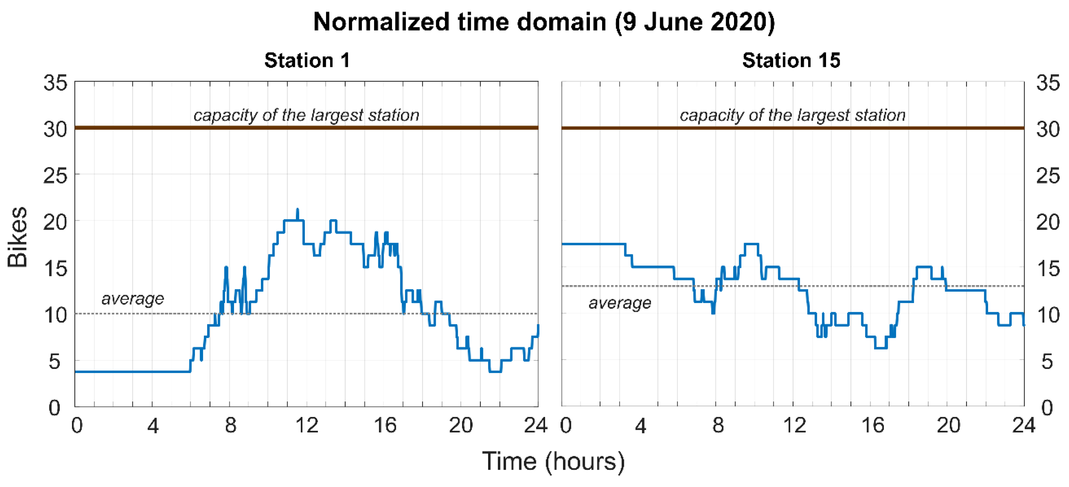
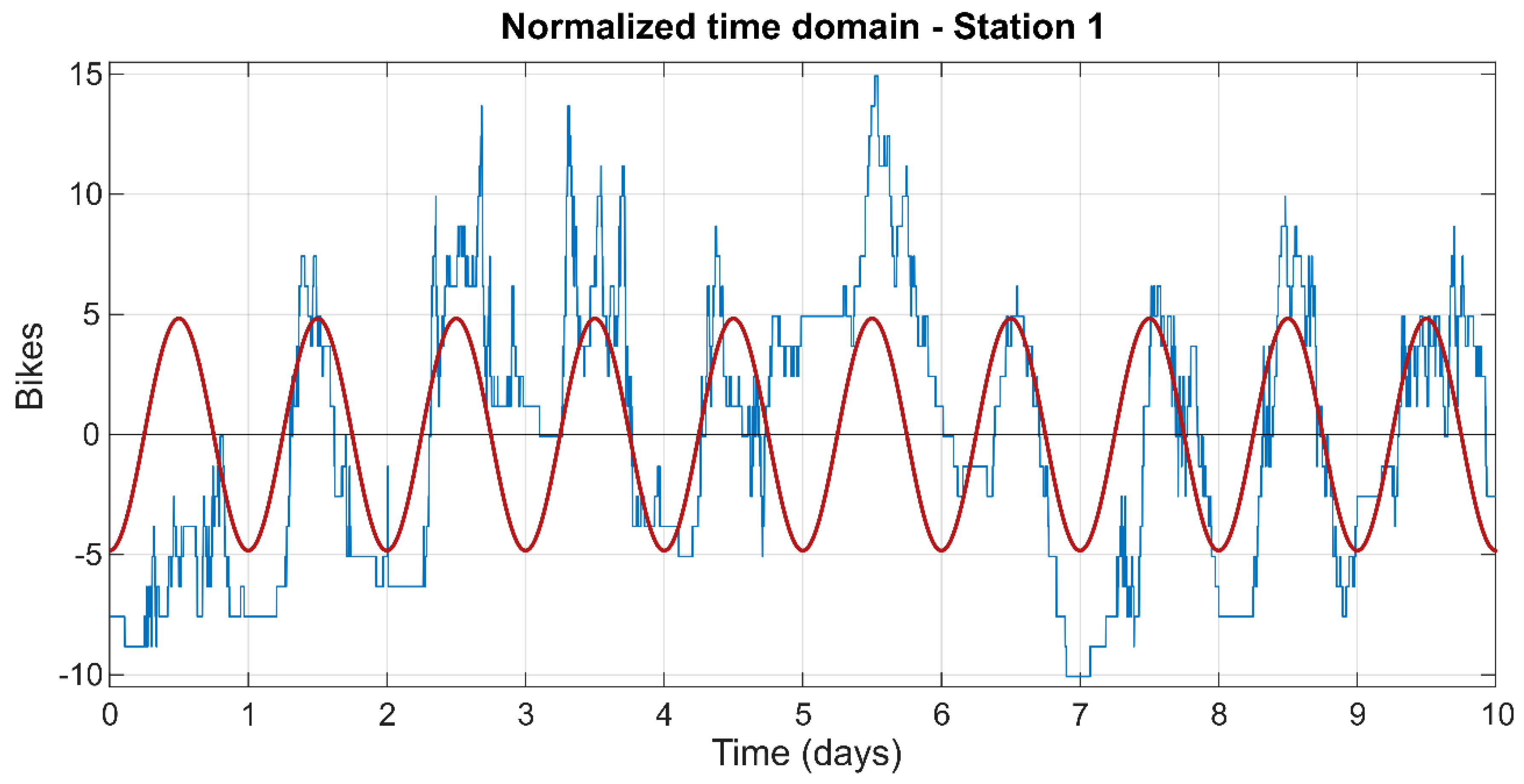
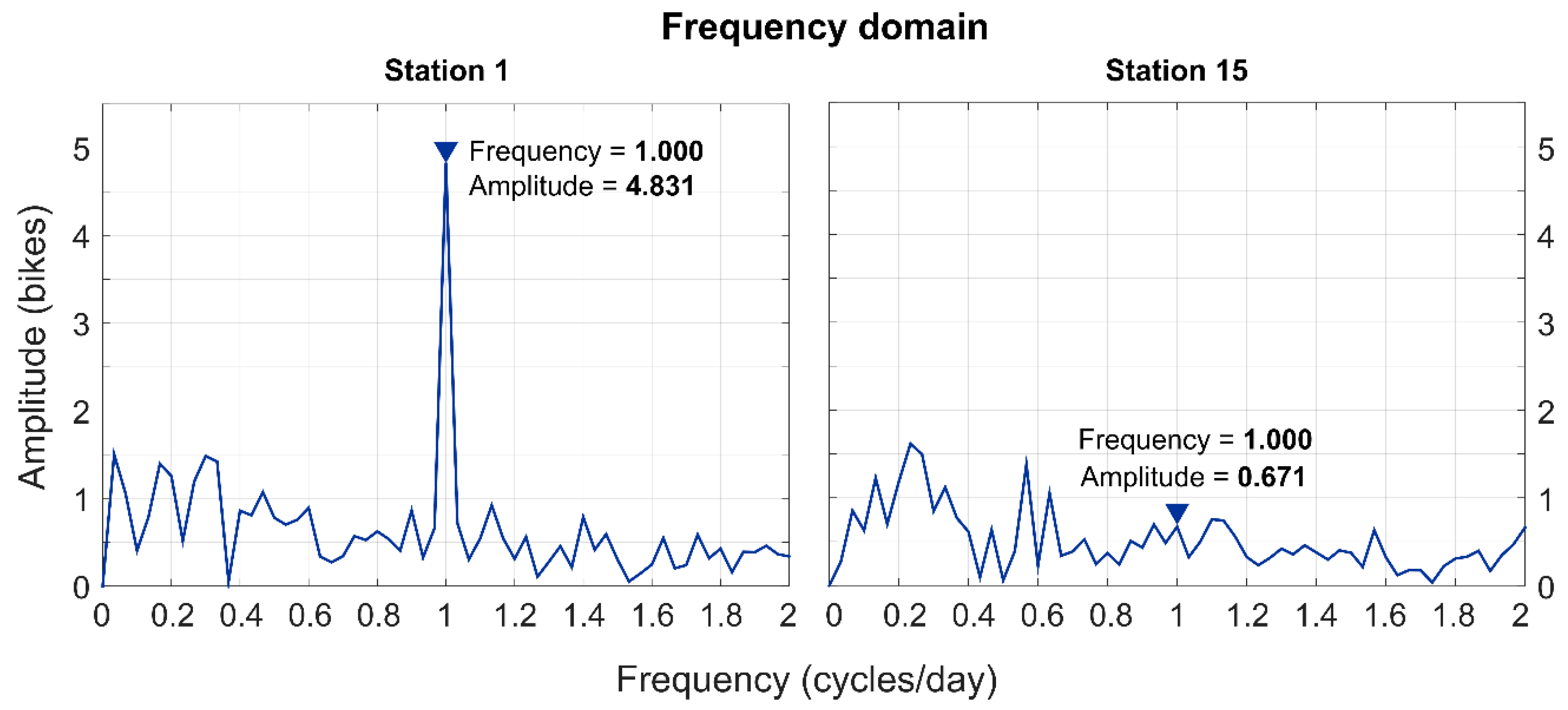
- Station daily amplitude: The station daily amplitude is a way to express the daily variation of the number of bicycles in each station. A higher value (higher amplitude) corresponds to a station that is more regularly used throughout the day. We suggest calculating the amplitude of each station using the fast Fourier transform [44]. Fast Fourier transforms are mathematical calculations that convert a domain waveform (amplitude versus time) into a series of discrete waves in the frequency domain. The daily amplitude for each station can be calculated starting from the bicycle variations (usage trends) in ΔT, obtaining their frequency domain using the fast Fourier transform, and assessing the (daily) amplitude value for frequency (cycles/day) = 1.
- Station prevalence: This indicator is a proxy for the share of bicycle trips that start (departure prevalence) or end (arrival prevalence) in each station.Given n BSS stations in the system, we count the number of trips starting in each stations si (picked-up bicycles) during Δt. Then, the stations are ordered from the one that originates more trips (assigning it a score equal to n) to the one that originates less trips (score = 1). The scores are assigned progressively, i.e., the second one in the list has n-1, the third one n-2, and so forth. This process is repeated for every day Δt in the timeframe ΔT of the analysis (since every station may show a different behavior according to Δt), and the daily scores assigned to each station si are summed. From these final scores, an average daily value is calculated, dividing the total score assigned to each station for the days Δt included in ΔT.This is the station prevalence calculated for the departures from each station (departure prevalence); the same reasoning can be applied looking at the arrivals (i.e., repeating the calculations for the number of bicycles dropped off in each station during Δt and then obtaining the average arrival prevalence in ΔT).
- Station attractiveness: attractiveness is understood as a way to assess how appealing the station is for BSS users compared to the other stations in the network. More specifically, we propose to distinguish an active attractiveness from a passive one, considering the trips that connect each BSS station with the other stations in the network. The unit of these indicators is km/day, associated with each station.To calculate the active station attractiveness, we compute how many trips start in the origin station si in ΔT, and we multiply each trip for the kilometers (real network distance, shortest path) necessary to reach the destination station. Then, this value is divided according to how many days are included in ΔT, to obtain an average daily value (km/day).The same (opposite) reasoning is applied to calculate the passive station attractiveness, i.e., how many trips have their destination in si in ΔT, computing again an average daily value (km/day).Note that round trips (that is, those trips having both origin and destination in si) should not be included in the calculations.
3. Case Study: Malmöbybike
3.1. Context Description and Related Variables
3.2. BSS Data Description and Preparation
3.3. Specification of Inputs and Outputs
3.4. Inputs, Outputs, and Station Selection
4. Results and Discussion
4.1. The Efficient BSS Stations
4.2. The Medium Efficient BSS Stations
4.3. The Least Efficient BSS Stations
5. Conclusions
Author Contributions
Funding
Institutional Review Board Statement
Informed Consent Statement
Data Availability Statement
Acknowledgments
Conflicts of Interest
References
- Cardenas, I.D.; Dewulf, W.; Vanelslander, T.; Smet, C.; Beckers, J. The E-Commerce Parcel Delivery Market and the Implications of Home B2C Deliveries Vs Pick-Up Points. Int. J. Transp. Econ. 2017, 44. [Google Scholar] [CrossRef]
- Hickman, R.; Vecia, G. Discourses, Travel Behaviour and the “Last Mile” in London. Available online: https://www.ingentaconnect.com/content/alex/benv/2016/00000042/00000004/art00003;jsessionid=ouwsa66uvkmd.x-ic-live-02 (accessed on 4 April 2019).
- Pal, A.; Zhang, Y. Free-Floating Bike Sharing: Solving Real-Life Large-Scale Static Rebalancing Problems-ScienceDirect. Available online: https://www.sciencedirect.com/science/article/pii/S0968090X17300992 (accessed on 26 March 2019).
- Kabak, M.; Erbaş, M.; Çetinkaya, C.; Özceylan, E. A GIS-Based MCDM Approach for the Evaluation of Bike-Share Stations. J. Clean. Prod. 2018, 201, 49–60. [Google Scholar] [CrossRef]
- Nikitas, A.; Wallgren, P.; Rexfelt, O. The Paradox of Public Acceptance of Bike Sharing in Gothenburg. Proc. Inst. Civ. Eng. Sustain. 2015, 169, 101–113. [Google Scholar] [CrossRef]
- Lånecyklar, S.; Lånecyklar, S. Available online: https://goteborg.se/wps/portal?uri=gbglnk%3agbg.page.1edf2db0-9d4c-4aa8-9fff-86cd711a0541 (accessed on 10 January 2021).
- LinBike. Linköpings Elcykelpool. Available online: https://linbike.se (accessed on 10 January 2021).
- Sveriges Första Regionala Hyrcykelsystem. Available online: /regional-utveckling/samhallsplanering-och-infrastruktur/hallbara-transporter/hyrcykelsystem (accessed on 10 January 2021).
- Macioszek, E.; Świerk, P.; Kurek, A. The Bike-Sharing System as an Element of Enhancing Sustainable Mobility—A Case Study Based on a City in Poland. Sustainability 2020, 12, 3285. [Google Scholar] [CrossRef]
- Song, M.; Wang, K.; Zhang, Y.; Li, M.; Qi, H. Impact Evaluation of Bike-Sharing on Bicycling Accessibility. Sustainability 2020, 12, 6124. [Google Scholar] [CrossRef]
- Hyland, M.; Hong, Z.; de Farias Pinto, H.K.R.; Chen, Y. Hybrid Cluster-Regression Approach to Model Bikeshare Station Usage. Transp. Res. Part A Policy Pract. 2018, 115, 71–89. [Google Scholar] [CrossRef]
- Li, A.; Zhao, P.; He, H.; Axhausen, K.W. Understanding the Variations of Micro-Mobility Behavior before and during COVID-19 Pandemic Period; IVT, ETH Zurich: Zurich, Switzerland, 2020; Volume 1547. [Google Scholar]
- Nikiforiadis, A.; Ayfantopoulou, G.; Stamelou, A. Assessing the Impact of COVID-19 on Bike-Sharing Usage: The Case of Thessaloniki, Greece. Sustainability 2020, 12, 8215. [Google Scholar] [CrossRef]
- Henriksson, M.; Wallsten, A. Succeeding without Success: Demonstrating a Residential Bicycle Sharing System in Sweden. Transp. Res. Interdiscip. Perspect. 2020, 8, 100271. [Google Scholar] [CrossRef]
- Nikitas, A. Understanding Bike-Sharing Acceptability and Expected Usage Patterns in the Context of a Small City Novel to the Concept: A Story of ‘Greek Drama’. Transp. Res. Part F Traffic Psychol. Behav. 2018, 56, 306–321. [Google Scholar] [CrossRef]
- Nikitas, A. How to Save Bike-Sharing: An Evidence-Based Survival Toolkit for Policy-Makers and Mobility Providers. Sustainability 2019, 11, 3206. [Google Scholar] [CrossRef]
- Liu, J.; Li, Q.; Qu, M.; Chen, W.; Yang, J.; Xiong, H.; Zhong, H.; Fu, Y. Station Site Optimization in Bike Sharing Systems. In Proceedings of the 2015 IEEE International Conference on Data Mining, Atlantic City, NJ, USA, 14–17 November 2015; pp. 883–888. [Google Scholar]
- Eren, E.; Uz, V.E. A Review on Bike-Sharing: The Factors Affecting Bike-Sharing Demand. Sustain. Cities Soc. 2020, 54, 101882. [Google Scholar] [CrossRef]
- Nogal, M.; Jiménez, P. Attractiveness of Bike-Sharing Stations from a Multi-Modal Perspective: The Role of Objective and Subjective Features. Sustainability 2020, 12, 9062. [Google Scholar] [CrossRef]
- Chen, E.; Ye, Z. Identifying the Nonlinear Relationship between Free-Floating Bike Sharing Usage and Built Environment. J. Clean. Prod. 2021, 280, 124281. [Google Scholar] [CrossRef]
- Hong, J.; Tamakloe, R.; Tak, J.; Park, D. Two-Stage Double Bootstrap Data Envelopment Analysis for Efficiency Evaluation of Shared-Bicycle Stations in Urban Cities. Transp. Res. Rec. 2020, 2674, 211–224. [Google Scholar] [CrossRef]
- Charnes, A.; Cooper, W.; Lewin, A.Y.; Seiford, L.M. Data Envelopment Analysis Theory, Methodology and Applications. J. Oper. Res. Soc. 1997, 48, 332–333. [Google Scholar] [CrossRef]
- Mariz, F.B.; Almeida, M.R.; Aloise, D. A Review of Dynamic Data Envelopment Analysis: State of the Art and Applications. Int. Trans. Oper. Res. 2018, 25, 469–505. [Google Scholar] [CrossRef]
- Markovits-Somogyi, R. Measuring Efficiency in Transport: The State of the Art of Applying Data Envelopment Analysis. Transport 2011, 26, 11–19. [Google Scholar] [CrossRef]
- Cavaignac, L.; Petiot, R. A Quarter Century of Data Envelopment Analysis Applied to the Transport Sector: A Bibliometric Analysis. Socio Econ. Plan. Sci. 2017, 57, 84–96. [Google Scholar] [CrossRef]
- Cheng, M.; Wei, W. An AHP-DEA Approach of the Bike-Sharing Spots Selection Problem in the Free-Floating Bike-Sharing System. Discret. Dyn. Nat. Soc. 2020, 2020. [Google Scholar] [CrossRef]
- Dyson, R.G.; Allen, R.; Camanho, A.S.; Podinovski, V.V.; Sarrico, C.S.; Shale, E.A. Pitfalls and Protocols in DEA. Eur. J. Oper. Res. 2001, 132, 245–259. [Google Scholar] [CrossRef]
- Ewing, R.; Cervero, R. Travel and the Built Environment. J. Am. Plan. Assoc. 2010, 76, 265–294. [Google Scholar] [CrossRef]
- Croci, E.; Rossi, D. Optimizing the Position of Bike Sharing Stations. The Milan Case; Social Science Research Network: Rochester, NY, USA, 2014. [Google Scholar]
- NACTO Urban Street Design Guide. Available online: https://nacto.org/publication/urban-street-design-guide (accessed on 11 January 2021).
- The Bike Share Planning Guide. Available online: https://www.itdp.org/who-we-are/for-the-press/the-bike-share-planning-guide (accessed on 11 January 2021).
- Bachand-Marleau, J.; Larsen, J.; El-Geneidy, A. Much-Anticipated Marriage of Cycling and Transit: How Will It Work? Transp. Res. Rec. J. Transp. Res. Board 2011, 109–117. [Google Scholar] [CrossRef]
- NACTO Walkable Station Spacing Is Key to Successful, Equitable Bike Share. Available online: https://nacto.org/2015/04/28/walkable-station-spacing-is-key-to-successful-equitable-bike-share (accessed on 11 January 2021).
- Schoner, J.E.; Levinson, D.M. The Missing Link: Bicycle Infrastructure Networks and Ridership in 74 US Cities. Transportation 2014, 41, 1187–1204. [Google Scholar] [CrossRef]
- Dill, J.; Voros, K. Factors Affecting Bicycling Demand: Initial Survey Findings from the Portland, Oregon, Region. Transp. Res. Rec. J. Transp. Res. Board 2007, 9–17. [Google Scholar] [CrossRef]
- Hamidi, Z.; Zhao, C. Shaping Sustainable Travel Behaviour: Attitude, Skills, and Access All Matter. Transp. Res. Part D Transp. Environ. 2020, 88, 102566. [Google Scholar] [CrossRef]
- Yang, M.; Zacharias, J. Potential for Revival of the Bicycle in Beijing. Int. J. Sustain. Transp. 2016, 10, 517–527. [Google Scholar] [CrossRef]
- Shaheen, S.; Cohen, A.; Martin, E. Public Bikesharing in North America. Transp. Res. Rec. J. Transp. Res. Board 2013, 2387, 83–92. [Google Scholar] [CrossRef]
- Caggiani, L.; Colovic, A.; Ottomanelli, M. An Equality-Based Model for Bike-Sharing Stations Location in Bicycle-Public Transport Multimodal Mobility. Transp. Res. Part A Policy Pract. 2020, 140, 251–265. [Google Scholar] [CrossRef]
- Fishman, E.; Washington, S.; Haworth, N. Barriers and Facilitators to Public Bicycle Scheme Use: A Qualitative Approach. Transp. Res. Part F Traffic Psychol. Behav. 2012, 15, 686–698. [Google Scholar] [CrossRef]
- Zhao, C.; Nielsen, T.A.S.; Olafsson, A.S.; Carstensen, T.A.; Meng, X. Urban Form, Demographic and Socio-Economic Correlates of Walking, Cycling, and e-Biking: Evidence from Eight Neighborhoods in Beijing. Transp. Policy 2018. [Google Scholar] [CrossRef]
- Lu, W.; Scott, D.M.; Dalumpines, R. Understanding Bike Share Cyclist Route Choice Using GPS Data: Comparing Dominant Routes and Shortest Paths. J. Transp. Geogr. 2018, 71, 172–181. [Google Scholar] [CrossRef]
- Maas, S.; Nikolaou, P.; Attard, M.; Dimitriou, L. Examining Spatio-Temporal Trip Patterns of Bicycle Sharing Systems in Southern European Island Cities. Res. Transp. Econ. 2020, 100992. [Google Scholar] [CrossRef]
- Cerna, M.; Harvey, A.F. The Fundamentals of FFT-Based Signal Analysis and Measurement; National Instruments: Batu Maung, Malaysia, 2000. [Google Scholar]
- Statistics Sweden Population by Region, Marital Status, Age and Sex. Year 1968–2019. Available online: https://www.statistikdatabasen.scb.se/pxweb/en/ssd (accessed on 31 December 2020).
- Malmöstad. Cykelbanor och Bilvägar. Available online: http://miljobarometern.malmo.se/trafik/cykling/cykelbanor-och-bilvagar (accessed on 6 January 2021).
- Region Skåne Resevaneundersökning 2018 Interaktiv Webbplats. Available online: https://utveckling.skane.se/publikationer/rapporter-analyser-och-prognoser/resvaneundersokning-i-skane (accessed on 31 December 2020).
- Lantmäteriet GSD-Property Map (SWEREF99TM). Available online: https://www.lantmateriet.se/globalassets/kartor-och-geografisk-information/kartor/e_fastshmi.pdf (accessed on 30 December 2020).
- Trafikverket NVDB GCM-Vägtyp. Available online: https://www.trafikverket.se/TrvSeFiler/Dataproduktspecifikationer/V%C3%A4gdataprodukter/DPS_E-G/1054gcm-vagtyp.pdf (accessed on 30 December 2020).
- Hamidi, Z.; Camporeale, R.; Caggiani, L. Inequalities in Access to Bike-and-Ride Opportunities: Findings for the City of Malmö. Transp. Res. Part A Policy Pract. 2019, 130, 673–688. [Google Scholar] [CrossRef]
- Clearchannel Clearchannel.Se. Available online: https://www.clearchannel.se (accessed on 31 December 2020).
- Average Weather in June in Malmö, Sweden-Weather Spark. Available online: https://weatherspark.com/m/76106/6/Average-Weather-in-June-in-Malm%C3%B6-Sweden (accessed on 31 December 2020).
- Malmö by Bike. Available online: https://www.malmobybike.se/en/info/about-malmo-by-bike (accessed on 31 December 2020).
- Kabra, A.; Belavina, E.; Girotra, K. Bike-Share Systems: Accessibility and Availability. Manag. Sci. 2020, 66, 3803–3824. [Google Scholar] [CrossRef]
- Sarkis, J. Preparing your data for DEA. In Modeling Data Irregularities and Structural Complexities in Data Envelopment Analysis; Springer: Berlin/Heidelberg, Germany, 2007; pp. 305–320. [Google Scholar]
- Trafikverket Geodata-Lantmäteriet, Dataproduktspecifikation-Hållplats. Available online: https://www.trafikverket.se/TrvSeFiler/Dataproduktspecifikationer/V%C3%A4gdataprodukter/DPS_H-K/1011Hallplats.pdf (accessed on 30 December 2020).
- Statistics Sweden Population Statistics (SWEREF99TM). Available online: https://www.scb.se/en/finding-statistics/statistics-by-subject-area/population/population-composition/population-statistics/ (accessed on 30 December 2020).
- Statistics Sweden Labour Market and Education Statistics (SWEREF99TM). Available online: http://www.scb.se/en/finding-statistics/statistics-by-subject-area/labour-market (accessed on 30 December 2020).
- Statistics Sweden Income Statistics (SWEREF99TM). Available online: http://www.scb.se/en/finding-statistics/statistics-by-subject-area/household-finances/income-and-income-distribution/income-and-tax-statistics (accessed on 30 December 2020).
- Boyd, T.; Docken, G.; Ruggiero, J. Outliers in data envelopment analysis. J. Cent. Cathedra 2016, 9, 168–183. [Google Scholar] [CrossRef]
- Huang, H.; Liao, W. A Co-Plot-Based Efficiency Measurement to Commercial Banks. JSW 2012, 7, 2247–2251. [Google Scholar] [CrossRef][Green Version]
- Adler, N.; Raveh, A. Presenting DEA Graphically. Omega 2008, 36, 715–729. [Google Scholar] [CrossRef]
- Nath, P.; Mukherjee, A.; Pal, M.N. Identification of Linkage between Strategic Group and Performance of Indian Commercial Banks: A Combined Approach Using DEA and Co-Plot. Int. J. Digit. Account. Res. 2001, 1, 125–152. [Google Scholar] [CrossRef][Green Version]
- Atilgan, Y.K. Robust Coplot Analysis. Commun. Stat. Simul. Comput. 2016, 45, 1763–1775. [Google Scholar] [CrossRef]
- Atilgan, Y.K.; Atilgan, E.L. RobCoP: A Matlab Package for Robust CoPlot Analysis. Open J. Stat. 2017, 7, 23–35. [Google Scholar] [CrossRef]
- Kuljanin, J.; Kalić, M.; Caggiani, L.; Ottomanelli, M. A Comparative Efficiency and Productivity Analysis: Implication to Airlines Located in Central and South-East Europe. J. Air Transp. Manag. 2019, 78, 152–163. [Google Scholar] [CrossRef]
- Bravata, D.M.; Shojania, K.G.; Olkin, I.; Raveh, A. CoPlot: A Tool for Visualizing Multivariate Data in Medicine. Stat. Med. 2008, 27, 2234–2247. [Google Scholar] [CrossRef] [PubMed]
- Krzanowski, W.J.; Dillon, W.R.; Goldstein, M. Multivariate Analysis-Methods and Applications. Biometrics 1986, 42, 222. [Google Scholar] [CrossRef]
- Borg, I.; Groenen, P.J. Modern Multidimensional Scaling: Theory and Applications; Springer Science & Business Media: Berlin/Heidelberg, Germany, 2005. [Google Scholar]
- Cox, M.A.A.; Cox, T.F. Multidimensional Scaling. In Handbook of Data Visualization; Chen, C., Härdle, W., Unwin, A., Eds.; Springer: Berlin/Heidelberg, Germany, 2008; pp. 315–347. [Google Scholar]
- Kruskal, J.B. Multidimensional Scaling by Optimizing Goodness of Fit to a Nonmetric Hypothesis. Psychometrika 1964, 29, 1–27. [Google Scholar] [CrossRef]
- Caulfield, B.; Brick, E.; McCarthy, O.T. Determining Bicycle Infrastructure Preferences-A Case Study of Dublin. Transp. Res. Part D Transp. Environ. 2012, 17, 413–417. [Google Scholar] [CrossRef]
- Mateo-Babiano, I.; Bean, R.; Corcoran, J.; Pojani, D. How Does Our Natural and Built Environment Affect the Use of Bicycle Sharing? Transp. Res. Part A Policy Pract. 2016, 94, 295–307. [Google Scholar] [CrossRef]
- Kim, D.; Shin, H.; Im, H.; Park, J. Factors Influencing Travel Behaviors in Bikesharing. Available online: https://nacto.org/wp-content/uploads/2012/02/Factors-Influencing-Travel-Behaviors-in-Bikesharing-Kim-et-al-12-1310.pdf (accessed on 30 December 2020).
- McBain, C.; Caulfield, B. An Analysis of the Factors Influencing Journey Time Variation in the Cork Public Bike System. Sustain. Cities Soc. 2018, 42, 641–649. [Google Scholar] [CrossRef]
- Kaltenbrunner, A.; Meza, R.; Grivolla, J.; Codina, J.; Banchs, R. Urban Cycles and Mobility Patterns: Exploring and Predicting Trends in a Bicycle-Based Public Transport System. Pervasive Mob. Comput. 2010, 6, 455–466. [Google Scholar] [CrossRef]
- Ewing, R.; Cervero, R. Travel and the Built Environment: A Synthesis. Transp. Res. Rec. J. Transp. Res. Board 2001, 1780, 87–114. [Google Scholar] [CrossRef]
- El-Assi, W.; Salah Mahmoud, M.; Nurul Habib, K. Effects of Built Environment and Weather on Bike Sharing Demand: A Station Level Analysis of Commercial Bike Sharing in Toronto. Transportation 2017, 44, 589–613. [Google Scholar] [CrossRef]
- Maurer, L.K. Feasibility Study for a Bicycle Sharing Program in Sacramento, California. Available online: https://nacto.org/wp-content/uploads/2012/02/Feasibility-Study-for-a-Bicycle-Sharing-Program-in-Sacramento-California-Maurer-12-4431.pdf (accessed on 30 December 2020).


| Input Variables | Rationality and Description of the Variables |
|---|---|
| BSS Station Related Variables | |
| Station age | The variable is relevant for more complex/old systems, particularly if the system has been developed during several stages and groups of stations have been added at different points in time. It can be measured according to the age context of the stations. |
| Visibility of stations | Visibility of the stations should consider if they are placed next to public transport, or in green areas (i.e., partially hidden by trees/bushes), or in a well-lit environment [29,30,31]. It can be measured taking into account the involved elements, i.e., by assessing the distance to the bus stops/metro stations, and/or the area of the bushes around the stations, etc. |
| Density of BSS station | The proximity of BSS stations to each other contribute to the increasing demand for BSS services [32,33]. Different buffers have been suggested for effective BSSs in various contexts [18]. |
| Built environment variables | |
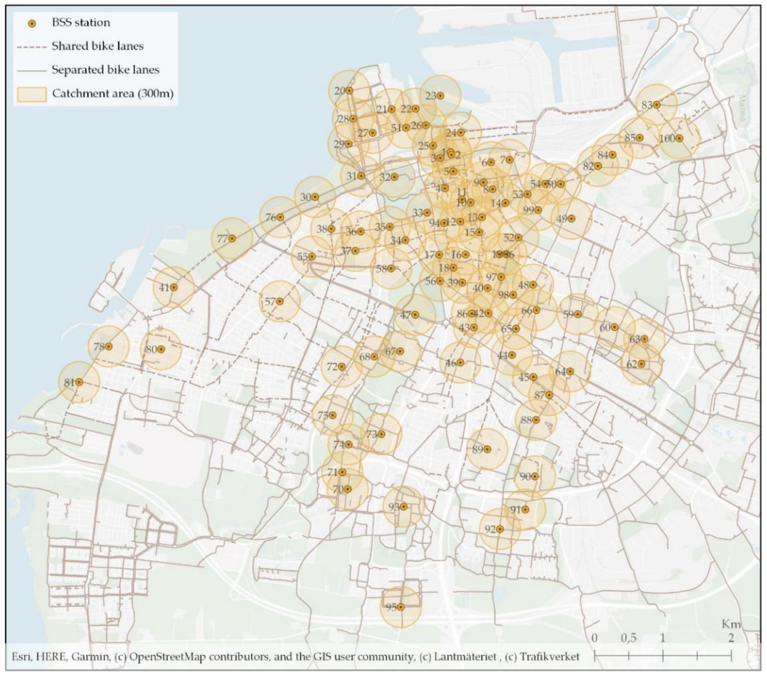
| Bicycle infrastructure | Increasing the usage of bicycles requires good bicycle infrastructure [34]. The proximity of BSS stations to the cycling infrastructure impacts the motivation of cycling [35]. This variable can be measured computing the total length of bike lanes within the catchment area of each station, possibly weighted by the type of the bike lanes (e.g., separated paths versus paths shared with traffic). |
| Street connectivity | Street connectivity reflects the level of infrastructure and traffic safety in the network surrounding a BSS station [36,37]. The variable can be applied or not according to the context, it can be measured calculating the number of intersections and the density of the road network in the area. |
| Public transport (PT) impact factors | BSS likely promotes the mode share of public transport by serving as a feeder mode for PT [38,39], and vice versa, the provision of the PT service can impact the usage of BSS. Three dimensions related to the public transport can be measured: (1) distance to the PT stations (i.e., bus stops, railways stations); (2) level of provision, which can be measured by the number of stops and stations, number of bus lines, ride frequency; (3) price scheme and approach for accessing to PT and BSS services, e.g., using a smart card for accessing to both services with a fair price is likely to increase the usage of BSS service [28,36,40,41]. |
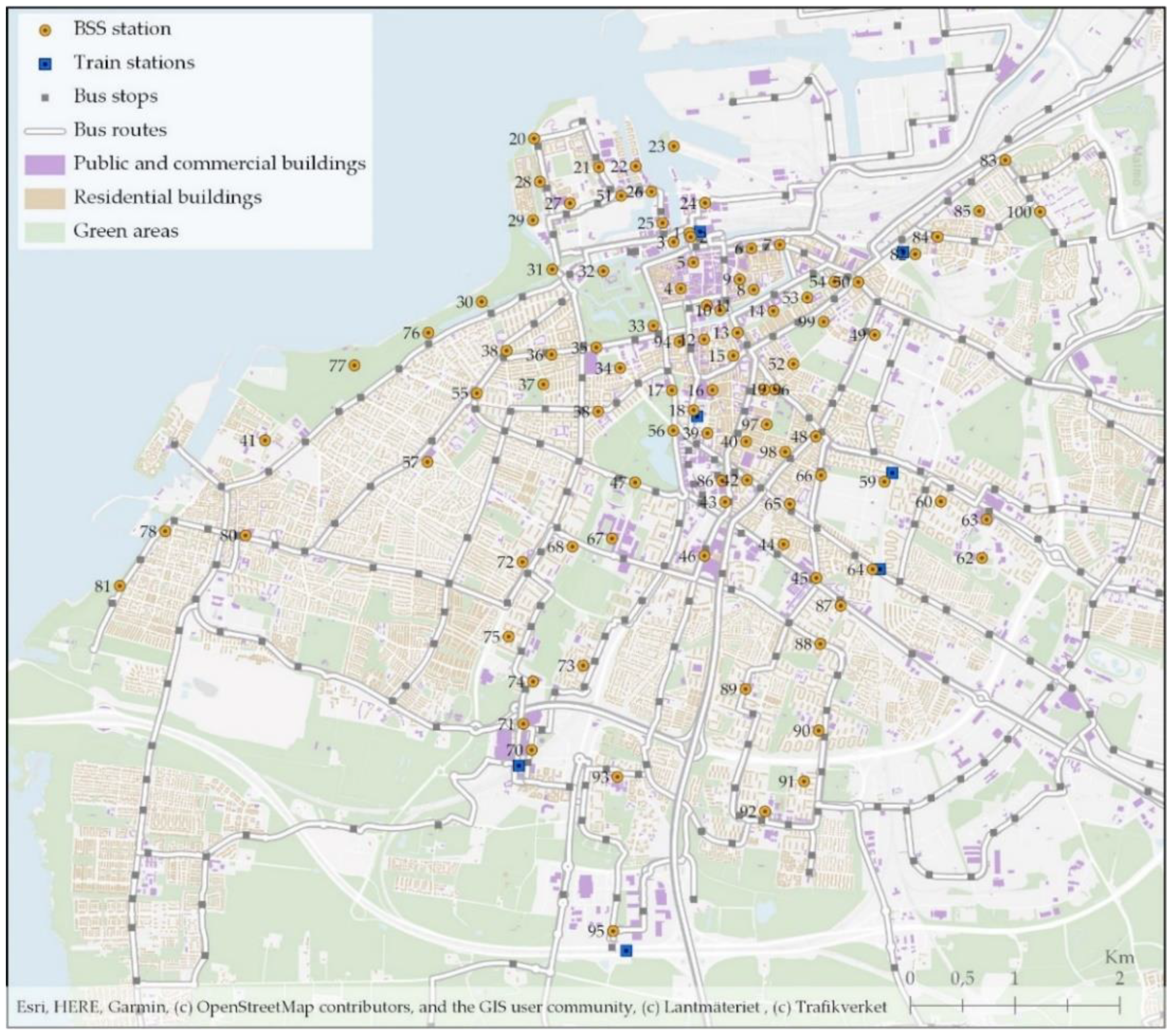
| Land Use | Land use impacts the demand for trips and affects the choice of travel modes. Residential areas, public and commercial areas, green areas in the city and outskirt, and mixed level of land use are the main parameters for measuring the impact of land use [28,41]. |
| Slope (morphology of the territory) | Slope is one of the main barriers for motivating cyclists to cycle and it strongly affects bicycle usage [18]. It can be measured by assessing the level of slope in specific streets, and the portion of the streets with a certain slope within the city and catchment area [42]. It should be included/considered as a parameter in the general model formulation especially for those cities that have hilly topographies. |
| Population related variables | |
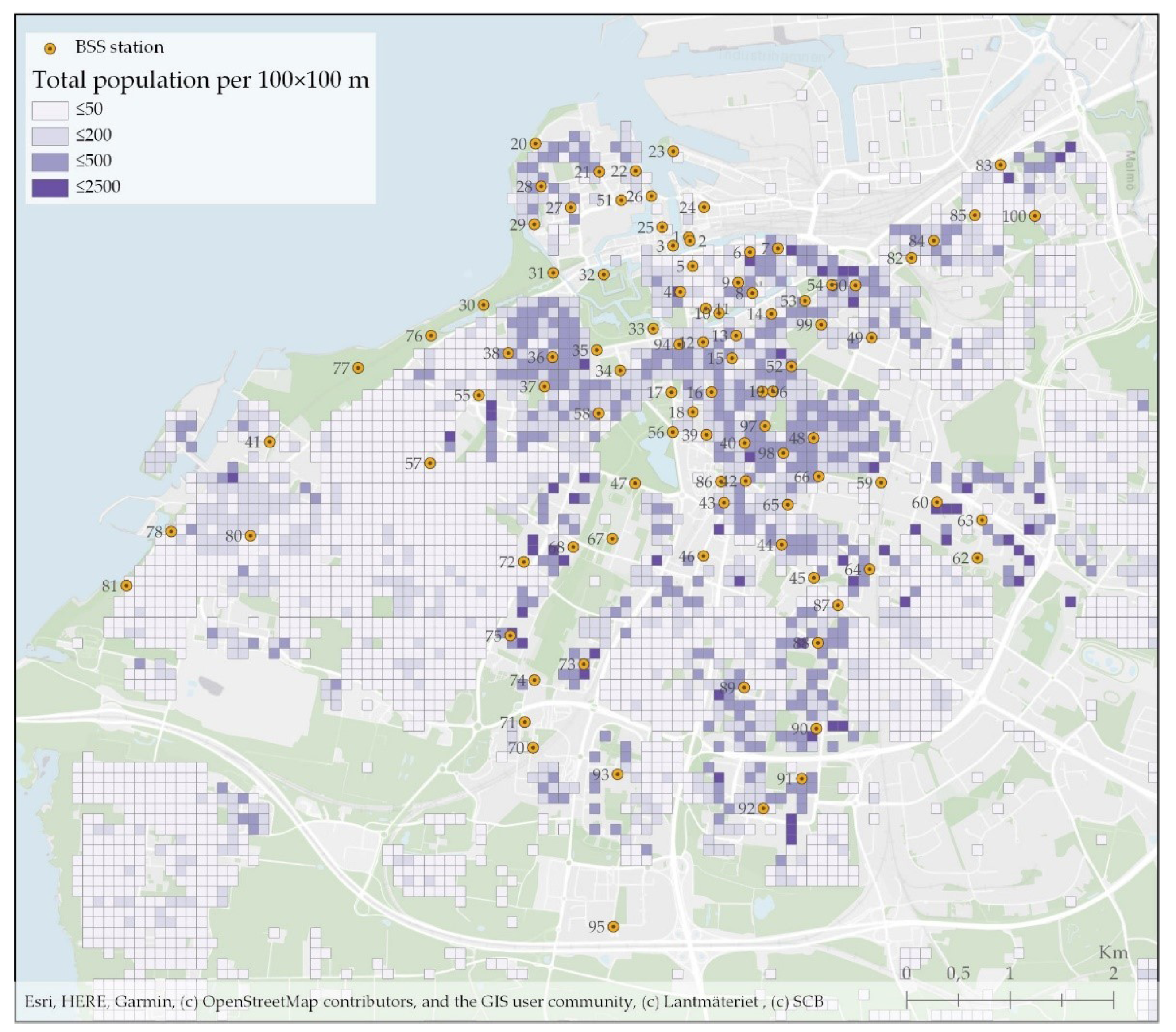
| Population size | Population size in the catchment area is an important factor that influences the usage of the BSS service [43]. It can be measured by calculating the number of individuals residing in the catchment area. |
| Sociodemographic | Age, gender, education, income, employment, ownership of transit mode are the individual factors that most impact the travel behavior [18,41,43]; therefore, these are the parameters within the catchment area suggested to be measured. |
| Input Variables | Description of the Variables | DEA Notation |
|---|---|---|
| BSS Station Related Variables | ||
| Density of BSS stations | Number of the BSS stations within 1 km radius from each BSS station | I1 Density of BSS stations (within 1 km) |
| Built environmental variables (within the catchment area) | ||
| Land use | The area of each land use category. Three types of land use are calculated: residential; public and commercial; green areas [48]. | I2 Green areas (km2) I3 Residential (km2) I4 Public + Commercial (km2) |
| Bicycle infrastructure | The total length of bike lanes. We computed separated bike lanes and shared bike lanes. Separated bike lanes refer to the designated road space clearly defined by signs and regulations that space should be only used for cycling; shared bike lanes are the road spaces shared with pedestrian or cars but recommended for cycling in the interest of creating a more continuous cycling network across the city [49]. | I5 Separated bike lanes (m) I6 Shared bike lanes (m) |
| Public transport impact factors | The number of tracks/bus lines passing by each station/bus stop, to have a proxy of the actual connectivity granted by the public transport system [56]. | I7 Number of tracks I8 Number of bus lines |
| Population related variables (within the catchment area) | ||
| Population size | The average number of residents. Since each catchment area is delimited by a circle, and the population is available in a grid format, we calculated the portion of the area of each element of the grid (square) falling within the circle, and the corresponding share of population assuming a uniform population density in each element of the grid. Provided in grid format (2018), 100 × 100 m [57]. | I9 Population size |
| Age | Population aged 16–64, in grid format (2018), 250 × 250 m urban area, 1000 × 1000 m in suburban areas [57]. | I10 Population aged 16–64 |
| Employment | For the population aged 20–64 (only 2017), two categories of employment are measured: Employed, Unemployed [58]. | I11 Unemployed I12 Employed |
| Household disposable income (2018) | Household disposable income (2018) is measured in four levels: low, medium-low, medium-high, high. The indicator is adjusted considering the consumption units in a household meaning it accounts for different household compositions [59]. | I13 Income: low I14 Income: medium-low I15 Income medium-high I16 Income: high |
| Education | For the population aged 25–64 (2018), four levels of education are measured: Compulsory education, Upper secondary, Post-secondary, less than 3 years and Post-secondary, 3 years or longer, including graduate and postgraduate education [58]. | I17 Education: level 1 I18 Education: level 2 I19 Education: level 3 I20 Education: level 4 |
| I1 | I2 | I3 | I4 | I5 | I6 | I7 | I8 | I9 | I10 | |
|---|---|---|---|---|---|---|---|---|---|---|
| Mean | 12.07 | 0.04 | 34,054.29 | 29,626.77 | 1880.77 | 371.21 | 0.65 | 5.88 | 2610.06 | 1701.69 |
| Median | 11.00 | 0.03 | 31,174.89 | 21,718.77 | 1827.97 | 261.96 | 0.00 | 2.00 | 2480.00 | 1634.00 |
| Std. dev. | 7.31 | 0.04 | 23,024.89 | 26,015.10 | 861.93 | 394.64 | 2.12 | 8.19 | 1853.44 | 1226.74 |
| Minimum | 1.00 | 0.0001 | 1.00 | 42.47 | 1.00 | 1.00 | 0.0001 | 0.0001 | 1.00 | 30.00 |
| Maximum | 26.00 | 0.24 | 87,317.85 | 110,052.80 | 4468.33 | 1911.09 | 10.00 | 50.00 | 7292.00 | 5230.00 |
| I11 | I12 | I13 | I14 | I15 | I16 | I17 | I18 | I19 | I20 | |
| Mean | 566.44 | 1155.98 | 424.91 | 286.49 | 266.84 | 243.72 | 170.39 | 454.59 | 279.72 | 593.02 |
| Median | 533.50 | 1000.00 | 406.50 | 262.00 | 197.50 | 163.50 | 113.00 | 452.50 | 240.00 | 419.50 |
| Std. dev. | 429.96 | 862.35 | 329.60 | 215.67 | 216.59 | 207.98 | 164.89 | 307.23 | 209.39 | 505.34 |
| Minimum | 1.00 | 1.00 | 1.00 | 1.00 | 1.00 | 1.00 | 1.00 | 1.00 | 1.00 | 1.00 |
| Maximum | 1650.00 | 3451.00 | 1232.00 | 943.00 | 902.00 | 936.00 | 851.00 | 1108.00 | 845.00 | 1891.00 |
| Output Variables | DEA Notation | Mean | Median | Std. Dev. | Minimum | Maximum |
|---|---|---|---|---|---|---|
| Station daily amplitude | O1 | 2.01 | 1.54 | 1.57 | 0.12 | 6.70 |
| Station arrival prevalence | O2 | 54.07 | 55.08 | 24.99 | 11.77 | 86.23 |
| Station departure prevalence | O3 | 54.06 | 55.85 | 25.07 | 10.03 | 88.07 |
| Station passive attractiveness | O4 | 45.82 | 36.19 | 30.05 | 5.85 | 122.65 |
| Station active attractiveness | O5 | 45.82 | 38.06 | 29.34 | 6.40 | 122.24 |
Publisher’s Note: MDPI stays neutral with regard to jurisdictional claims in published maps and institutional affiliations. |
© 2021 by the authors. Licensee MDPI, Basel, Switzerland. This article is an open access article distributed under the terms and conditions of the Creative Commons Attribution (CC BY) license (http://creativecommons.org/licenses/by/4.0/).
Share and Cite
Caggiani, L.; Camporeale, R.; Hamidi, Z.; Zhao, C. Evaluating the Efficiency of Bike-Sharing Stations with Data Envelopment Analysis. Sustainability 2021, 13, 881. https://doi.org/10.3390/su13020881
Caggiani L, Camporeale R, Hamidi Z, Zhao C. Evaluating the Efficiency of Bike-Sharing Stations with Data Envelopment Analysis. Sustainability. 2021; 13(2):881. https://doi.org/10.3390/su13020881
Chicago/Turabian StyleCaggiani, Leonardo, Rosalia Camporeale, Zahra Hamidi, and Chunli Zhao. 2021. "Evaluating the Efficiency of Bike-Sharing Stations with Data Envelopment Analysis" Sustainability 13, no. 2: 881. https://doi.org/10.3390/su13020881
APA StyleCaggiani, L., Camporeale, R., Hamidi, Z., & Zhao, C. (2021). Evaluating the Efficiency of Bike-Sharing Stations with Data Envelopment Analysis. Sustainability, 13(2), 881. https://doi.org/10.3390/su13020881