Article

Day-Ahead Electric Load Forecast for a Ghanaian Health Facility Using Different Algorithms

by
Samer Chaaraoui
1,*,
Matthias Bebber
1,
Stefanie Meilinger
1,
Silvan Rummeny
2,
Thorsten Schneiders
2,
Windmanagda Sawadogo
3 and
Harald Kunstmann
3,4
1
International Centre for Sustainable Development (IZNE), University of Applied Sciences Bonn-Rhein-Sieg, 53757 Sankt Augustin, Germany
2
Cologne Institute for Renewable Energy (CIRE), University of Applied Sciences Cologne, 50679 Cologne, Germany
3
Institute of Geography, University of Augsburg, 86159 Augsburg, Germany
4
Campus Alpin, Institute of Meteorology and Climate Research (IMK-IFU), Karlsruhe Institute of Technology (KIT), 82467 Garmisch-Partenkirchen, Germany
*
Author to whom correspondence should be addressed.
Energies 2021, 14(2), 409; https://doi.org/10.3390/en14020409
Submission received: 30 November 2020 / Revised: 7 January 2021 / Accepted: 9 January 2021 / Published: 13 January 2021
(This article belongs to the Special Issue Artificial Intelligence Technologies for Electric Power Systems)

Abstract

:
Ghana suffers from frequent power outages, which can be compensated by off-grid energy solutions. Photovoltaic-hybrid systems become more and more important for rural electrification due to their potential to offer a clean and cost-effective energy supply. However, uncertainties related to the prediction of electrical loads and solar irradiance result in inefficient system control and can lead to an unstable electricity supply, which is vital for the high reliability required for applications within the health sector. Model predictive control (MPC) algorithms present a viable option to tackle those uncertainties compared to rule-based methods, but strongly rely on the quality of the forecasts. This study tests and evaluates (a) a seasonal autoregressive integrated moving average (SARIMA) algorithm, (b) an incremental linear regression (ILR) algorithm, (c) a long short-term memory (LSTM) model, and (d) a customized statistical approach for electrical load forecasting on real load data of a Ghanaian health facility, considering initially limited knowledge of load and pattern changes through the implementation of incremental learning. The correlation of the electrical load with exogenous variables was determined to map out possible enhancements within the algorithms. Results show that all algorithms show high accuracies with a median normalized root mean square error (nRMSE) <0.1 and differing robustness towards load-shifting events, gradients, and noise. While the SARIMA algorithm and the linear regression model show extreme error outliers of nRMSE >1, methods via the LSTM model and the customized statistical approaches perform better with a median nRMSE of 0.061 and stable error distribution with a maximum nRMSE of <0.255. The conclusion of this study is a favoring towards the LSTM model and the statistical approach, with regard to MPC applications within photovoltaic-hybrid system solutions in the Ghanaian health sector.

1. Introduction

The electrical demand in sub-Saharan Africa is increasing due to rapid growth in population, which results in the highest increase in electrical demand worldwide. Although the population of those without electricity access decreased by 2.45% between 2013 and 2018, the electrification rate remains low at 45%. Furthermore, 80% of sub-Saharan African businesses suffer from an unreliable electricity supply, resulting from old power grid hardware and poor network management [1]. Ghana in particular is the regional leader in terms of electrification rates, but still suffers from low access in rural areas [2]. In addition, the Ghanaian energy sector suffers from high transmission and distribution losses of around 20%, while electricity prices are rising due to inflation and poor contracting with foreign power plant suppliers, resulting in a shift from a low electricity access and moderate affordability to a high electricity access and low affordability [3].
Implementation of renewable energy systems, such as decentralized photovoltaic (PV) and diesel hybrid systems, presents a viable option for an independent and a reliable electricity source in rural electrification scenarios. However, renewable energy systems represent a minority in the Ghanaian electricity generation mix with 0.03%, compared to hydro power with 31.97% and thermal power with 68% [4,5,6]. Consumers strongly rely on diesel generators to complement low electricity access rates and the poor reliability. On one hand, the health sector ensures a high reliability of their electrical supply through diesel generators compared to obtaining their electrical supply through the public grid. On the other hand, airborne carcinogens emitted by the diesel generators present a health risk for people inside, and in close vicinity of, the health facility [7,8].
Model predictive control (MPC) algorithms, which use load and solar radiation forecasts to optimize the dispatch of PV-diesel hybrid systems, have shown significant advantages compared to rule-based dispatch algorithms [9,10]. The results from Sachs et al. [9] indicate a decrease in the levelized cost of electricity (LCOE) by 6.8% with the proposed MPC algorithm compared to rule-based dispatch algorithms. An optimal control with complete knowledge of the future load and PV yield decreases the LCOE by 7.8% compared to rule-based algorithms. However, the performance of MPC algorithms highly relies on the forecasting algorithms accuracy. Sachs et al. [9] applied a seasonal autoregressive integrated moving average (SARIMA) algorithm to generate electricity demand and solar radiation forecasts. While the reduction of the LCOE through the implementation of a SARIMA forecasting algorithm shows improvements close to an optimal control of the system, it is difficult to derive the relative performance of the forecasting algorithm as results are given in absolute values and detailed information about the data used is not available. However, other publications analyzing the SARIMA algorithm for load forecasting purposes applied relative metrics as a measure for comparison and indicated good overall performance [11,12].
Moreover, Bozkurt et al. [12] show that the usage of artificial neural networks outperforms SARIMA-based algorithms, which is also observed in other publications using long short-term memory (LSTM) neural networks [13,14,15]. A method proposed by Steinebach et al. [16] presented a computationally simple algorithm, which generates forecasts through an incremental linear regression (ILR) method generated through a look-up table of gradients based on previous observations. In Bruno et al. [17], the authors used a hybrid forecasting method, which combines an autoregressive integrated moving average (ARIMA) algorithm, a neural network approach, and a seasonal trend decomposition method based on local regression lines defined as locally estimated scatterplot smoothing (LOESS). The hybrid forecasting method determines throughout its operation which algorithm and parametrization suits best after a predefined duration, allowing a certain plasticity towards load pattern changes throughout the operation time of the algorithm, which is also addressed in our study. The authors also point out the relevance of MPC applications with regard to the domestic, commercial, and industrial sector.
Maitanova et al. [18] developed a forecasting algorithm with regard to PV power forecasts based on publicly available data of the global horizontal irradiance using an LSTM approach with the integration of meteorological exogenous variables, and addressing the relevance of accurate forecasting for energy management systems, of which the MPC algorithm is one approach. However, Diagne et al. [19] addressed the forecasts’ temporal resolution and the forecast horizon, which determine if either SARIMA algorithms or artificial neural network approaches are more suitable for solar irradiance forecasts, while not specifying the kind of artificial neural network approach evaluated in the study.
This study aims to identify the most suitable forecasting algorithm regarding the characteristics of typical load curves of a Ghanaian health facility, analyzing the following methods.
  • SARIMA algorithm
  • ILR method
  • Neural networks with LSTM neurons
  • Custom statistical approach formulated throughout this research
The forecasting algorithms will be tested using load data from a medium-sized hospital in Southern Ghana, while using incremental learning to consider initially limited data availability which increments throughout the operation period of a fictional PV-hybrid system. The algorithms should therefore adapt to pattern changes, noise, and changing base load. Literature suggests sophisticated approaches, optimizing incremental learning algorithms to minimize computation resources for training, while showing proper plasticity towards high temporal variability in the data set [20,21,22,23]. However, the goal of this study is to identify the most suitable and accurate forecasting algorithm. Incremental learning will be implemented as simply as possible, just to take the incrementing data availability over the simulation period into account.
The integration of exogenous variables, the ambient temperature in particular, will be statistically analyzed to map out improvement possibilities. The linkage between the ambient temperature and the electrical load has been discussed in literature and is mostly explained due to the usage of temperature sensitive electricity consumers, such as air conditioners or refrigerators [24,25,26,27,28]. Air conditioners in particular have a strong sensitivity towards the temperature which a person feels comfortable with, defined in literature as “thermal comfort” [24,29,30,31].
We used the programming language Python to implement the algorithms [32], the “statsmodels” library to implement the SARIMA algorithm, and the “tensorflow” library for the LSTM models [33,34] running on Ubuntu 20.04, a free and open source Linux distribution based on Debian. All simulations were performed on an Nvidia GTX 1080 GPU, AMD Ryzen 7 2700 CPU, and 16 GB of system memory.
This paper is structured as follows. Section 2 presents the electrical load data set, describing its characteristics, illustrating the data preprocessing, and identifying correlations between the ambient temperature and the health facility’s electrical demand. Section 3 presents the forecasting algorithms chosen for this study and the incremental learning method applied for each forecasting algorithm. Section 4 presents a summary of the results regarding the accuracy and stability throughout the simulation run-time and presents a comparison between the investigated algorithms, summarizing the computational effort for each algorithm. In Section 5, the conclusion of this research is presented with a recommendation which algorithm suits most for an MPC application regarding the Ghanaian health sector. Figure 1 presents a flowchart illustrating the research steps conducted in this study.

2. Data sets

2.1. Load Data

In our study, we use load data from a Ghanaian health facility in the city of Akwatia, metered by the regional utilities company in quarter-hour resolution. The data ranges from March 2014 to February 2018 and contains data gaps, which mainly result from blackouts at the hospital’s substation. During blackout timings we assume that the load demand does not diminish. Therefore, data filling is necessary to offer continuous load demand data for the forecasting algorithms. The data gaps during blackouts are statistically filled by deriving mean loads from available data points, clustered by season, year, and weekday. Figure 2 shows the derived mean loads for the wet season in 2015. Figure 3 shows exemplary the data filling for the first week of 2015, using the previously described data filling method.
The load data show the energy saving measures undertaken from the end of 2015 to the end of 2016. These energy savings were achieved by upgrading the interior and exterior lighting of the health facility with light-emitting diode (LED) lighting. Further continuous energy savings, due to raised awareness of the hospital staff, has likely occurred. Furthermore, PV panels were been installed, which had an initial rated power of 25 kWp as of the beginning of 2016 and were upgraded to a 90 kWp system at the beginning of 2017. Due to the partial coverage of the load by the PV system, the metering device at the hospitals substation only recorded the demand difference, which the PV panels could not satisfy. Therefore, data sets of the meter and the PV-panels need to be added, resulting noise and errors in the data set. Figure 4 shows the load data set and its trend via the least square method and sen-slope [35] caused by above-mentioned events. Table 1 summarizes the descriptive statistics in years and seasons, while Table 2 summarizes the results of the Mann–Kendall significance test [36,37] in years.
While the electrical load shows no significant trend from March to December 2014, 2015–2018 shows significance with p << 0.05 with a negative trend from 2015–2017 peaking in 2016. The trend then becomes positive from January–February 2018 indicating significance with p << 0.05. The noise and error increase over time due to preprocessing, expecting a decreased accuracy of the generated forecasts. The data therefore have suitable properties to test the algorithm’s behavior on pattern changes and noise caused by the data preprocessing, energy saving measurements, and the installation of the PV-panels.
For evaluation purposes, the whole data set is normalized, to generate the normalized root mean squared error (nRMSE) for each forecast as a metric to evaluate and compare the algorithm’s performance, by
n R M S E = t = 1 n ( y ^ t y t ) 2 n
with n being the time steps forecasted, which is in our case 96 quarter-hour steps, resulting into a forecast horizon of 24 h. y ^ t is the forecasted load on time step t and y t is the real load on time step t.

2.2. Temperature Data

To identify exogenous variables, in order to enhance the forecasting performance, variables correlating with the health facility’s electricity demand have to be identified through descriptive and inductive statistics. Literature shows that a correlation exists between the ambient temperature and the electricity demand, resulting from the cooling demand of the health facility through air conditioning systems or other temperature sensitive devices. We have chosen data sets from the photovoltaic geographical information system (PVGIS) [38] and the European center for medium-range weather forecasts reanalysis 5th generation (ERA5) [39], to determine the correlation between these two variables using the Pearson’s r metric. The significance of the correlation has been analyzed by computing the p-value [40,41]. The data sets are clustered into day time (6 a.m.–7 p.m.) and night-time (7 p.m.–6 a.m.) to determine effects of day time related activities. Table 3 shows the results on the PVGIS and ERA5 data set.
The hourly temperature data have been linearly upsampled to quarter-hour data in order to fit to the quarter hourly sampling rate of the electrical load data set. Furthermore, only data from the year 2015 have been chosen to avoid manipulations of the results, due to the noise added through the PV panels data. Results show that for the whole day time frame, the Pearson’s r-value is 0.54 for the PVGIS data set and 0.5 for the ERA5 data set. Literature shows that these correlation values can be defined as fair–moderate depending on the field of study, as stated by Akoglu [42] and moderate–strong according to Cohen [43]. However, when dividing the data set to day-time and night-time, the Pearson’s r-value for the PVGIS data set is 0.2 and for the ERA5 data set 0.27 for day-time, which can be defined as poor–moderate correlation as by the interpretation of Akoglu [42] or small–medium as by the interpretation of Cohen [43], while the Pearson’s r-value for the PVGIS data set is 0.49 and ERA5 data set 0.28 for night-time, which can be defined as poor–fair correlation as by the interpretation by Akoglu [42] or small-strong as by the interpretation by Cohen [43]. All Pearson’s r-values stated above show statistical significance with p << 0.05.
This implies that there is some temporal influence in the data sets, which has to be diminished to verify the correlation between temperature and electrical load. Therefore, the cooling degree day (CDD) was introduced in this statistical analysis, defined by Wang et al. [24] as
C D D = 1 365 1 24 ( T 0 T b ) 24 +
with T b being the thermal comfort and T 0 being the ambient temperature. The plus sign indicates that only positive values are considered in the calculation. The thermal comfort represents the temperature, in which a person has no desire for heating or cooling and no energy is needed for temperature regulation. Due to the country specific context we are analyzing, the thermal comfort for people living in the West African climate differs from the thermal comfort for people living in Europe. Therefore, a thermal comfort of T b = 26 °C is assumed, resulting from statements found in [29,30]. Table 4 shows the results of the statistical analysis, including the CDD introduced by Equation (2).
While the ERA5 data set shows no statistical significance with p > 0.05 with a Pearson’s r-value of 0.01, the PVGIS data set shows a statistical significance with p << 0.05 and a negative correlation indicated by the Pearson’s r-value of −0.14. This reveals that the ambient temperature and the electrical load do not correlate in the data sets used within our analysis. A forecast improvement by implementing the ambient temperature as exogenous variable is unlikely. Therefore, we are neglecting the ambient temperature as an exogenous variable.

3. Forecasting Algorithms

3.1. Incremental Learning Method

In order to simulate realistic conditions, all forecasting methods tested in this study are initiated without knowledge about the load. Therefore, each forecasting algorithm requires a certain amount of initial training data, which increments throughout the simulation runtime, depending on the used algorithm. We aim to minimize the initial training data, to offer a prompt operation of the forecasting algorithm. Furthermore, the algorithm should gain plasticity to new conditions of the data set it predicts. Setting up these constraints through incremental learning has been implemented in several studies to achieve more relevant results in terms of on-field applications, real-time electrical load forecasting in particular [20,21,22,23].
As stated prior, this study does not focus on determining the best incremental learning method, but moreover uses it to introduce incrementing data availability throughout the operation run-time of a fictional PV-hybrid system. Each algorithm proposed requires its own batching method, depending on the processing of the data set and the algorithms fitting characteristics, while the batching will remain static for all algorithms with varying batch size depending on the algorithm.
The algorithms also distinguish between weekdays, Saturdays, and Sundays and batch the data for learning and fitting accordingly. This clustering method is chosen due to the similarities and differences observed in Figure 2. However, this clustering needs to be altered depending on the working days and weekends in the country and sector examined.

3.2. Statistical Forecasting

This forecasting algorithm uses a limited amount of previous values to generate a day profile, which represents the day-ahead forecast. Initially, the training data used for generating the forecast starts out to use one day of past data and gradually grows with each time-step, until it reaches a predefined training data horizon. Therefore, the algorithm needs only one day of training data to start generating forecasts.
To estimate the suitable amount of previous values needed, we have tested four set-ups with varying training data horizons ranging from 4–16 weeks; 133,056 forecasts and the nRMSE were computed for each forecast. Therefore, we have 133,056 nRMSE values, of which the maximum, minimum, mean, and median are calculated and presented in Table 5.
Configuring the algorithm using eight weeks of training data indicates the best performance for this type of forecasting algorithm. Section 4 presents further analysis with regard to plasticity and accuracy of this configuration.

3.3. Seasonal Autoregressive Integrated Moving Average (SARIMA) Algorithm

The SARIMA algorithm is a forecasting method to generate time-series forecasts, which plays a role in a broad bandwidth of disciplines and represents an extension to the autoregressive moving average (ARMA) algorithm [13,17,19,44,45,46]. Its key advantage over the ARMA algorithm is the possibility to predict time-series data with non-stationary means and seasonal behavior. The algorithm consists of seven parameters q , d , p , Q , D , P , and s (further described as SARIMA(q,d,p)(Q,D,P)s), describing the order of the algorithm, and therefore the complexity. The SARIMA algorithm is described in the literature [44,47] by
ϕ p ( z ) Φ P ( z s ) ( 1 z ) d ( 1 z s ) D y k = θ q ( z ) Θ Q ( z s ) a k
with the AR operator, ϕ p ( z ) , and MA operator, θ q ( z ) , defined as
ϕ p ( z ) = 1 ϕ 1 z ϕ 2 z 2 ϕ p z p ,
θ q ( z ) = 1 θ 1 z θ 2 z 2 θ q z q
and the seasonal AR operator, Φ P ( z s ) , and MA operator, Θ Q ( z s ) , defined as
Φ P ( z s ) = 1 Φ 1 z s Φ 2 z 2 s Φ P z P s ,
Θ Q ( z s ) = 1 Θ 1 z s Θ 2 z 2 s Θ Q z Q s
while the difference operator ( 1 z ) d and the seasonal difference operator ( 1 z s ) D include the non-stationary behavior, with z being the consecutive observations within the time-series. Equation (3) can then be written as
y S k = i = 0 N S a i y k i + b i a k i
with the forecast y S k and N S = m a x { p , q , Q S , P S } and a i , b i R .
The configuration SARIMA(1,1,1)(1,1,2)s and SARIMA(3,1,1)(0,1,2)s is used in this study, which is defined and used by Sachs [44]. The seasonality factor s is chosen to be 1440 due to the sample rate of one minute in Sachs [44] data sets, which defines the seasonality as a full day period. In our data set we are dealing with quarter-hour data sets, which therefore requires a seasonality factor s of 96.
The first tests with this configuration showed that the algorithm fails to predict Saturdays and Sundays with acceptable error rates. To solve this issue, the algorithm has been divided into three models. The first model predicts weekdays, the second Saturdays, and the third Sundays. The SARIMA parameters have not been altered for the weekday model, as the results were satisfactory. New ARMA parameters have been calculated, using the function arma_order_select of the Python statsmodels library [33], which resulted to SARIMA(3,1,2)(0,1,2)96 for the Saturday model and SARIMA(3,1,0)(0,1,2)96 for the Sunday model.
To apply an incremental learning method, we decided to re-fit the data after one day and we use the past two days for training data, as per clustering described in Section 3.1. However, past knowledge about the load will not be carried over to future fitting iterations.

3.4. Long Short-Term Memory (LSTM) Model

The LSTM model represents a subsection of recurrent neural networks (RNN), with an RNN being described in [48] as
a ( t ) = b + Wh ( t 1 ) + Ux ( t ) ,
h ( t ) = t a n h ( a ( t ) ) ,
o ( t ) = c + Vh ( t ) ,
y ^ ( t ) = s o f t m a x ( o ( t ) ) ,
with U , V , and W being weight matrices for the input-hidden, hidden-hidden, and hidden-output connections, respectively, within the RNN; x ( t ) being the input sequence and y ^ ( t ) being the output sequence; and b and c are internal biases within the RNN. Through forward propagation, the vector h ( t ) gets multiplied by the weight matrix W to generate h ( t + 1 ) . For each neuron within the RNN, the activation functions tanh ( ) and softmax ( ) are used and are similar to the activation functions used in a traditional feedforward neural network. The weight matrices get updated through a loss function, which uses the error between the output y ^ ( t ) and the input x ( t ) . The gradient matrix L then updates the weight matrices U , V , and W through back propagation, also called Backpropagation Through Time (BPTT). A major flaw of RNN’s is that information “stored” within the RNN weight matrices vanishes throughout iterations and does not propagate to further steps within the simulation process. Therefore, context dependent long term information storage for later reusage is not possible, which is important with regard to the long term seasonality of the data. Therefore, the LSTM model was introduced by Hochreiter et al. [49], which presents the concept of “gated” weights and an internal state of these LSTM cells. The weight matrices introduced with the RNN in Equations (9) and (11) were extended with these gated weights, to include context sensitivity and dynamics in the integration timescale of the weight matrices, consisting of a forget gate f i ( t ) , input gate g i ( t ) and output gate q i ( t ) described in [48] as
f i ( t ) = σ ( b i f + j U i , j f x j ( t ) + j W i , j f h j ( t 1 ) )
g i ( t ) = σ ( b i g + j U i , j g x j ( t ) + j W i , j g h j ( t 1 ) )
q i ( t ) = σ ( b i o + j U i , j o x j ( t ) + j W i , j o h j ( t 1 ) )
with an input sequence x ( t ) . h ( t ) that represents the output sequence of the hidden layer described in Equation (10). b , U , and W represent the internal bias, input-hidden, and hidden-hidden weights, respectively, in Equations (9) and (11). All three equations are encapsulated within a sigmoid activation function σ ( ) . The modified hidden output sequence h ( t ) is defined as
h i ( t ) = t a n h ( s i ( t ) q i ( t ) )
and the internal state of the LSTM cell s i ( t ) , which propagates the “memory” throughout the iterations as
s i ( t ) = f i ( t ) s i ( t 1 ) + g i ( t ) σ ( b i + j U i , j x j ( t ) + j W i , j h j ( t 1 ) )
Generating load forecasts with an LSTM model indicates promising results, regarding the works in [13,14,15,18,46]. As stated before, the major advantage of the LSTM model is its capability to store memories about significant events within the data set and to propagate this knowledge into iterations of sequences far beyond an RNN’s capabilities, which is relevant for seasonal correlations within the load data. This may be advantageous, regarding the context of the Ghanaian health sector, in which seasonal correlations within the load patterns are not as much explored as in mid-latitude countries with strong summer-winter differences.
In this study, we design a four layer neural network through trial and error, consisting of following parameters as per tensorflow settings [34] shown in Table 6.
Returning sequences are activated in the first layer, to propagate the internal states to the second LSTM layer for every step within the input sequence. As elaborated in Section 3.1 and implemented in Section 3.2, we separate the model into three models for weekdays, Saturdays, and Sundays. For initial training, we used four weeks of training data. The models were retrained after each week of new data, representing an incremental learning method with fixed batching. Training and retraining configurations are shown in Table 7, which are obtained through trial and error, and literature review.
We chose the adaptive moment estimation (ADAM) optimizer, due to its computational efficiency and better results, as stated by Kong et al. [14]. The parameters regarding learning rate, momentum, and decay remained as default. The mean squared error (MSE) loss function was chosen, due to our choice of the nRMSE as a performance indicator. However, mean average percentage error (MAPE) was chosen in the literature by Kong et al. [14], while Bouktif et al. [15] and Siami-Namini et al. [13] chose the MSE as loss function. Choosing the rectified linear unit (ReLU) activation function results to filtering negative values within computation of the forecast, as the electric load cannot be below zero.
Gradient clipping might be necessary to avoid exploding gradients by the ADAM optimizer, which we experienced in testing the model on seven different neural networks, each representing a day of the week. The input for all neural networks consists of a time-sequence of the last 96 time steps, which then outputs the next 96 time steps. This means, that it takes for each time step the last 24 h of load data as an input and outputs a forecast of 24 h.

3.5. Forecasting via Incremental Linear Regression (ILR)

The forecasting algorithm used in this section uses an ILR approach formulated by Steinebach et al. [16]. This method consists of incrementally stacking linear functions, which add together to a nonlinear curve representing the forecast generated. This method was designed for water demand forecasts. A look-up table was generated, which stored gradients of the above mentioned linear functions for each day time, weekday, and month formulated as
q i ( q i 1 ) = a 1 q i 2 + a 0
with q i being the demand at given time-step t i and q i 1 being the demand at time-step t i 1 . Therefore, this algorithm requires a year of load data, to generate these gradients in the look-up table, in order to perform the forecasting. Creating a look-up table for a month was considered, but would neglect the annual seasonal characteristic of the load data. After the forecast is generated, the given gradient at time-step t i replaces the gradient in the look-up table with the new values. This method had to be slightly modified, to fit to the higher sample rate of the load data described in Section 2.1. The input given for this forecasting algorithm is the load of one time step flagged with information about the day time, weekday, and month. As in the SARIMA algorithm in Section 3.3, this algorithm does not store any knowledge obtained from the past gradients generated to enhance forecasting accuracies.

4. Results

4.1. Statistical Forecasting

Figure 5 shows the error distribution of all forecasts generated through the statistical algorithm proposed in Section 3.2.
The final training data horizon chosen to generate the mean day load profile for each cluster (weekday, Saturday, Sunday) is eight weeks. Forecasts for each time-step were generated within the horizon of 198 weeks, resulting in 133,056 forecasts. The algorithm generates forecasts after one week, due to the clustering of the algorithm in weekdays, Saturdays, and Sundays. The error distribution shows some irregularities at nRMSE of 0.12, 0.15, and 0.22, indicating a slight instability of the algorithm. However, with a mean nRMSE of 0.065 and a median nRMSE of 0.061, this algorithm shows good performance for load forecasting purposes. The maximum nRMSE of 0.22 indicates the confidence in this algorithm, which is important for usage in MPC algorithms, as previously mentioned in Section 1. In Table 8, the algorithm is evaluated with different forecasting horizons.
The algorithm has lower minimum, median, and mean errors, if the prediction horizons are chosen to be shorter. However, the maximum error increases, which is not favorable for an MPC-algorithm application. Table 9 summarizes the computational effort with the presented forecasting method.

4.2. Seasonal Autoregressive Integrated Moving Average (SARIMA) Algorithm

Figure 6 and Figure 7 show the error distribution of all forecasts generated through the models and parameters proposed in Section 3.3.
The training data horizon chosen to generate the forecasts through the SARIMA models is two days for each cluster (weekday, Saturday, Sunday). Therefore, two weeks of training data are necessary to initially operate this forecasting model; 131,712 forecasts were generated within a horizon of 196 weeks. The error distributions illustrated in Figure 6 and Figure 7 show that some forecasts have an nRMSE >0.3 reaching over 1. The high gradients within the load data, seen in Figure 3, might explain these outliers within the forecasts. The mean nRMSE of 0.109 and a median nRMSE of 0.099 for SARIMA(1,1,1)(1,1,2)96 and mean nRMSE of 0.099 and a median nRMSE of 0.09 for SARIMA(3,1,1)(0,1,2)96, indicate an inferiority towards the statistical forecasting algorithm proposed in Section 3.2. Table 10 and Table 11 show the evaluation of the SARIMA models with different forecasting horizons.
As with the statistical forecasting algorithm, the algorithm outputs lower minimum, median, and mean nRMSE, as the prediction horizons are chosen to be shorter, while the maximum nRMSE increases. Table 12 summarizes the computational effort with the presented forecasting method.

4.3. Long Short-Term Memory (LSTM) Model

Figure 8 shows the error distribution of all forecasts generated through the LSTM model proposed in Section 3.3.
129,696 forecasts were generated within a horizon of 193 weeks, while four weeks of training data were used for the initial training. The error distribution shows a smoother error distribution, compared to the statistical model in Figure 5, indicating that the forecasting is more stable. However, with a max. nRMSE of 0.254, this model shows a weaker confidence. With a median nRMSE of 0.061 and a mean nRMSE of 0.064, we see similar performance. Table 13 shows the evaluation of the LSTM model with different forecasting horizons.
As with the statistical forecasting mothod, the model outputs lower minimum, median, and mean nRMSE, as the prediction horizons are chosen to be shorter, while the maximum nRMSE rises. However, the max. nRMSE at a prediction horizon of three hours does not rise as much as with the statistical model (statistical model—0.41, LSTM model—0.376), which compensates for higher nRMSE at a prediction horizon of 24 h. Table 14 summarizes the computational effort with the presented forecasting method. The initial training for each batching method took for weekdays 119.645 s, Saturdays 72.740 s, and Sundays 48.119 s.

4.4. Forecasting via Incremental Linear Regression (ILR)

Figure 9 shows the error distribution of all forecasts generated through the algorithm from Steinebach et al. [16] in Section 3.4.
One year of data is necessary, to generate the gradient look-up table for the regression lines. 99,264 forecasts were generated within a horizon of ~148 weeks. The error distribution shows outliers in the forecasts, which have an nRMSE >1, which result from high gradients within the load data set. The amount of outliers is higher compared with the SARIMA models, as indicated in Section 4.2. With a mean nRMSE of 0.112 and a median nRMSE of 0.093, this algorithm shows weaker performance than any other algorithm analyzed in this paper. The higher performance stated by Steinebach et al. [16] is probably resulting from the low temporal resolution of their data set. Furthermore, the water demand in a big community is less fluctuating than the electricity demand of a single Ghanaian health facility. Table 15 summarizes the performance of the proposed algorithm with different forecasting horizons. Table 16 summarizes the computational effort with the presented forecasting method.

4.5. Summary

Overall, the statistical forecasting algorithm and the LSTM model show the best performance regarding forecasting accuracies. While the LSTM model shows a lower confidence with regard to the max. nRMSE for longer prediction horizons, it compensates the lower accuracy for shorter prediction horizons. Furthermore, the accuracies towards the first temporal steps of the forecasts are more important than the last steps due to their imminence throughout the operation of the MPC-algorithm. The statistical forecasting method might perform well, due to its similarity of the data reconstructing method described in Section 2.1. The low demand of initial training data for the statistical model and its computational simplicity (see Table 9 and Table 14) are two major benefits when comparing to the LSTM model with four weeks of initial training data.
The SARIMA algorithm could perform better and more stable, by investing more time in tweaking the parameters to remove the outliers. However, the median nRMSE of 0.09 for SARIMA(1,1,1)(1,1,2)96 and 0.099 for SARIMA(3,1,1)(0,1,2)96 already show that diminishing the outliers would not contribute to the model’s performance. Furthermore, there is no indicator that these outliers will not appear again on a separate data set. The ILR algorithm indicates the lowest performance and highest sensitivity towards high gradients in the load data. Table 17 compares the performance metrics of all algorithms.
The incremental learning methods add enough plasticity to the forecasting models, to adapt themselves to environmental changes within the health facility, like power saving measurement or the addition of new medical equipment. However, noise added to the load data, by adding the PV generation, cause higher forecast errors. The moving average of 3200 nRMSE datapoints throughout the simulation time are illustrated in Figure 10, Figure 11 and Figure 12 for the LSTM model and the statistical algorithm, with statistical descriptive details presented in Table 18, Table 19 and Table 20.
Between simulation steps 40,000–50,000 a remarkable accuracy difference between the statistical algorithm and the LSTM model can be observed for weekday predictions. 40,000 steps represent roughly the time, where the lighting was changed to more energy saving LED light bulbs. Shortly before 50,000 steps represents the period, where the 25 kWp PV array was installed and its yield data had to be merged with the load data from the substation. At around 70,000 steps, the PV array was upgraded to 90 kWp, which results into much more noise in the load data. This noise results into lower accuracies for both forecasting algorithms. Furthermore, Saturday forecasts of the LSTM model initially shows much lower accuracies compared to the statistical algorithm, while for Sundays the LSTM model slightly outperforms the statistical algorithm through the remaining simulation time.

5. Conclusions

This study presents a thorough comparison of load forecasting algorithms for a PV hybrid system MPC algorithm application, with regard to the Ghanaian health sector. Results show that forecasting algorithms with LSTM or the statistical algorithm, proposed in Section 3.2 and Section 3.4, outperform the SARIMA algorithm and the ILR algorithm. As mentioned earlier, the similarity between the data preprocessing method described in Section 2.1 and the customized statistical approach described in Section 3.2, may be a reason why the algorithm performs well in this study. Therefore, the algorithms require further validation and analysis, using different and complete load data sets of Ghanaian health facilities. Furthermore, the data filling method described in Section 2.1 can then be validated in terms of reliability of such a preprocessing method. A finer temporal resolution of the data set could also affect the results, as suggested in [19]. The EnerSHelF project [50], which this study is a part of, is currently carrying out load measurements in several health facilities in Ghana in a higher temporal resolution as presented in this study, to address this aspect in further research. With this portfolio of load data, a cross-validation can be conducted to analyze sector-specific generalization potentials. With regard to the LSTM model, changes in the neural network architecture might be necessary to grasp generalization features and increased variability, due to the higher temporal resolution of the load data. Non-equidistant prediction horizons have to be considered, to minimize computational efforts resulting from the higher frequency of the load data.
The correlation analysis undertaken in Section 2.2 should also be conducted on different load data sets. Differently sized and equipped Ghanaian health facilities could show different results regarding the correlation to exogenous variables, especially regarding varying temperature sensitive electrical consumers used in the health facility. An automated analysis of the temperature data throughout the operation of the forecasting algorithm can be considered to address the changes in electrical equipment within the health facility, similar to the method proposed by Bruno et al. [17].
The accuracy confidence through the maximum nRMSE shown in Section 4, can be implemented within the MPC-algorithm to ensure high reliability of a PV-diesel system, as a running metric throughout the operation time of the system. This metric should also be updated throughout the operation time of the PV-diesel system, to ensure an up-to-date indicator. The Ghanaian health sector in particular requires a highly reliable dispatch algorithm, to ensure an easier penetration of PV-diesel hybrid systems in the rural off-grid energy market. In rural on-grid scenarios within the Ghanaian health sector, a blackout forecasting algorithm can be implemented to ensure reliable electricity supply during blackout timings. Accurate forecasts can also present feedback possibilities towards the health facilities management, to indicate the PV-diesel systems reliability with the current usage pattern and identify possible demand side response potentials.
The rather low amount of computational effort of the LSTM model and the statistical approach, presented in Table 9 and Table 14, motivates to test the forecasting algorithms in an embedded environment, within a PV-diesel-hybrid system in future research. A cloud-based environment to compute the forecasts more efficiently as proposed in [17] might be a more reasonable approach for locations with proper internet connection. However, a cloud-based computation approach is not suitable for the rural electrification context, which our study addresses.

Author Contributions

Conceptualization, S.C. and S.M.; methodology, S.C. and S.M.; software, S.C.; validation, S.C.; formal analysis, S.C., S.M., H.K.; investigation, S.C. and M.B.; resources, S.R., T.S., and W.S.; data curation, S.C.; writing—original draft preparation, S.C.; writing—review and editing, S.C., M.B., S.M., S.R., T.S., W.S. and H.K.; visualization, S.C. and S.M.; supervision, S.M.; project administration, S.M. and T.S.; funding acquisition, S.M., T.S. and H.K. All authors have read and agreed to the published version of the manuscript.
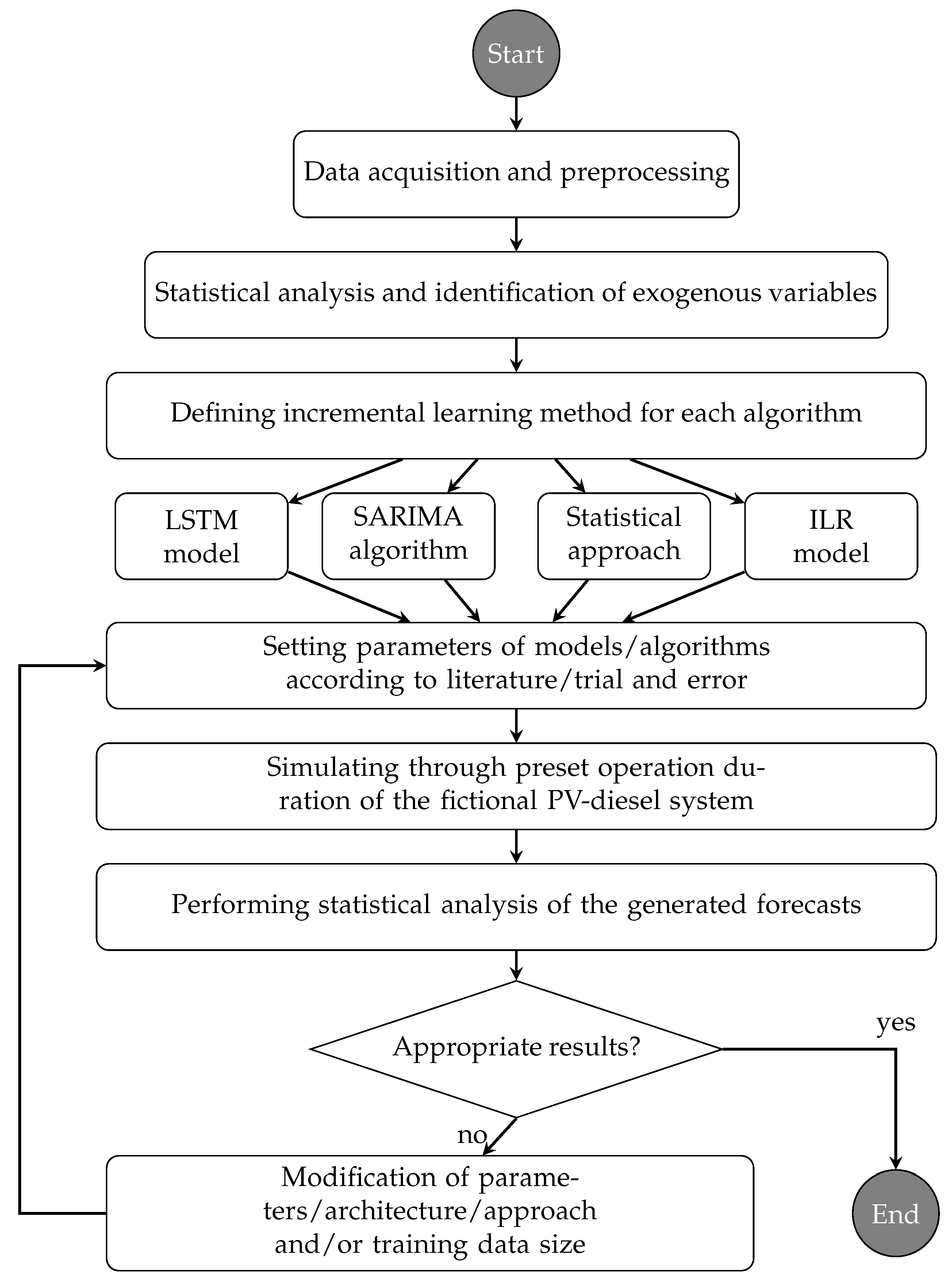
Funding

This research is part of the project EnerSHelF, which is funded by the German Federal Ministry of Education and Research as part of the CLIENT II program. Funding reference number: 03SF0567A-G.

Institutional Review Board Statement

The study was approved by the Ghana Health Service Ethics Review Committee (GHS-ERC) (GHS-ERC Number: GHS-ERC006/12/19 | date of approval: 30 January 2020).

Informed Consent Statement

Informed consent was obtained from all subjects involved in the study.

Data Availability Statement

Data not made publicly available due to ethical, legal and privacy limitations.

Acknowledgments

The authors would like to express their gratitude towards the project partners of the Father Franz Kruse Solar Energy Project in Akwatia in Ghana, i.e., the Diocese of Koforidua and the Bishop Most Reverend Joseph Afrifah-Agyekum, the management and staff of the St. Dominic’s Hospital in Akwatia, Kindermissionswerk, and Begeca as the funding organizations and Norbert Schneider for his initiative for the project. The authors would also like to thank our Ghanaian colleagues and partners for their support within the Client II project “EnerSHelF”.

Conflicts of Interest

The authors declare no conflict of interest. The funder had no role in the design of the study, in the collection, analyses, or interpretation of data, in the writing of the manuscript; or in the decision to publish the results.

Abbreviations

MPCModel predictive control
SARIMASeasonal autoregressive integrated moving average
LSTMLong short-term memory
nRMSENormalized root mean square error
PVPhotovoltaic
LCOELevelized cost of electricity
ILRIncremental linear regression
ARIMAAutoregressive integrated moving average
LOESSLocally estimated scatterplot smoothing
LEDLight-emitting diode
SDStandard deviation
PVGISPhotovoltaic geographical information system
ERA5European center for medium-range weather forecasts reanalysis 5th generation
CDDCooling degree day
ARMAAutoregressive moving average
RNNRecurrent neural network
BPTTBackpropagation through time
ADAMAdaptive moment estimation
MSEMean squared error
MAPEMean absolute percentage error
ReLURectified linear unit
EnerSHelFEnergy-self-sufficiency for health facilities in Ghana

References

  1. IEA. Africa Energy Outlook 2019; Technical Report; IEA: Paris, France, 2019. [Google Scholar]
  2. Adu, G.; Dramani, J.; Oteng-Abayie, E.F. Powering the Powerless: The Economic Impact of Rural Electrification in Ghana; Technical Report; The International Growth Centre (IGC): London, UK, 2018; Reference Number: E-33412-GHA-2. [Google Scholar] [CrossRef]
  3. Kumi, E. The Electricity Situation in Ghana: Challenges and Opportunities; Center for Global Development (CGD): Washington, DC, USA, 2017. [Google Scholar]
  4. Bertheau, P.; Oyewo, A.; Cader, C.; Blechinger, P. Visualizing National Electrification Scenarios for Sub-Saharan African Countries. Energies 2017, 10, 1899. [Google Scholar] [CrossRef] [Green Version]
  5. Blechinger, P.; Cader, C.; Oyewo, A.; Bertheau, P. Energy Access for Sub-Saharan Africa with the Focus on Hybrid Mini-Grids; Reiner Lemoine Institut (RLI): Berlin, Germany, 2016. [Google Scholar]
  6. Energy Commission of Ghana. Electricity Supply Plan for the Ghana Power System: An Outlook of the Power Supply Situation for 2020 and Highlights of Medium Term Power Requirements; Technical Report; Energy Commission of Ghana: Accra, Ghana, 2020. [Google Scholar]
  7. Apenteng, B.; Opoku, S.; Ansong, D.; Akowuah, E.; Afriyie-Gyawu, E. The effect of power outages on in-facility mortality in healthcare facilities: Evidence from Ghana. Glob. Public Health 2016, 13, 1–11. [Google Scholar] [CrossRef] [PubMed]
  8. Shihadeh, A.; Al Helou, M.; Saliba, N.; Jaber, S.; Alaeddine, N.; Ibrahim, E. Effect of distributed electric power generation on household exposure to airborne carcinogens in Beirut. Clim. Chang. Environ. Arab. World 2013. Available online: http://hdl.handle.net/10938/21130 (accessed on 12 January 2021).
  9. Sachs, J.; Sawodny, O. A Two-Stage Model Predictive Control Strategy for Economic Diesel-PV-Battery Island Microgrid Operation in Rural Areas. IEEE Trans. Sustain. Energy 2016, 7, 903–913. [Google Scholar] [CrossRef]
  10. Dongol, D. Development and Implementation of Model Predictive Control for a Photovoltaic Battery System. Ph.D. Thesis, Albert-Ludwigs-Universität Freiburg im Breisgau, Freiburg, Germany, 2019. [Google Scholar] [CrossRef]
  11. Chakhchoukh, Y.; Panciatici, P.; Mili, L. Electric Load Forecasting Based on Statistical Robust Methods. IEEE Trans. Power Syst. 2011, 26, 982–991. [Google Scholar] [CrossRef]
  12. Bozkurt, Ö.Ö.; Biricik, G.; Taysi, Z.C. Artificial neural network and SARIMA based models for power load forecasting in Turkish electricity market. PLoS ONE 2017, 12, e0175915. [Google Scholar] [CrossRef] [PubMed] [Green Version]
  13. Siami-Namini, S.; Namin, A.S. Forecasting Economics and Financial Time Series: ARIMA vs. LSTM. arXiv 2018, arXiv:1803.06386. [Google Scholar]
  14. Kong, W.; Dong, Z.Y.; Jia, Y.; Hill, D.J.; Xu, Y.; Zhang, Y. Short-Term Residential Load Forecasting Based on LSTM Recurrent Neural Network. IEEE Trans. Smart Grid 2019, 10, 841–851. [Google Scholar] [CrossRef]
  15. Bouktif, S.; Fiaz, A.; Ouni, A.; Serhani, M. Optimal Deep Learning LSTM Model for Electric Load Forecasting using Feature Selection and Genetic Algorithm: Comparison with Machine Learning Approaches. Energies 2018, 11, 1636. [Google Scholar] [CrossRef] [Green Version]
  16. Steinebach, G.; Jax, T.; Hausmann, P.; Dreistadt, D. ERWAS-Verbundprojekt EWave: Energiemanagementsystem Wasserversorgung-Abschlussbericht zu Teilprojekt 5; Hochschule Bonn-Rhein-Sieg: Sankt Augustin, Germany, 2018. [Google Scholar]
  17. Bruno, S.; Dellino, G.; La Scala, M.; Meloni, C. A Microforecasting Module for Energy Management in Residential and Tertiary Buildings. Energies 2019, 12, 1006. [Google Scholar] [CrossRef] [Green Version]
  18. Maitanova, N.; Telle, J.S.; Hanke, B.; Grottke, M.; Schmidt, T.; Maydell, K.V.; Agert, C. A Machine Learning Approach to Low-Cost Photovoltaic Power Prediction Based on Publicly Available Weather Reports. Energies 2020, 13, 735. [Google Scholar] [CrossRef] [Green Version]
  19. Diagne, H.; David, M.; Lauret, P.; Boland, J. Solar Irradiation Forecasting: State-of-the-Art and Proposition for Future Developments for Small-Scale Insular Grids; WREF 2012-World Renewable Energy Forum: Denver, CO, USA, May 2012. [Google Scholar]
  20. Yang, Y.; Che, J.; Li, Y.; Zhao, Y.; Zhu, S. An incremental electric load forecasting model based on support vector regression. Energy 2016, 113, 796–808. [Google Scholar] [CrossRef]
  21. De Silva, D.; Yu, X.; Alahakoon, D.; Holmes, G. Incremental pattern characterization learning and forecasting for electricity consumption using smart meters. In Proceedings of the 2011 IEEE International Symposium on Industrial Electronics, Gdansk, Poland, 27–30 June 2011; pp. 807–812. [Google Scholar] [CrossRef]
  22. Qiu, X.; Suganthan, P.N.; Amaratunga, G.A. Ensemble incremental learning Random Vector Functional Link network for short-term electric load forecasting. Knowl.-Based Syst. 2018, 145, 182–196. [Google Scholar] [CrossRef]
  23. Bouchachia, A.; Gabrys, B.; Sahel, Z. Overview of Some Incremental Learning Algorithms. In Proceedings of the 2007 IEEE International Fuzzy Systems Conference, London, UK, 23–26 July 2007; pp. 1–6. [Google Scholar] [CrossRef]
  24. Wang, H.; Chen, Q. Impact of climate change heating and cooling energy use in buildings in the United States. Energy Build. 2014, 82, 428–436. [Google Scholar] [CrossRef] [Green Version]
  25. Amato, A.; Ruth, M.; Kirshen, P.; Horwitz, J. Regional Energy Demand Responses to Climate Change: Methodology and Application to the Commonwealth of Massachusetts. Clim. Chang. 2005, 71, 175–201. [Google Scholar] [CrossRef]
  26. Ramírez-Sandí, S.; Quirós-Tortós, J. Evaluating the Effects of Climate Change on the Electricity Demand of Distribution Networks. In Proceedings of the 2018 IEEE PES Transmission Distribution Conference and Exhibition—Latin America (T D-LA), Lima, Peru, 18–21 September 2018; pp. 1–5. [Google Scholar] [CrossRef]
  27. Berger, M.; Worlitschek, J. The link between climate and thermal energy demand on national level: A case study on Switzerland. Energy Build. 2019, 202, 109372. [Google Scholar] [CrossRef]
  28. Jäger, J. Climate and Energy Systems: A Review of Their Interactions; International Series on Applied Systems Analysis; John Wiley & Sons: Chichester, UK, 1983; Volume 12. [Google Scholar]
  29. Simons, B.; Koranteng, C.; Adinyira, E.; Ayarkwa, J. An Assessment of Thermal Comfort in Multi Storey Office Buildings in Ghana. J. Build. Constr. Plan. Res. 2014, 2, 30–38. [Google Scholar] [CrossRef] [Green Version]
  30. Nwalusi, D.; Chukwuali, C.; Nwachukwu, M.; Chike, H. Analysis of Thermal Comfort in Traditional Residential Buildings in Nigeria. J. Recent Act. Arch. Sci. 2019, 4, 28–39. [Google Scholar] [CrossRef]
  31. Akande, O.; Adebamowo, M. Indoor Thermal Comfort for Residential Buildings in Hot-Dry Climate of Nigeria. In Proceedings of the Conference: Adapting to Change: New Thinking of Comfort, Cumberland Lodge, Windsor, UK, 9–11 April 2010. [Google Scholar]
  32. Van Rossum, G.; Drake, F.L., Jr. Python Reference Manual; Centrum voor Wiskunde en Informatica Amsterdam: Amsterdam, The Netherlands, 1995. [Google Scholar]
  33. Seabold, S.; Perktold, J. Statsmodels: Econometric and statistical modeling with python. In Proceedings of the 9th Python in Science Conference, Austin, TX, USA, 28 June–3 July 2010. [Google Scholar]
  34. Abadi, M.; Agarwal, A.; Barham, P.; Brevdo, E.; Chen, Z.; Citro, C.; Corrado, G.S.; Davis, A.; Dean, J.; Devin, M.; et al. TensorFlow: Large-Scale Machine Learning on Heterogeneous Systems. 2015. Available online: http://tensorflow.org (accessed on 12 January 2021).
  35. Sen, P.K. Estimates of the regression coefficient based on Kendall’s tau. J. Am. Stat. Assoc. 1968, 63, 1379–1389. [Google Scholar] [CrossRef]
  36. Mann, H.B. Nonparametric tests against trend. Econometrica 1945, 13, 245–259. [Google Scholar] [CrossRef]
  37. Kendall, M.G. Rank Correlation Methods; Griffin: London, UK, 1948. [Google Scholar]
  38. Huld, T.; Müller, R.; Gambardella, A. A new solar radiation database for estimating PV performance in Europe and Africa. Sol. Energy 2012, 86, 1803–1815. [Google Scholar] [CrossRef]
  39. Hersbach, H.; Bell, B.; Berrisford, P.; Hirahara, S.; Horányi, A.; Muñoz-Sabater, J.; Nicolas, J.; Peubey, C.; Radu, R.; Schepers, D.; et al. The ERA5 global reanalysis. Q. J. R. Meteorol. Soc. 2020. [Google Scholar] [CrossRef]
  40. Freedman, D.; Pisani, R.; Purves, R. Statistics (International Student Edition); W. W. Norton & Company: New York City, NY, USA, 2007. [Google Scholar]
  41. Benesty, J.; Chen, J.; Huang, Y.; Cohen, I. Pearson correlation coefficient. In Noise Reduction in Speech Processing; Springer: Berlin, Germany, 2009; pp. 1–4. [Google Scholar]
  42. Akoglu, H. User’s guide to correlation coefficients. Turk. J. Emerg. Med. 2018, 18. [Google Scholar] [CrossRef] [PubMed]
  43. Cohen, J. Statistical Power Analysis for the Behavioral Sciences; Academic Press: Cambridge, MA, USA, 2013. [Google Scholar]
  44. Sachs, J. Model-Based Optimization of Hybrid Energy Systems. Ph.D. Thesis, Universität Stuttgart, Stuttgart, Germany, 2016. [Google Scholar]
  45. Fang, T.; Lahdelma, R. Evaluation of a multiple linear regression model and SARIMA model in forecasting heat demand for district heating system. Appl. Energy 2016, 179, 544–552. [Google Scholar] [CrossRef]
  46. Vagropoulos, S.I.; Chouliaras, G.I.; Kardakos, E.G.; Simoglou, C.K.; Bakirtzis, A.G. Comparison of SARIMAX, SARIMA, modified SARIMA and ANN-based models for short-term PV generation forecasting. In Proceedings of the 2016 IEEE International Energy Conference (ENERGYCON), Leuven, Belgium, 4–8 April 2016; pp. 1–6. [Google Scholar] [CrossRef]
  47. Lee, C.M.; Ko, C.N. Short-term load forecasting using lifting scheme and ARIMA models. Expert Syst. Appl. 2011, 38, 5902–5911. [Google Scholar] [CrossRef]
  48. Goodfellow, I.; Courville, A.; Bengio, Y. Deep Learning: Das Umfassende Handbuch: Grundlagen, Aktuelle Verfahren und Algorithmen, Neue Forschungsansätze, 1st ed.; Verlags GmbH & Co. KG: Frechen, Germany, 2018. [Google Scholar]
  49. Hochreiter, S.; Schmidhuber, J. Long short-term memory. Neural Comput. 1997, 9, 1735–1780. [Google Scholar] [CrossRef]
  50. EnerSHelF-Energy-Self-Sufficiency for Health Facilities in Ghana. Available online: https://enershelf.de/ (accessed on 12 January 2021).
Figure 1. Flowchart of the research steps conducted in this study.
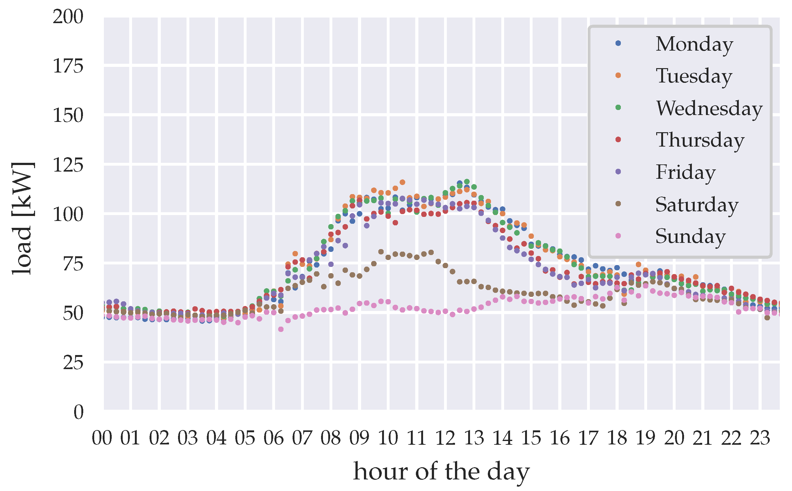
Energies 14 00409 g001
Figure 2. Mean load for the wet season 2015 (April–October), clustered by weekday.
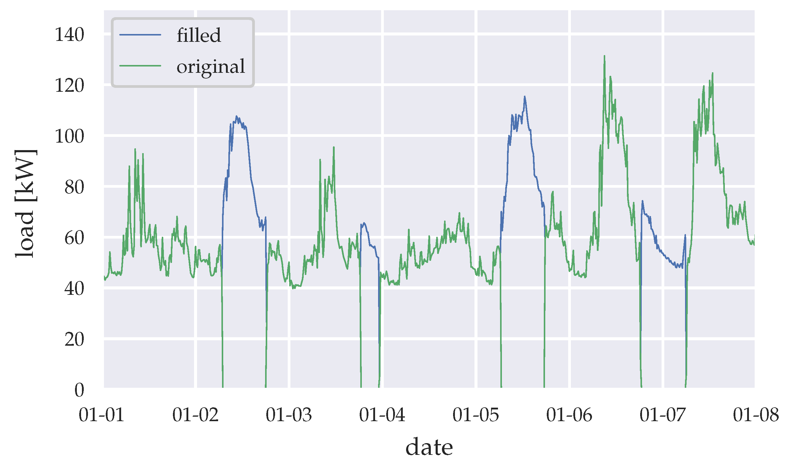
Energies 14 00409 g002
Figure 3. Data filling (example for the first week of 2015).
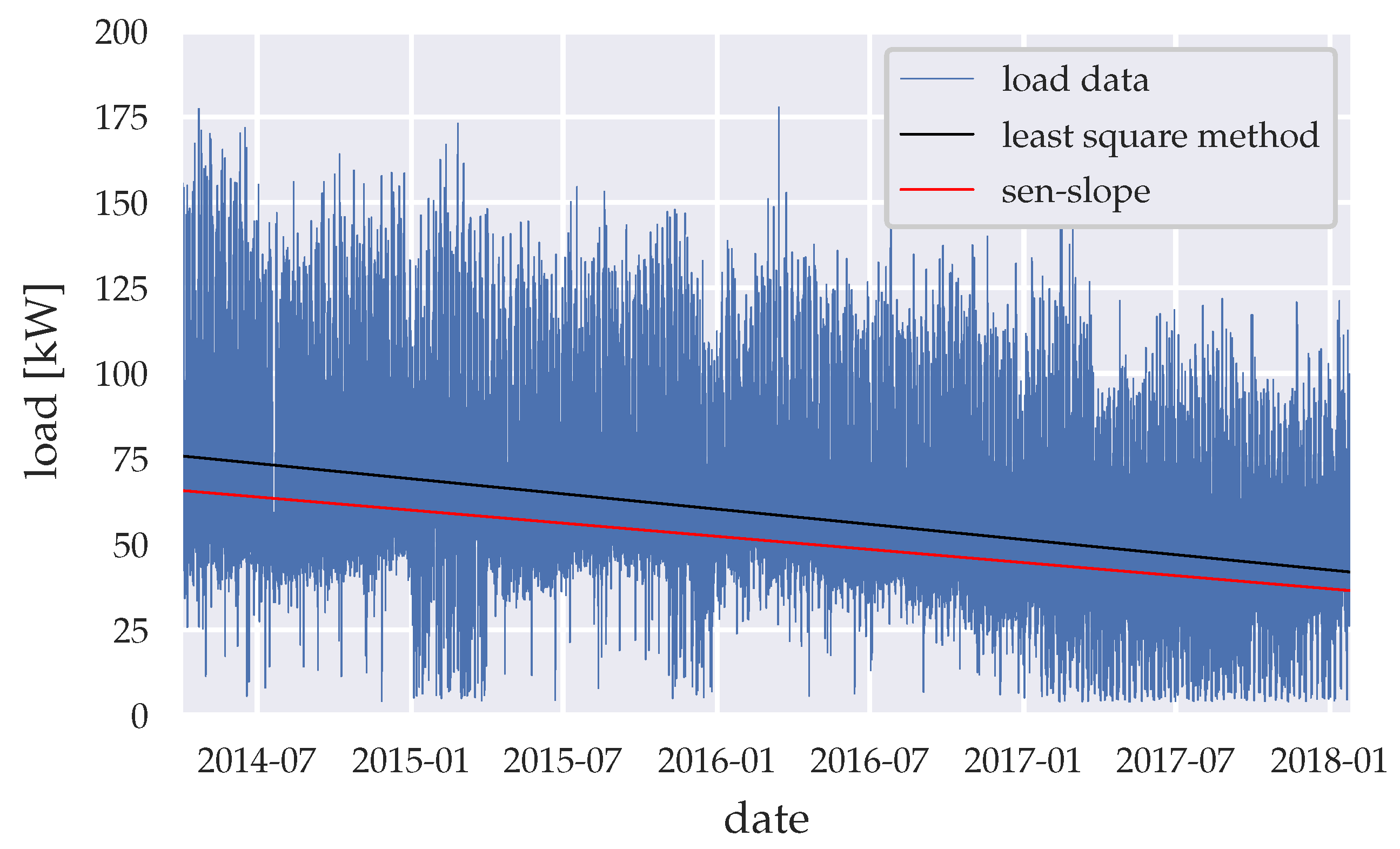
Energies 14 00409 g003
Figure 4. Load trend throughout the whole time-series period.
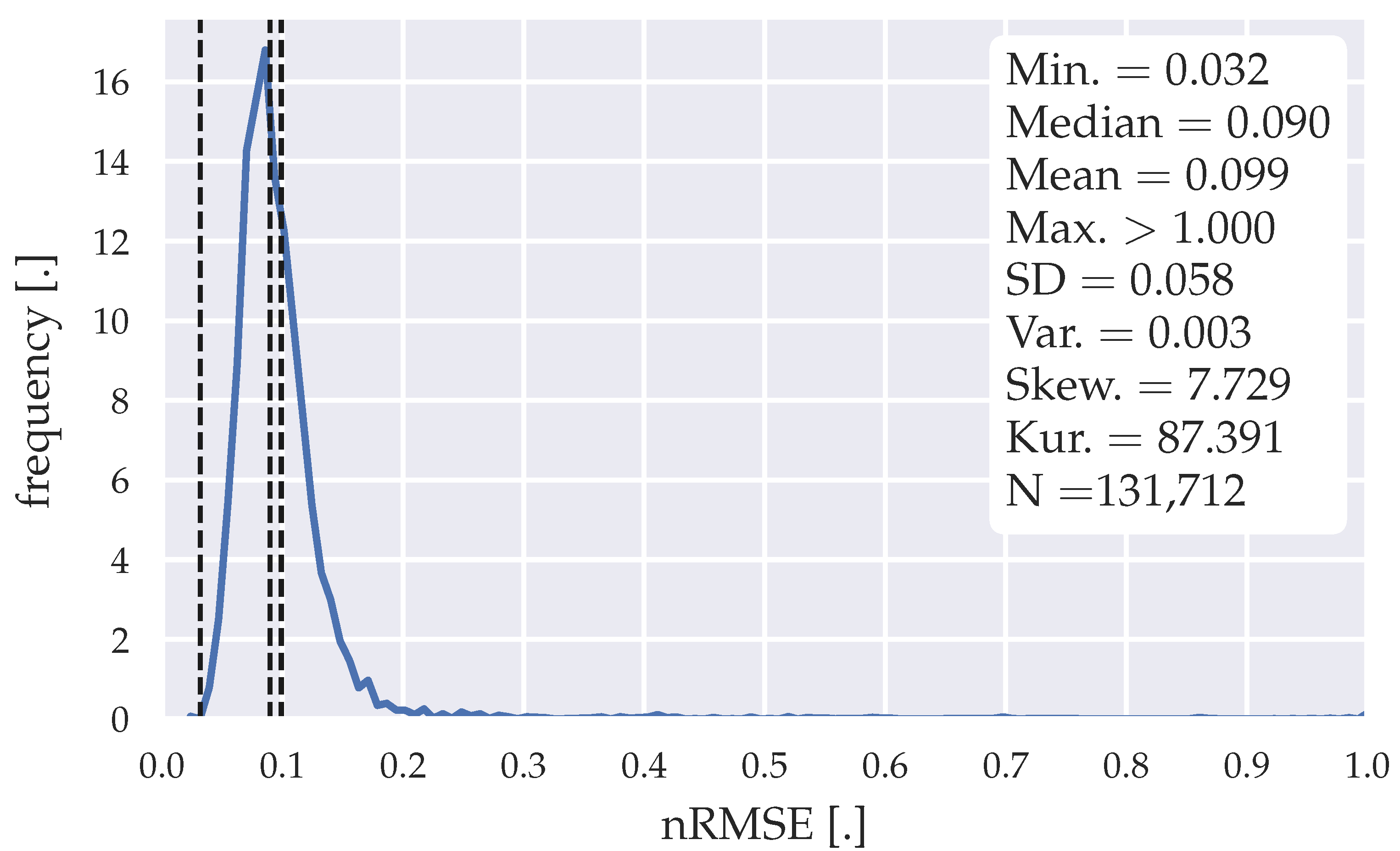
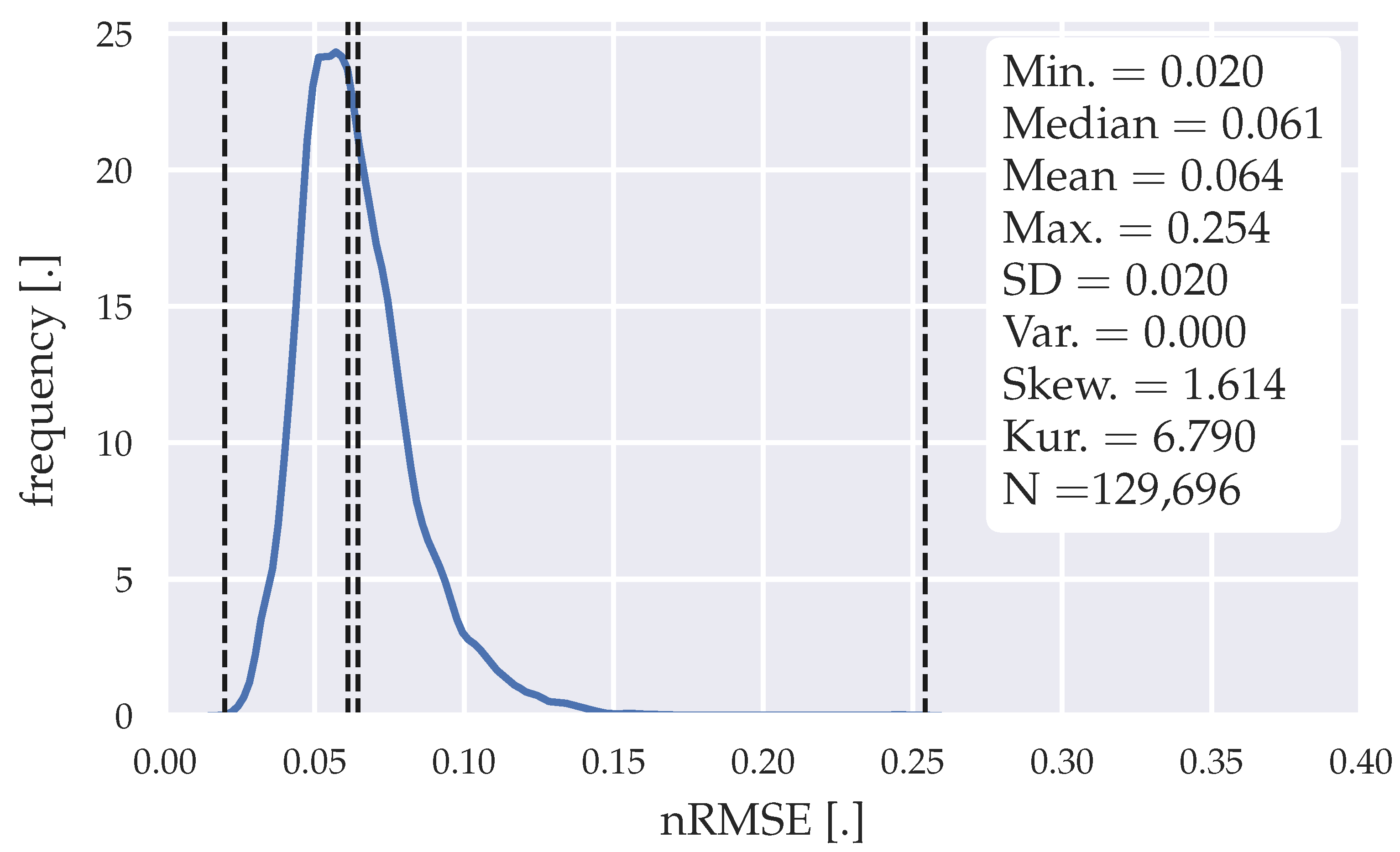
Energies 14 00409 g004
Figure 5. Error distribution of the forecasts generated with the statistical forecasting algorithm.
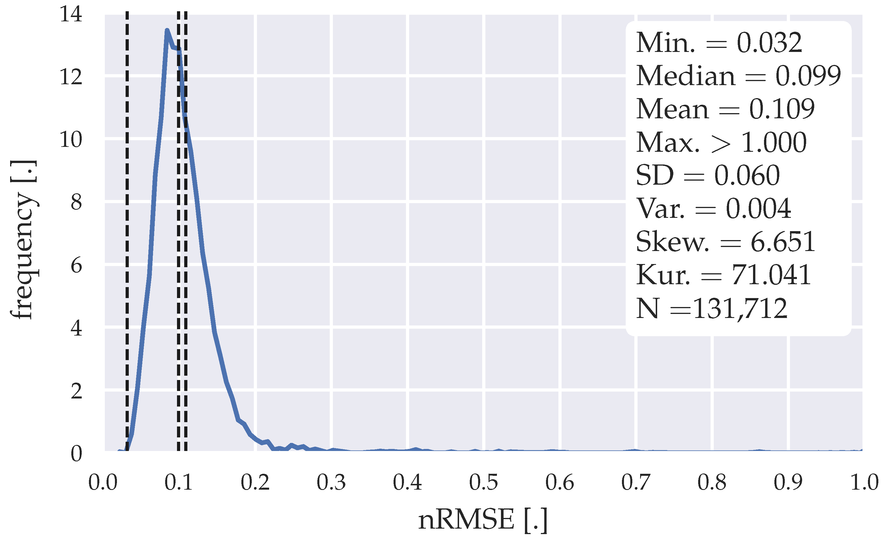
Energies 14 00409 g005
Figure 6. Error distribution of the forecasts generated with the SARIMA algorithm| SARIMA(1,1,1)(1,1,2)96 model.
Energies 14 00409 g006
Figure 7. Error distribution of the forecasts generated with the SARIMA algorithm| SARIMA(3,1,1)(0,1,2)96 model.
Energies 14 00409 g007
Figure 8. Error distribution of the forecasts generated with the LSTM model.
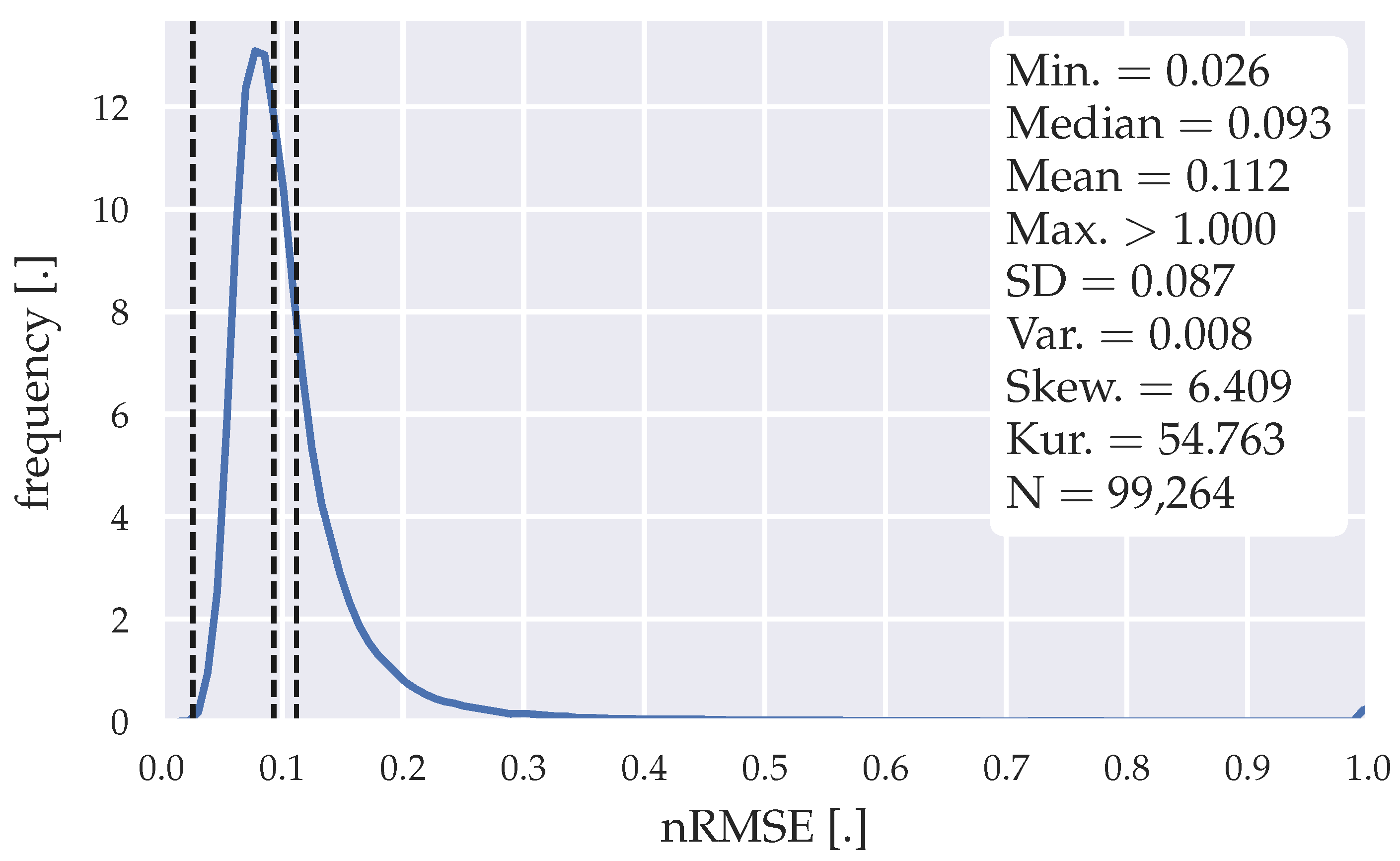
Energies 14 00409 g008
Figure 9. Error distribution of the forecasts generated with the ILR model.
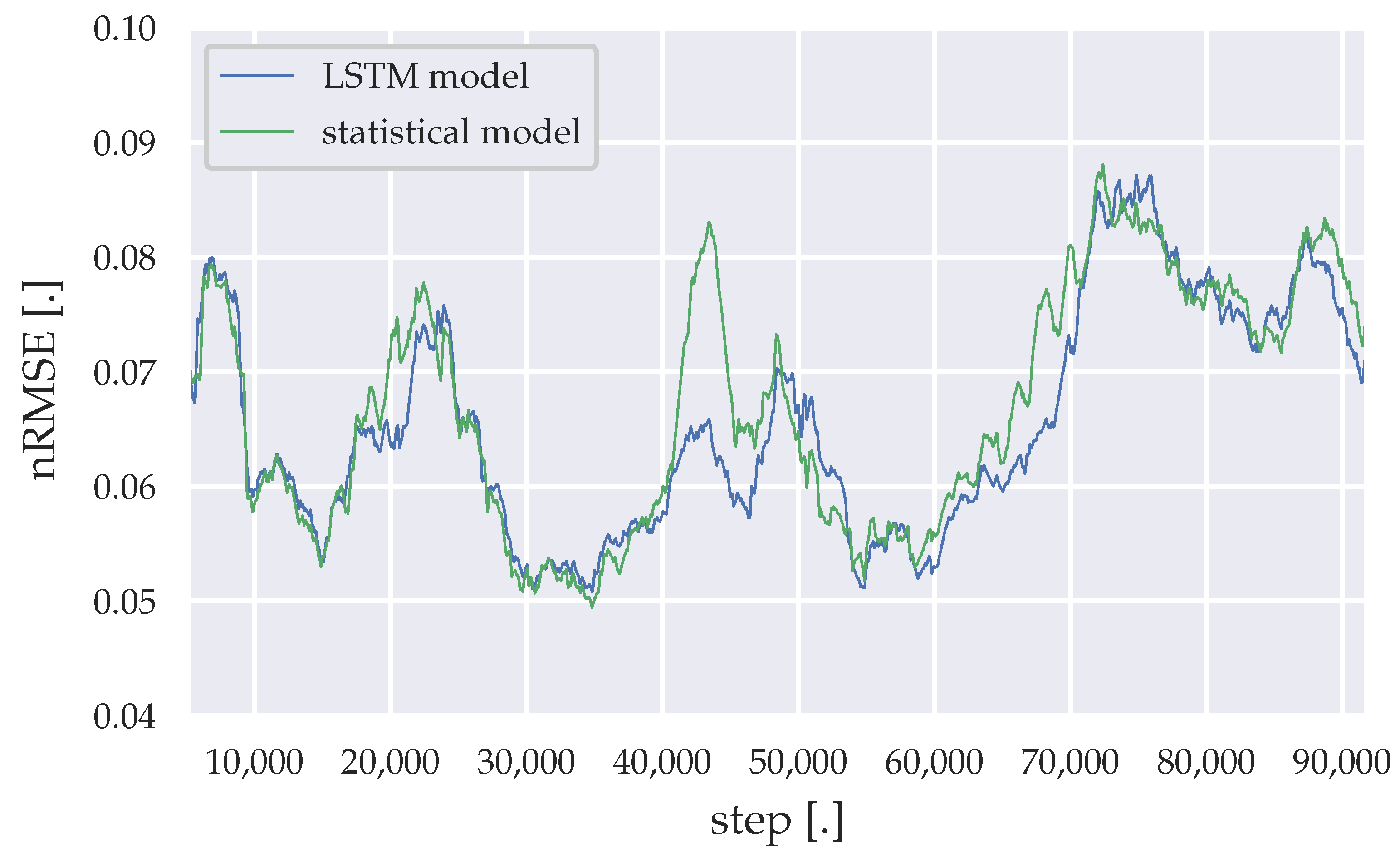
Energies 14 00409 g009
Figure 10. Moving average of the nRMSE generated by the LSTM model and the statistical algorithm (weekdays).
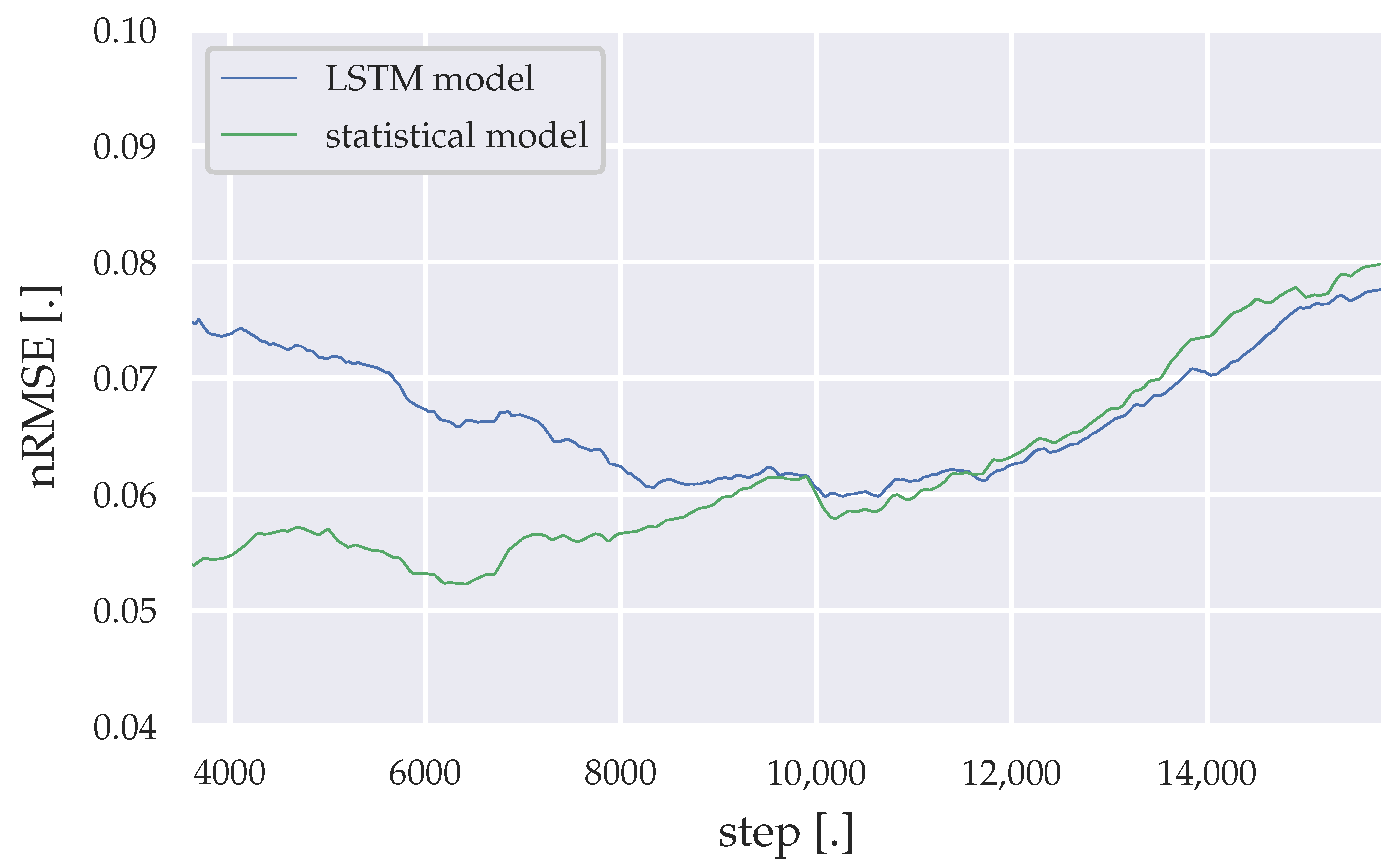
Energies 14 00409 g010
Figure 11. Moving average of the nRMSE generated by the LSTM model and the statistical algorithm (Saturdays).
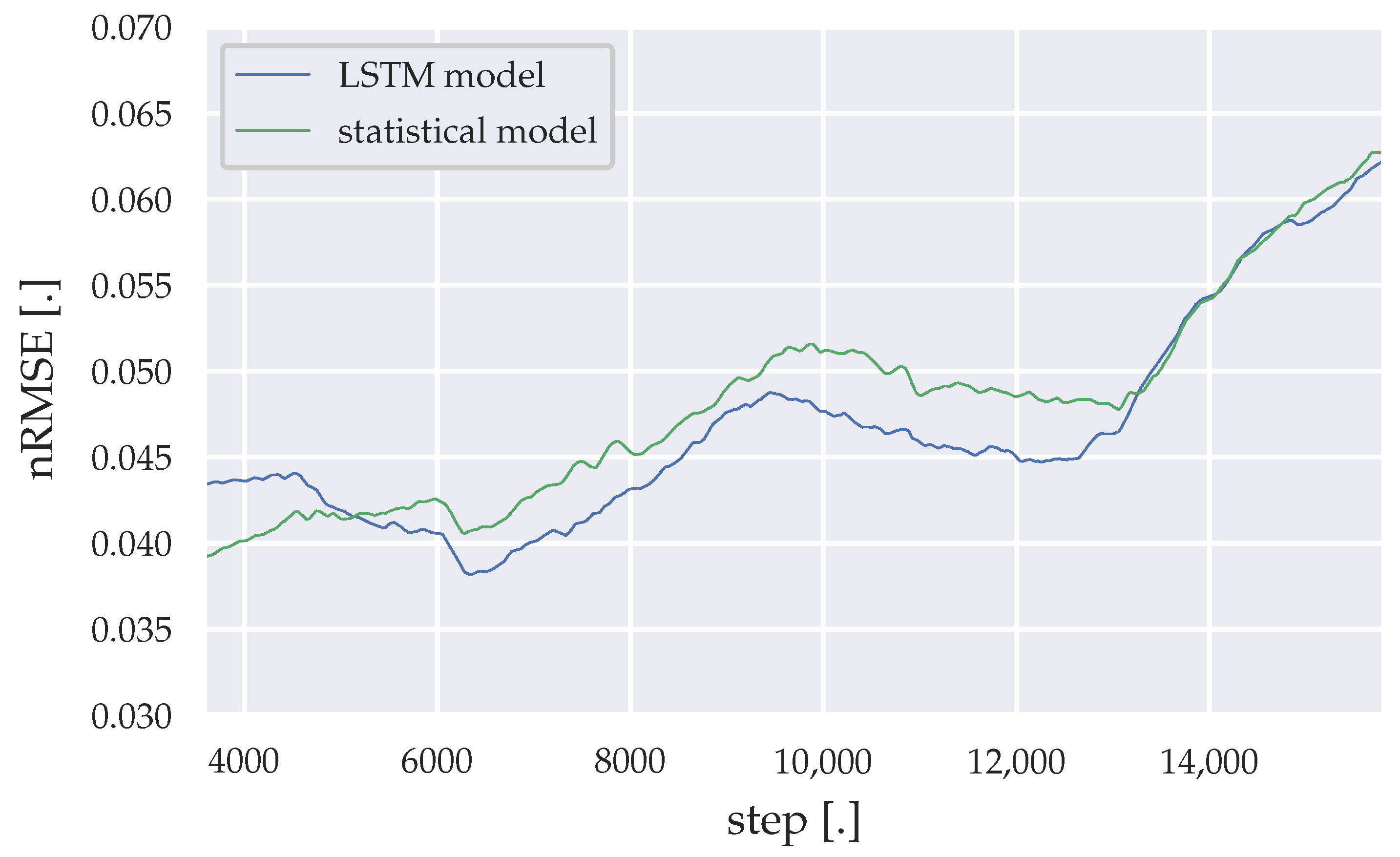
Energies 14 00409 g011
Figure 12. Moving average of the nRMSE generated by the LSTM model and the statistical algorithm (Sundays).
Energies 14 00409 g012
Table 1. Quantitative statistical evaluation, divided by years and seasons (wet: April–October|dry: November–March). “SD” stands for standard deviation. Values in kW, except variance.
YearPeriodMin.Max.MedianMeanQ0.05Q1Q3Q0.95SDVar.
2014Mar.–Dec.4.2177.3661.2869.5242.8851.0881.48121.9624.99624.51
wet season5.68177.3660.6868.9042.4050.3280.88121.7124.09629.60
dry season4.217563.0471.6245.5153.5283.17123.424.52601.33
2015Jan.–Dec.4.417359.7566.5742.4450.2577.77111.6322.10488.58
wet season4.44154.558.8665.7842.3850.0976.19109.521.29453.13
dry season4.417361.0667.6942.5950.4779.63115.0623.17536.70
2016Jan.–Dec.5.68177.7553.4958.8733.4143.7270.25100.8120.78431.75
wet season5.68155.553.459.0135.8443.7570.1999.8120.17406.87
dry season6.16177.7553.6958.6630.8443.5970.44101.8821.60466.74
2017Jan.–Dec.4.0154.8841.1944.3123.5633.1552.3877.6316.67278.00
wet season4.04121.8140.6943.3622.4832.4451.5375.0116.10259.23
dry season4.0154.8841.8845.6525.0834.0353.5681.1817.37301.55
2018Jan.–Feb.4.32121.1640.9243.4923.7833.7649.6975.7615.78249.04
Table 2. Mann–Kendall significance test, divided by years.
YearPeriodp-Valuez-Value
2014Mar.–Dec.0.0891.7
2015Jan.–Dec.<<0.05−14.13
2016Jan.–Dec.<<0.05−52.84
2017Jan.–Dec.<<0.05−17.26
2018Jan.–Feb.<<0.058.35
Table 3. Statistical results with different time frames, divided into the photovoltaic geographical information system (PVGIS) data set and the European center for medium-range weather forecasts 5th generation (ERA5) data set.
Data SetTimeframePearson’s r-Valuep-Value
PVGISwhole day0.54<<0.05
PVGISday-time0.2<<0.05
PVGISnight-time0.49<<0.05
ERA5whole day0.5<<0.05
ERA5day-time0.27<<0.05
ERA5night-time0.28<<0.05
Table 4. Statistical results of both data sets with the cooling degree day (CDD).
Data SetTimeframePearson’s r-Valuep-Value
PVGISwhole day−0.14<<0.05
ERA5whole day0.010.61
Table 5. Comparison of the normalized root-mean-square error (nRMSE), with different horizon configurations.
Horizon ConfigurationMin. nRMSEMed. nRMSEMean nRMSEMax. nRMSE
4 weeks0.0230.0650.0680.2
8 weeks0.0180.0650.0610.22
12 weeks0.0160.0650.0610.232
16 weeks0.0180.0650.0620.234
Table 6. Long short-term memory (LSTM) neural network architecture.
Layer-TypeAmount of CellsParametersActivation Function
LSTM9637,632rectified linear unit
LSTM192221,962rectified linear unit
fully connected neural network19237,056rectified linear unit
fully connected neural network9618,528rectified linear unit
Table 7. Fitting settings for each neural network.
TypeEpochsBatch SizeLoss FunctionOptimizer
initial weekday512mean squared erroradaptive moment estimation
initial saturday512mean squared erroradaptive moment estimation
initial sunday56mean squared erroradaptive moment estimation
continous weekday212mean squared erroradaptive moment estimation
continous saturday212mean squared erroradaptive moment estimation
continous sunday26mean squared erroradaptive moment estimation
Table 8. nRMSE with different prediction horizons|statistical forecasting algorithm.
Prediction HorizonMin. nRMSEMedian nRMSEMean nRMSEMax. nRMSE
3 h0.0030.0470.0560.41
6 h0.0040.0510.0580.385
9 h0.0050.0540.0600.338
12 h0.0090.0560.0620.302
15 h0.0110.0580.0630.272
18 h0.0150.0600.0640.25
21 h0.0180.0610.0640.234
24 h0.0180.0610.0650.220
Table 9. Computational effort for the statistical forecasting method, divided in weekday, Saturday, and Sunday batching, clustered in training and prediction efforts.
TypeData BatchingMedian Computation TimeOverall Computation Time
trainingweekday0.067 ms131.428 ms
Saturday0.064 ms12.229 ms
Sunday0.014 ms2.763 ms
predictionweekday0.032 ms2.905 s
Saturday0.029 ms0.446 s
Sunday0.029 ms0.452 s
Table 10. nRMSE with different prediction horizons|SARIMA(1,1,1)(1,1,2)96 model.
Prediction HorizonMin. nRMSEMedian nRMSEMean nRMSEMax. nRMSE
3 h00.0700.086>1
6 h00.0750.09>1
9 h0.0020.0810.094>1
12 h0.0050.0870.098>1
15 h0.0210.0910.102>1
18 h0.0280.0950.105>1
21 h0.0290.0970.107>1
24 h0.0320.0990.109>1
Table 11. nRMSE with different prediction horizons|SARIMA(3,1,1)(0,1,2)96 model.
Prediction HorizonMin. nRMSEMedian nRMSEMean nRMSEMax. nRMSE
3 h00.0660.081>1
6 h0.0020.0710.085>1
9 h0.0020.0760.088>1
12 h0.0030.0800.091>1
15 h0.0180.0840.094>1
18 h0.0260.0860.096>1
21 h0.0290.0880.098>1
24 h0.0320.090.099>1
Table 12. Computational effort for both SARIMA configurations, divided in weekday, Saturday, and Sunday batching, clustered in training and prediction efforts.
ConfigurationTypeData BatchingMedian Computation TimeOverall Computation Time
SARIMA 1,1,1, 1,1,2trainingweekday17.580 s4.787 h
Saturday22.403 s1.221 h
Sunday17.075 s0.931 h
predictionweekday0.488 ms46.440 s
Saturday0.510 ms8.546 s
Sunday0.490 ms10.505 s
SARIMA 3,1,1, 0,1,2trainingweekday20.141 s5.484 h
Saturday22.323 s1.216 h
Sunday17.041 s0.928 h
predictionweekday0.460 ms45.660 s
Saturday0.499 ms8.678 s
Sunday0.481 ms8.348 s
Table 13. nRMSE with different prediction horizons|LSTM model.
Prediction HorizonMin. nRMSEMedian nRMSEMean nRMSEMax. nRMSE
3 h0.0020.0480.0580.376
6 h0.0060.0530.060.287
9 h0.0070.0560.0620.26
12 h0.0110.0580.0630.279
15 h0.0180.0590.0640.281
18 h0.0190.060.0640.276
21 h0.020.0610.0640.266
24 h0.020.0610.0640.254
Table 14. Computational effort for the LSTM model, divided in weekday, Saturday, and Sunday batching, clustered in training and prediction efforts.
TypeData BatchingMedian Computation TimeOverall Computation Time
trainingweekday6.941 s22.115 min
Saturday4.783 s26.326 min
Sunday4.784 s26.272 min
predictionweekday39.987 ms61.786 min
Saturday40.106 ms25.761 min
Sunday40.108 ms25.696 min
Table 15. nRMSE with different prediction horizons|ILR method.
Prediction HorizonMin. nRMSEMedian nRMSEMean nRMSEMax. nRMSE
3 h0.0030.0630.086>1
6 h0.0070.0750.096>1
9 h0.0120.0820.102>1
12 h0.0170.0870.105>1
15 h0.0180.0900.108>1
18 h0.0210.0920.11>1
21 h0.0250.0930.111>1
24 h0.0260.0930.112>1
Table 16. Computational effort for the ILR method, clustered in initial training, training, and prediction efforts.
TypeMedian Computation TimeOverall Computation Time
initial training-0.125 ms
training0.126 ms12.630 s
prediction21.406 ms31.584 min
Table 17. nRMSE comparison of all algorithms, with a forecasting horizon of 24 h.
AlgorithmMin. nRMSEMedian nRMSEMean nRMSEMax. nRMSE
LSTM model0.020.0610.0640.376
statistical algorithm0.0180.0610.0650.22
SARIMA 1,1,1 1,1,20.0320.0990.109>1
SARIMA 3,1,1 0,1,20.0320.090.099>1
ILR algorithm0.0180.0900.108>1
Table 18. Descriptive statistics of the moving average nRMSE, generated by the LSTM model and the statistical algorithm (weekdays).
ModelMin.Max.MeanMedian
LSTM model0.0510.0870.0650.063
statistical algorithm0.0490.0880.0670.066
Table 19. Descriptive statistics of the moving average nRMSE, generated by the LSTM model and the statistical algorithm (Saturdays).
ModelMin.Max.MeanMedian
LSTM model0.0600.0780.0670.066
statistical algorithm0.0520.0790.0610.059
Table 20. Descriptive statistics of the moving average nRMSE, generated by the LSTM model and the statistical algorithm (Sundays).
ModelMin.Max.MeanMedian
LSTM model0.0380.0620.0470.046
statistical algorithm0.0390.0610.0480.048
Publisher’s Note: MDPI stays neutral with regard to jurisdictional claims in published maps and institutional affiliations.

