Construction of a Frequency Compliant Unit Commitment Framework Using an Ensemble Learning Technique

Abstract

Frequency control is essential to ensure reliability and quality of power systems. North American Electric Reliability Corporation’s (NERC) Control Performance Standard 1 (CPS1) is widely adopted by many operating authorities to examine the quality of the frequency control. The operating authority would have a strong interest in knowing how the frequency-sensitive features affect the CPS1 score and finding out more effective unit-dispatch schedules for reaching the CPS1 goal. As frequency-sensitive features usually possess multi-variable and high-correlated characteristics, this paper employed an ensemble learning technique (the Gradient Boosting Decision Tree algorithm, GBDT) to construct Frequency Response Model (FRM) of the Taipower system in Taiwan to evaluate by CPS1 score. The proposed CPS1 model was then integrated with Unit Commitment (UC) program to determine the unit-dispatch that achieves the targeted CPS1 score. The feasibility and effectiveness of the proposed CPS1-UC platform were validated and compared with the other benchmark model-based UC methods by two operating cases. The proposed model shows promising results: the system frequency could be maintained well, especially in the periods of the early morning or the high renewable penetration.

1. Introduction

The problem of determining the optimal unit commitment (UC) in power generation systems is solved by minimizing the total system cost while maintaining the load generation balance. At early stages, traditional UC are mainly based on cost considerations with unit and transmission security constraints. However, with the growing global emphasis on reduced emissions and renewable penetration, the UC model has recently been modified to take better account of the need for emission reduction or increased renewable resources during the power generation process [1,2,3,4,5].

Nevertheless, ensuring satisfactory frequency quality is still one of the most important practical concerns. The metric for evaluating frequency quality is usually referred to as the North American Electric Reliability Corporation’s (NERC) two Control Performance Standards (CPS1 and CPS2) [6]. The CPS score (i.e., frequency response quality index) could be affected by the generator type, load characteristics, regulation reserve, and the nature of the system itself (i.e., interconnection or island). Thus, each Independent System Operator (ISO) in North America has formulated its own requirements for the regulation reserve based on its own particular system [7].

In recent years, several statistical-based methods have been proposed to evaluate the CPS score by constructing a reference based on the load frequency control (LFC) model or UC model. For example, Chung developed an artificial neural network (ANN) algorithm to improve the CPS score by estimating the area control error (ACE) of the LFC model [8]. Some studies built up frequency constraints on specific generating units within the UC model [9,10,11,12]. Zhang established a low-order LFC model to calculate the CPS score training set (including CPS1 and the balancing authority ACE limit (BAAL)), then used a multiple linear regression (MLR) to determine the regulation reserve required to satisfy the target CPS1 score [13]. Yang used a cumulative distribution function (CDF) method to analyze the relationships between the automatic generation control (AGC) ramp rate, the droop response capability, and the CPS1 score [14].

The constructed models in the aforementioned studies are of reduced-order or linear fashions. However, the influential frequency-sensitive features are not only complicated by the nonlinearities of the real-world power system but correlated with each other. Consequently, the results obtained from some specific hours could differ a lot as the system frequency responses are evaluated by the reduced-order models. Conversely, in order to estimate the frequency responses of the real-world power system, more intelligent approaches are needed to cope with the multivariate and nonlinear problems. Nowadays, the supervised machine learning algorithms such as support vector machine (SVM), decision tree, deep learning and gradient boost decision tree (GBDT) [15,16,17,18,19], are able to identify the multivariate and nonlinearities of the system. Therefore, this paper attempts to introduce the supervised machine learning algorithm to construct the frequency response model (FRM), and integrate the model into the unit commitment program. The main contributions of this research are summarized as follows:

(1)

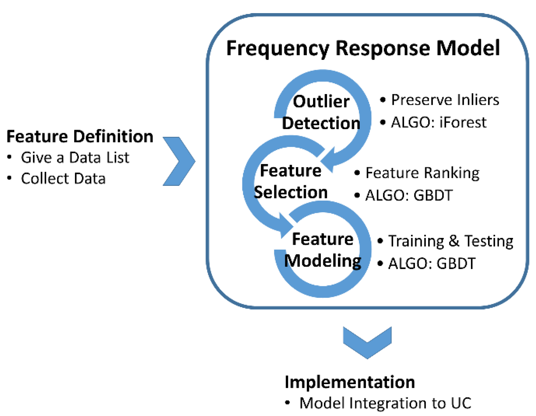
This study commences by employing an ensemble machine learning technique to formulate a robust FRM. For the formulation process, the ensemble learning technique can not only deal with data refinement, such as outlier detection and feature selection, but also feature modeling based on the operation’s domain knowledge.

(2)

The FRM model that is formulated by the ensemble learning technique is able to conform to the frequency response of the actual system from time to time by automatically tuning the hyperparameters within the model.

(3)

The well-trained FRM model is further integrated with a UC program to determine the unit scheduling result. Testing results show that the proposed solution not only ensures the compliance of the unit dispatch schedule to the NERC’s CPS1 standard, but also further minimizes the system operating cost compared to that of the real dispatch history.

(4)

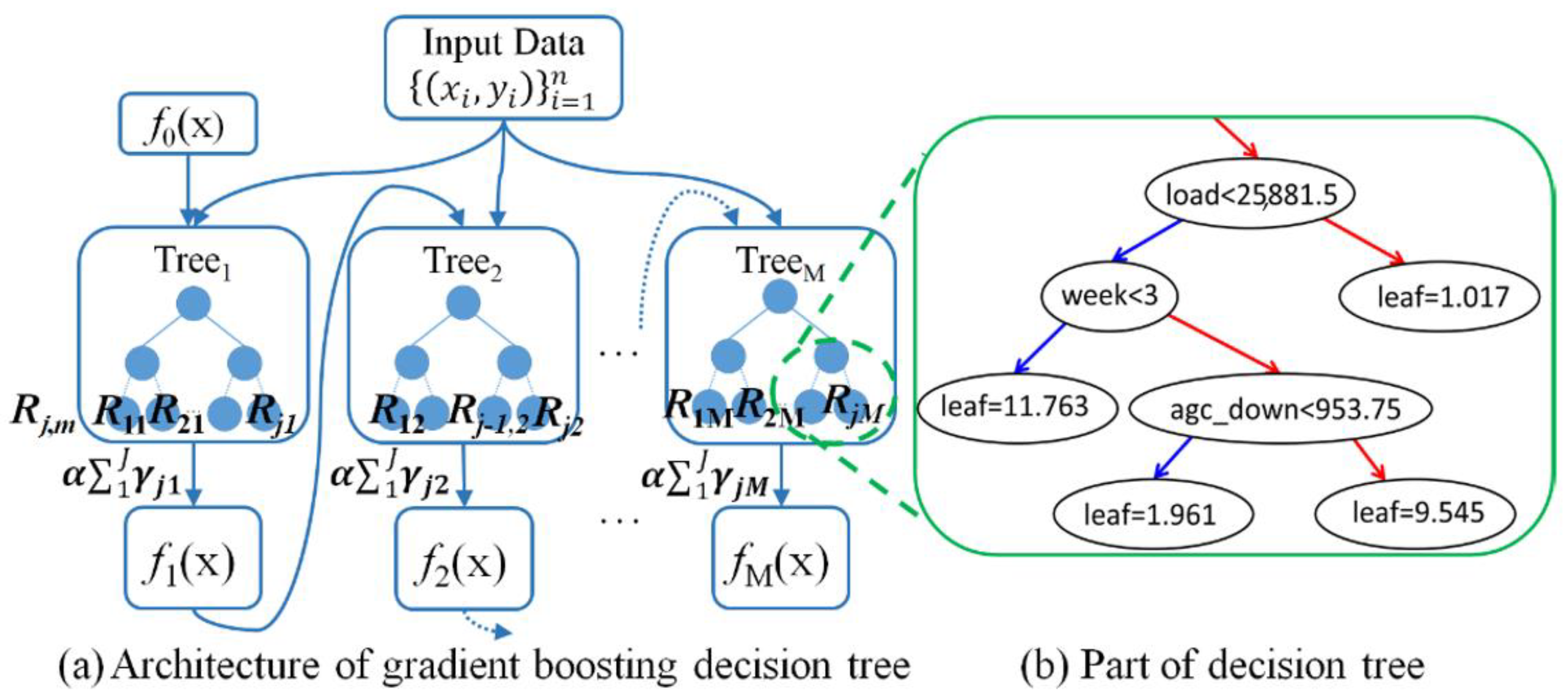
Comparative results from different methodologies have shown that the proposed FRM model is superior in portraying system frequency response over the simplified model that did not take the multivariate and nonlinear characteristics into account. Moreover, the proposed tree-based learning technique has shown its advantage in portraying the system state with more accurate feature interpretation over the neural-network based technique.

(5)

The proposed hybrid model (FRM plus UC) can portray different hypothetical cases, such as renewable penetration into the power system, for system operators to foresee the challenges they could face.

The remainder of this paper is organized as follows. Section 2 describes the data analysis process applied to the historical data and introduces the ensemble learning approach employed to construct a FRM (i.e., CPS1-compliant model) based on the frequency-sensitive features. Section 3 presents the frequency-constrained UC program for CPS1-compliant scheduling. Section 4 describes the integration of the FRM to perform CPS-compliant unit scheduling. Section 5 demonstrates the validity and effectiveness of the proposed scheduling method through two case studies. Finally, Section 6 presents concluding remarks and suggests avenues for future research.

2. Construction of the CPS1 Compliant Model

The conventional wisdom to model a complicated system generally involves in identifying key features that have influential impacts on the system behavior, followed by the model construction by interlinking the features with model parameters. To make the features effectively exert the model to closely trace the real system behavior, hyperparameter tuning is essential. This work is done either by going through a regression method or an intelligent training. Once the model validation is confirmed, the finely turned model could be gainfully used for the other applications, such as unit commitment program in this study.

Generally speaking, feature identification as well as the model parameter tuning are considered as the most complicated parts in system modeling because they usually involve in multivariate and highly correlated functions which cannot be easily grasped by the traditional linear system approach. Until the recent development of machine learning techniques, the accuracy of the complex system model could be elevated to a higher level. Figure 1 demonstrates the example of system modeling procedure using the machine learning algorithms. The construction of the CPS1-compliance model using the same procedure will be detailed in the following subsections.

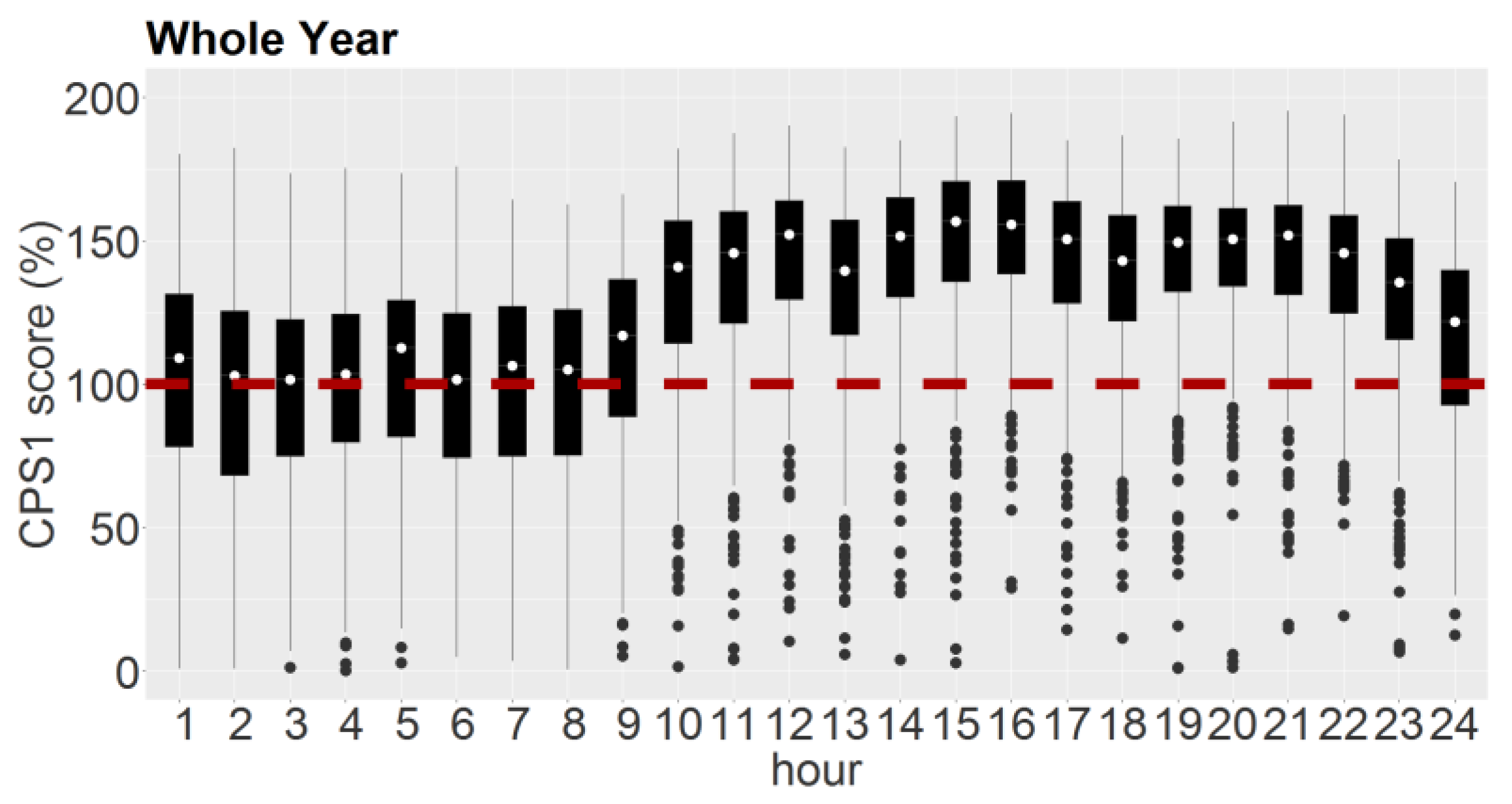
2.1. Exploratory Data Analysis for CPS1 in Taipower System (Feature Definition)

The Taipower system is an independent power system, with no interconnected ties to the neighboring areas. Since the load-generation balance is solely reflected by the system frequency, Taipower company abides by the CPS1 compliance rule (i.e., the system frequency quality index), which is the same as the metric adopted by the Electric Reliability Council of Texas (ERCOT) system in Texas (USA). Since the Taipower system is an isolated power system, therefore, the CPS1 score was calculated by Equation (1), which is shown as follows [6]:

$$CPS1=\left(2-\frac{AV{G}_T{\left(F_n-F_t\right)}^2}{{\epsilon }^2}\right)\times 100\%,$$

(1)

where AVG_T represents the averaging window within T periods; F_n is the actual frequency; F_t is the target frequency; ε is the target noise and is equal to 30 mHz in TPC’s case.

To better identify which the system states significantly influence the CPS1 record, an exploratory data analysis (EDA) method was employed to analyze the hourly operational data of the Taipower system. Figure 2 shows the average hourly CPS1 scores over the 12-month period. Note that for each hour, the white spot indicates the average CPS1 score, the black bars indicate the range of CPS1 scores, and the red dashed line represents the threshold of the CPS1 score (i.e., 100%). In general, the results show that the CPS1 scores of the first-shift period (i.e., 00:00 to 08:00) were lower than those of the other periods, with more than half of the scores failing to meet the target requirement of 100%.

Given the results presented in Figure 2, the present study aims to improve the frequency quality of the Taipower system to increase the CPS1 score in the first-shift period. Following lengthy discussions with the Taipower dispatchers, 11 frequency-sensitive features were identified as shown in

Table 1. Frequency-sensitive features for the Taipower system.

Feature	Label	Definition	Unit
Input
x1	Hour	Hour of day	Hour
x2	Week	Week	Week
x3	Month	Month	Month
x4	Load	Load demand during each hour	MWh
x5	Load Var	Load variance between two adjacent hours	MWh
x6	Ramp Rate	Capability of changing output in minute	MW/min
x7	AGC Up	Margin of up-regulation (secondary control)	MW
x8	AGC Down	Margin of down-regulation (secondary control)	MW
x9	Inertia	Inertia of power plant unit	second
x10	Pumping Load	Pumping load demand of Pumped-Storage Hydro Units (PSHUs)	MWh
x11	Pumping Load Var	Pumping load variance of Pumped-Storage Hydro Units (PSHUs)	MWh
Output
y1	CPS1	CPS1 score (Equation (1))	%

. Features x1 to x3 are time-dependent, while features x6 to x11 relate to the generating unit. Among these latter features, x6 to x8 relate to the AGC signal control. Feature x9 relates to the inertia of the parallel units, where a larger inertia value results in a more stable system frequency. Features x10 and x11 refer to the pumped-storage hydro units (PSHUs) pumping load operation. According to Taipower’s operation rule, PSHUs are operated mainly in the pumping mode during the first-shift period. Finally, feature y1 refers to the CPS1 score and is obtained by averaging the hourly values.

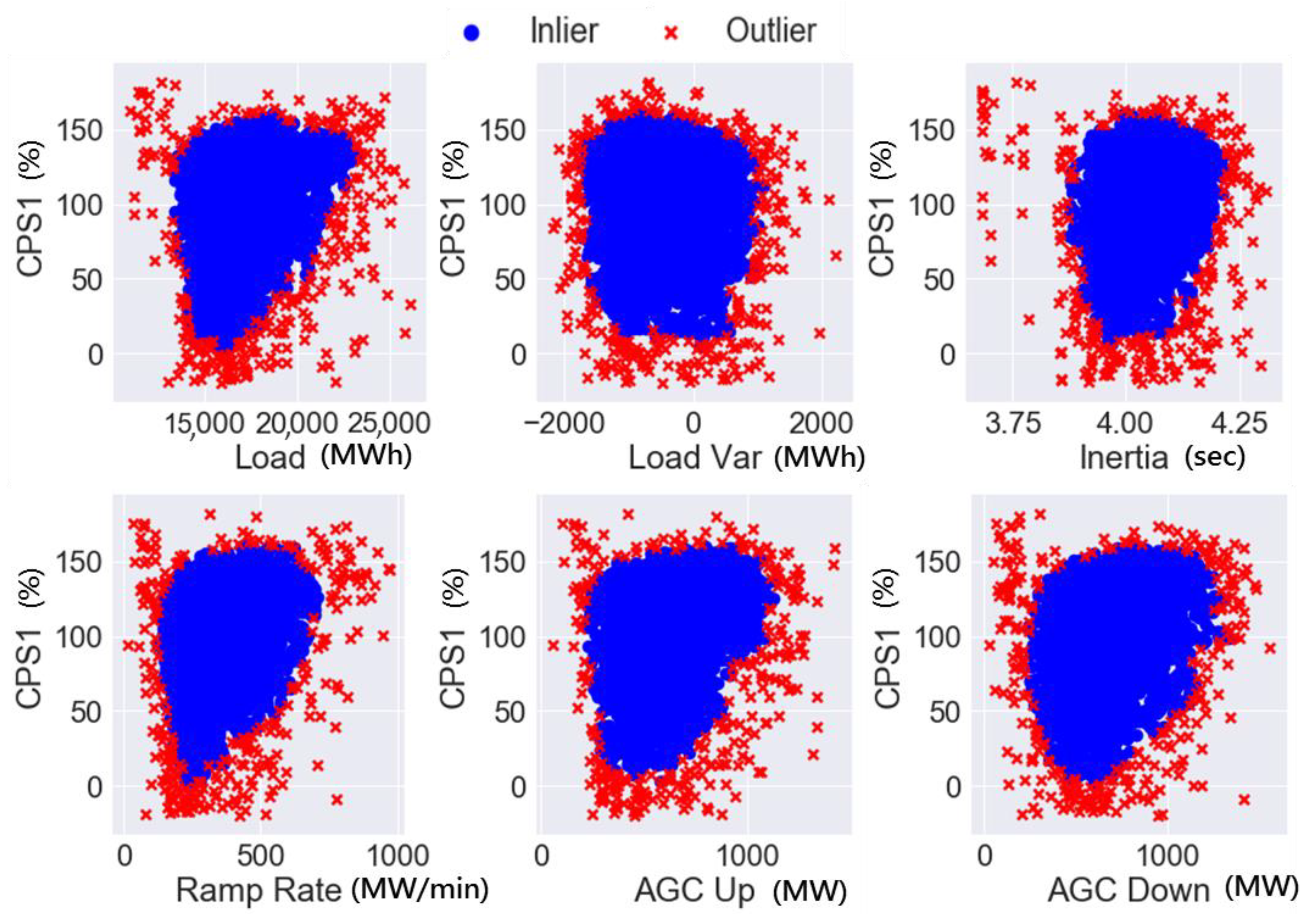
2.2. Outlier Detection

As the outliers are unlabeled in the present study, an unsupervised ensemble learning algorithm is required to perform outlier detection. Reference [20] evaluates the average accuracy, stability, computing time, and memory usage degree of 14 common unsupervised algorithms when applied to large-scale public and industrial datasets. The results showed that the isolation forest (iForest) algorithm performed better in identifying outliers than probabilistic methods such as probabilistic principal component analysis (PPCA), neural network methods such as grow when required (GWR), domain-based methods such as a one-class SVM, and distance-based methods such as the Mahalanobis distance. iForest is an ensemble method composed of multiple binary iTrees. The iForest algorithm has the following four main advantages for large-scale optimization-type problems: (1) it does not need to calculate the distance and density of the samples, and hence, the computational load and computing time are reduced; (2) the computing time scales proportionally with the size of the dataset); (3) the accuracy improves as the data volume increases; and (4) only a few hyperparameters must be set in advance [21].

Having constructed the iForest, the path length of sample p is normalized by the average path length of the whole sample, and the outlier score of sample p is calculated according to Equation (2). The samples are then sorted in accordance with their outlier scores [21]:

$$s\left(p,n\right)=2^{-\frac{E\left(h\left(p\right)\right)}{c\left(n\right)}},$$

(2)

where s(p, n) is the outlier score; h(p) is the path length of sample x in the iTree; E(h(p)) is the mean height of multiple iTrees h(p); and c(n) is the average path length of the iTree constructed by n samples.

In our case, the 11 frequency-sensitive features, which are identified in Table 1, were separately applied to the iForest algorithm for outlier detection. In the implementation of the iForest algorithm, the hyperparameters were specified as follows: (1) a subsample size of 256, (2) a tree depth of 8, and a forest size of 100 (trees). In other words, for each feature, 256 independent samples were randomly selected to constitute an iTree with a maximum depth of 8; at most, 100 iTrees were constructed.

Figure 3 shows the outlier detection results for six of the frequency-sensitive features. The results confirm that the detected outliers are all located at the periphery. The inliers were then used for further feature selection and modeling purposes, which will be described in next section.

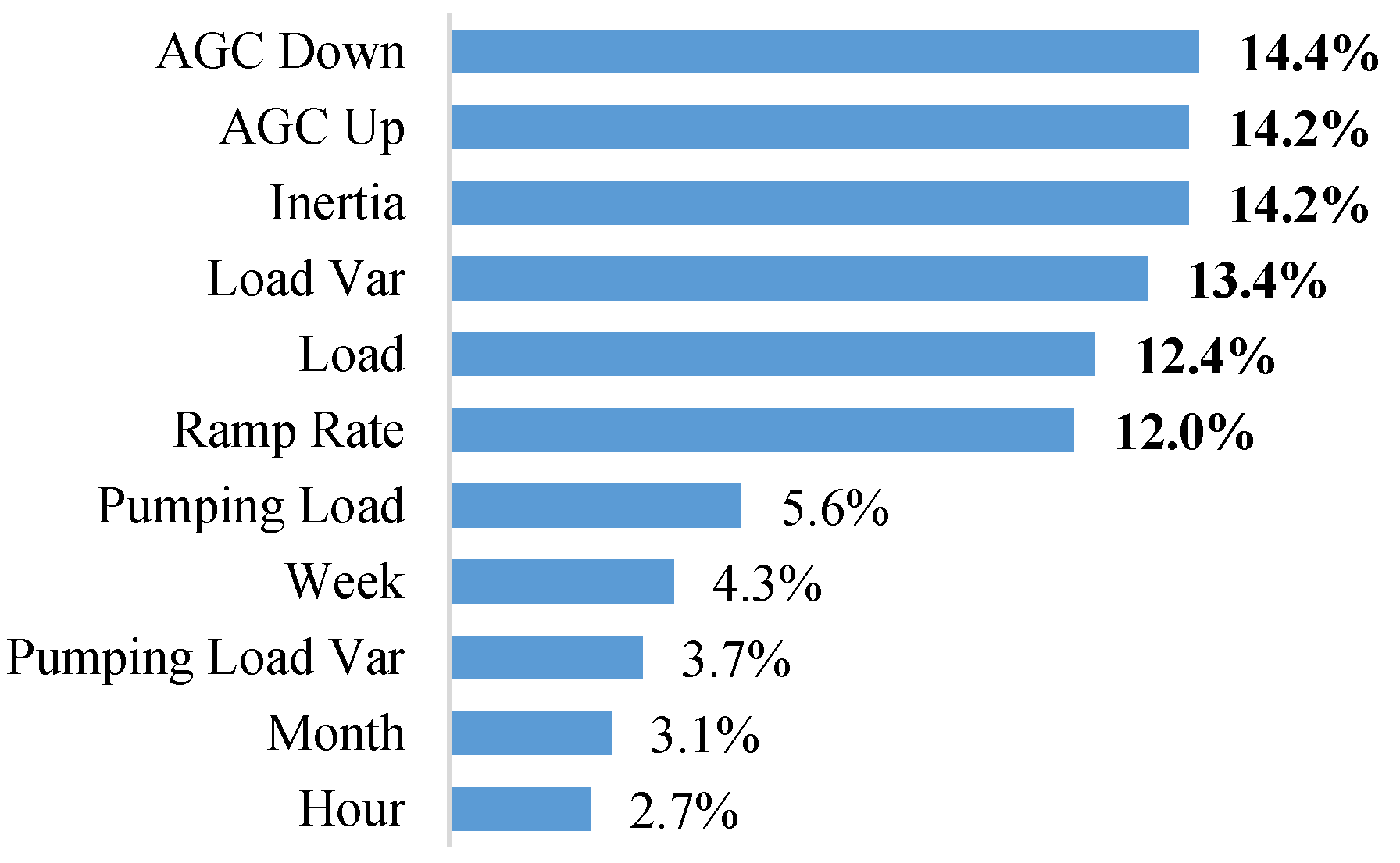
2.3. Feature Selection

Generally speaking, features presenting with a higher proportion have a greater effect on the model outcome. To extract the influential features, we introduce the ensemble learning technique.

The underlying concept of ensemble learning is to construct a single strong learner through the integration of multiple weak learners [22]. Among the many available ensemble learning techniques, gradient boosting decision tree (GBDT), which belongs to the boosting tree-based algorithms, has been suggested in this case because it can use multiple weak decision trees to construct a single strong decision tree (low variance low bias). In the implementation of GBDT, the convergence rate for the loss function is accelerated by a gradient function, and the overall deviation of the algorithm is gradually reduced as the training process proceeds [23]. After careful consideration, we decided that the analysis of the Taipower data collected in the present study did not require parallel computing, but the high prediction accuracy was a greater concern. Therefore, the GBDT algorithm was deliberately chosen for feature selection.

Figure 4a presents a schematic diagram of the GBDT procedure. In general, the GBDT algorithm consists of a decision tree (DT) structure constructed within a gradient boosting (GB) architecture. The integrated architecture ensures that the predicted value goes along the negative gradient direction to approach the actual value and minimizes the residual between the two values (i.e., the predicted value and the actual value). In the present study, the loss function of the GBDT algorithm is set as the least square error between the predicted value and the actual value, as shown in Equation (3):

$$L\left(y_i-f\left(x_i\right)\right)=\frac{1}{2}{\left[y_i-f\left(x_i\right)\right]}^2$$

(3)

where $y_i$ is the actual value. In this research, the historical CPS1 score is regarded as $y_i$, the predicted value is $f\left(x_i\right)$, and $x_i$ is the input of the ith sample. Each sample has 11 features during the feature selection procedure.

At first, the initialization of the estimated value $f_0\left(x\right)$ is set as the mean of the samples. The estimated residual ${\gamma }_{im}$ of each iteration is determined by taking the partial derivation of the loss function as shown in Equation (4). Then, the residuals of every sample are calculated by the difference between the actual value of the mth tree and the predicted value of the (m − 1)th tree. The estimated residual of the ith sample in the mth tree is calculated by

$${\gamma }_{im}=-{\left[\frac{\partial L\left(y_i,f\left(x_i\right)\right)}{\partial f\left(x_i\right)}\right]}_{f=f_{m-1}}$$

(4)

Then, a regression decision tree (RDT) is constructed to fit the estimated residual ${\gamma }_{im}$, and the terminal regions $R_{jm}$ of the decision tree are given. Note that each leaf $R_{jm}$ of a decision tree can have more than one sample ${\gamma }_{im}$. However, it is unclear what the real output value of each leaf should be if there is more than one sample in the same leaf. Therefore, the new residual ${\gamma }_{jm}$ (i.e., the value of each leaf) is calculated by the samples of the terminal leaf $R_{jm}$, as shown in Equation (5):

$${\gamma }_{jm}=\arg {\min }_{\gamma }{\displaystyle \sum _{x_i\in R_{jm}}L\left(y_i,f_{m-1}\left(x_i\right)+\gamma \right)}$$

(5)

where $R_{jm}$ refers to the jth terminal region in the mth tree.

Finally, the estimated model $f_m\left(x\right)$ as shown in Equation (6) is updated according to the new residual ${\gamma }_{jm}$ and the learning rate $\alpha$:

$$f_m\left(x\right)=f_{m-1}\left(x\right)+\alpha {\displaystyle \sum _{j=1}^{Jm}{\gamma }_{jm}I\left(x_i\in R_{jm}\right)}$$

(6)

The entire GBDT procedure is completed according to a set number of iterations (i.e., the number of decision trees M) [24]. For this case, the process deals with 120,000 data samples. Among the collected inliers, 70% were taken as the training set, with the remainder used for testing. To avoid over-fitting, the training set was used to train the model using five-fold cross-validation. After finishing all settings of the grid search, the best result was obtained in the 200th iteration, with the main hyperparameters of the model, namely the learning rate and the depth of the regression tree, having values of 0.08 and 9, respectively.

From the results of the feature selection, the importance of all frequency-sensitive features with CPS1 score are ranked and shown in Figure 5. Figure 5 shows the GBDT results for the relative importance of the 11 features in the CPS1 model. The percentage of each feature indicates the associated number of nodes over the whole decision tree that is shown in Figure 4b. The highest six features, namely AGC down, AGC up, inertia, load variation, load, and ramp rate, account for 80% of the total number of nodes. In other words, these features have greater influence on the CPS1 score. It is interesting to note that the dispatchers originally felt that the amount of pumped-storage load could be an important factor that affected the CPS1 quality. However, the result of Figure 5 shows that the influence of the pumped-storage load was not as high as they expected. Consequently, the frequency-sensitive features that have higher percentage weightings in the rank are selected to construct the FRM model.

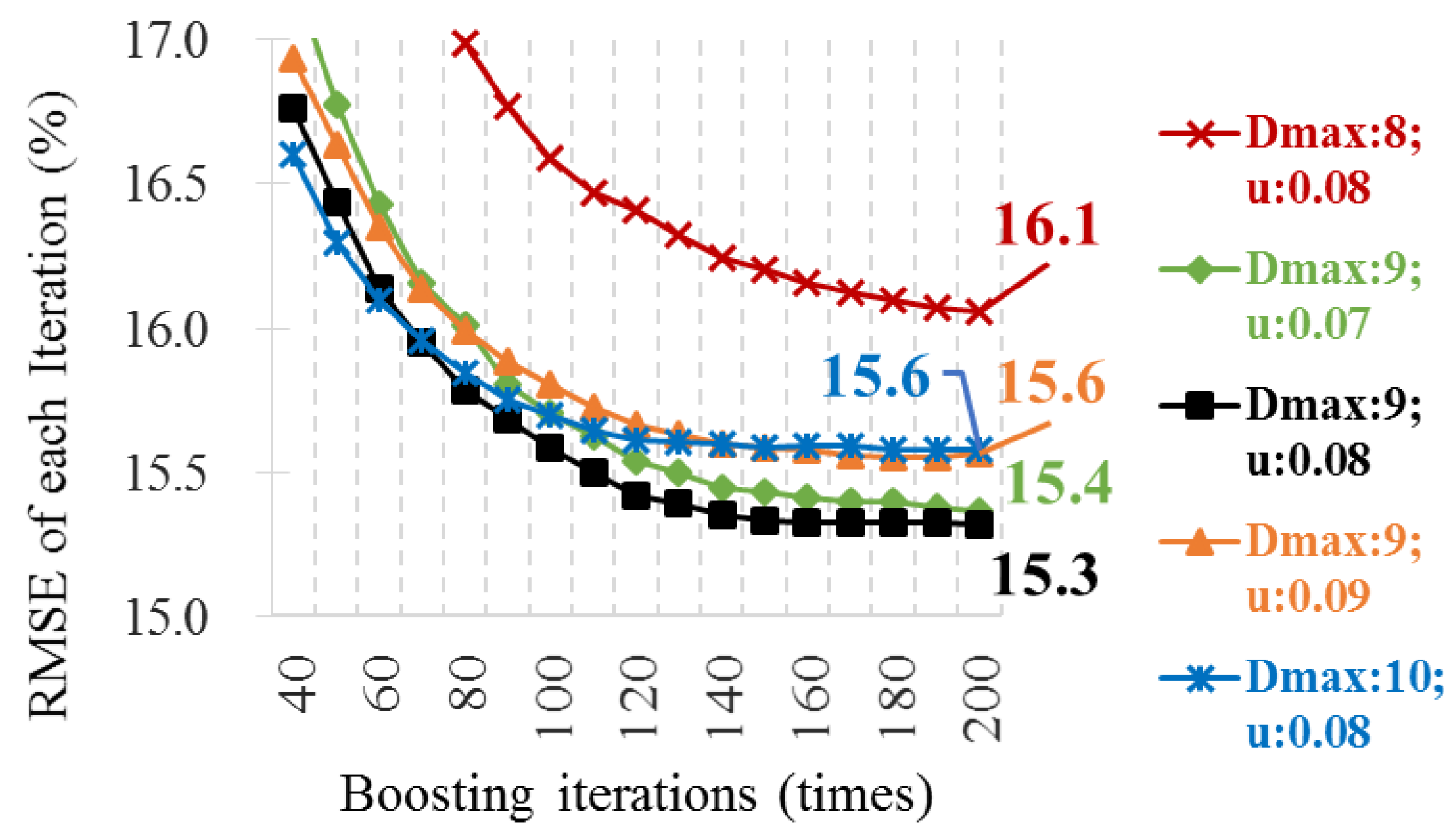
2.4. CPS1 Model Construction

To reduce the data dimensionality and data processing complexity, only the first six features in Figure 5 were selected to construct the CPS1 model, i.e., the FRM model. The method of constructing the CPS1 model was the same as the method of feature selection described in Section 2.3. The hyperparameters of the CPS1 model were once again adjusted using the grid search method and the five-fold cross-validation.

Figure 6 shows the variation of the root mean square error (RMSE) of the CPS1 model with the number of iterations as a function of the depth and learning rate. The optimal model performance was obtained using a learning rate of 0.08 and a tree depth of 9. It is seen that for a constant learning rate u, a simple model with a lower depth (e.g., a tree depth, dmax, equal to 8) leads to under-fitting compared to the optimal solution (dmax = 9, u = 0.08). By contrast, a complex model with greater depth (e.g., dmax = 10) converges rapidly during the first 60 iterations, but reaches the minimum RMSE value only much later. The average RMSE of the training set and testing set were equal to 15.3% and 17.2%, respectively.

3. UC Optimization Program for the Taipower System

The generation mix of the Taipower system in 2015 was roughly 76% fossil-fueled, 11% nuclear, 5% pumped-storage hydro, 4% cascading hydro, 3% PV generation, and 1% other renewable resources [25]. To feature different generating units for complying with the unit dispatch constraints. A systematic UC model was constructed using the general algebraic modeling system (GAMS). This UC model comprised 118 generating units, including nuclear, coal, combined-cycle, diesel, heavy oil, hydro cascade, and pumped-storage units. The original aim of the model was to minimize the total system cost (comprising the fuel cost, the minimum output cost, the start-up cost, and the ancillary service cost) by performing peak load shifting of the load curve. Having constructed the model with around 140,000 equations, the UC problem was solved using the mixed integer linear programming (MILP) method of the Gurobi solver.

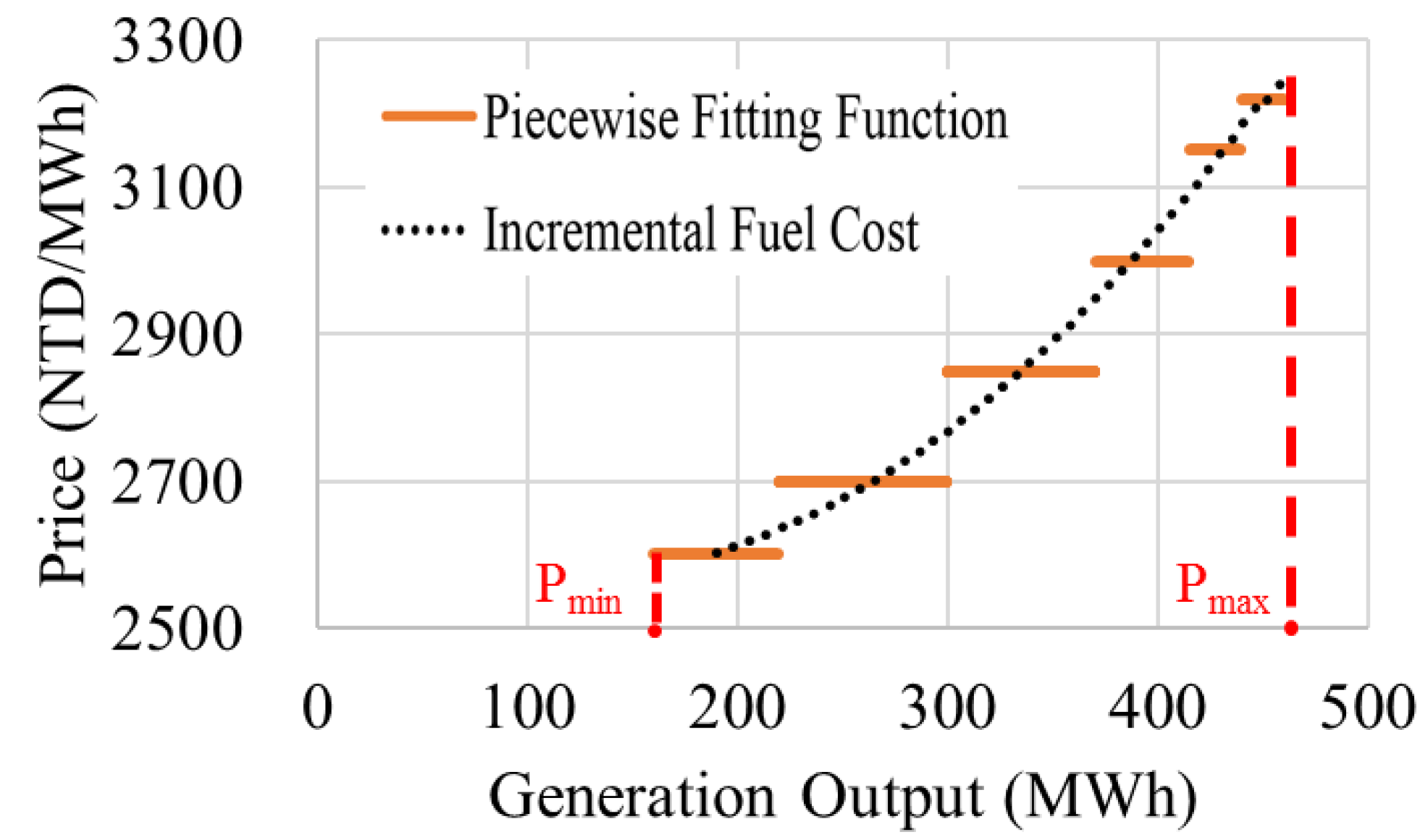
3.1. Objective Function

The objective function was designed to minimize the total cost of thermal units in the whole Taipower system. The total cost includes the incremental fuel cost, minimum level cost, hot/warm/cold start-up cost and the penalty of the power shortage. In order to construct the linearized UC model, the incremental fuel cost of each unit is fitted by six piecewise functions. An example of the incremental fuel cost with the piecewise fitting function is depicted in Figure 7 and the total cost function is described in Equation (7):

$$\begin{array}{cc}TotalCost=& {\displaystyle \sum _G{\displaystyle \sum _{H}PminCos{t}_g\cdot U_{g,h}}}+{\displaystyle \sum _G{\displaystyle \sum _H{\displaystyle \sum _S{P}_{g,h,s}\cdot tp\cdot Pric{e}_{g,h}^E}}}+{\displaystyle \sum _{H}Slac{k}_h^E\cdot Penalt{y}^E}\hfill \\ & +{\displaystyle \sum _{H}Slac{k}_h^{AGCUp}\cdot Penalt{y}^{AGCUp}}+{\displaystyle \sum _{H}Slac{k}_h^{AGCDown}\cdot Penalt{y}^{AGCDown}}\hfill \\ & +{\displaystyle \sum _G{\displaystyle \sum _H{S}_{g,h}^{hot}\cdot SuCos{t}_{g,h}^{hot}}}+{\displaystyle \sum _G{\displaystyle \sum _H{S}_{g,h}^{warm}\cdot SuCos{t}_{g,h}^{warm}}}+{\displaystyle \sum _G{\displaystyle \sum _H{S}_{g,h}^{cold}\cdot SuCos{t}_{g,h}^{cold}}}\hfill \end{array}$$

(7)

where PminCost_g is the cost of the scheduled power generation of each unit $g$ at minimum level [unit: New Taiwan Dollar, NTD]; $U_{g,h}$ is the status of each traditional generator $g$ in the period $h$,$h\in \left\{1,2,\dots ,H\right\}$; $tp$ is the time period in UC [in hour]; $P_{g,h,s}$ is the scheduled power generation of each segment $s$ of each unit $g$ in period $h$ [unit: MW]; $Pric{e}_{g,h,s}^E$ is the fuel cost of each segment $s$ of each unit $g$ in period $h$ [unit: NTD/MWh]; $Slac{k}_h^E, Slac{k}_h^{AGCUp}, Slac{k}_h^{AGCDown}$ are the slack factor of the requirement for energy, AGC Up reserve and AGC Down reserve in period $h$, respectively [unit: MW]; $Penalt{y}^E, Penalt{y}^{AGCUp}, Penalt{y}^{AGCDown}$ are the penalty price for shortage of energy, AGCUp reserve and AGCDown reserve in period $h$, respectively [unit: NTD/MW]; $S_{g,h}^{hot}, S_{g,h}^{warm}, S_{g,h}^{cold}$ are the hot, warm and cold start-up status of each unit $g$ in period $h$; $SuCos{t}_{g,h}^{hot}, SuCos{t}_{g,h}^{warm}, SuCos{t}_{g,h}^{cold}$ are the cost of each unit $g$ for hot, warm and cold start-up status in period $h$, respectively [unit: NTD].

3.2. UC Constraints

The constraint of balancing requirements of supply-side and demand-side is shown as Equation (8), the constraints of unit characteristics are shown as Equations (9)–(19) and the reservoir-related constraints are shown as Equations (20) and (21).

(i)

The balancing requirement of supply-side and demand-side considering the PSHU:

$$Loa{d}_h+{\displaystyle \sum _G{P}_{g,h}^{PSHUp}}\cdot tp=\left({\displaystyle \sum _G{P}_g^{\min }\cdot U_{g,h}}+{\displaystyle \sum _G{\displaystyle \sum _S{P}_{g,h,s}}}\right)\cdot tp+{\displaystyle \sum _G{P}_{g,h}^{PSHUg}}\cdot tp+Slac{k}_h^E$$

(8)

where $Loa{d}_h$ is the load requirement in period $h$ [unit: MWh]; $P_{g,h}^{PSHUp}$ is the scheduled pumping load of PSHU [unit: MW]; $P_{g,h}^{PSHUg}$ is the scheduled power generation of PSHU [unit: MW]; $P_g^{min}$ is the minimum output limit of each unit $g$ [unit: MW].

(ii)

The upper and lower limits of units including thermal, hydro and PSHU:

$$P_g^{\min }\cdot U_{g,h}\le P_g^{\min }\cdot U_{g,h}+{\displaystyle \sum _S{P}_{g,h,s}}\le P_g^{\max }\cdot U_{g,h}$$

(9)

where $P_g^{max}$ is the maximum output limit of each unit $g$ [unit: MW].

(iii)

The ramp up/down limit of units:

$${\displaystyle \sum _S{P}_{g,h,s}}-{\displaystyle \sum _S{P}_{g,h-1,s}}\le R{R}_g$$

(10)

$${\displaystyle \sum _S{P}_{g,h-1,s}}-{\displaystyle \sum _S{P}_{g,h,s}}\le R{R}_g$$

(11)

where $R{R}_g$ is the ramp rate supplied by unit $g$ in period $h$ [unit: MW/min].

(iv)

The states of start-up and shut down of units:

$$S{u}_{g,h}-S{d}_{g,h}=U_{g,h}-U_{g,h-1}$$

(12)

$$S{u}_{g,h}+S{d}_{g,h}\le 1$$

(13)

where $S{u}_{g,h}$ is the start-up status of each traditional generator $g$ in the period $h$; $S{d}_{g,h}$ is the shut down status of each traditional generator $g$ in the period $h$.

(v)

The minimum up/down time constraints of units

$${\displaystyle \sum _{t=h-M{U}_g+1}^{h}S{u}_{g,t}}\le U_{g,h}$$

(14)

$${\displaystyle \sum _{t=h-M{D}_g+1}^{h}S{d}_{g,t}}\le 1-U_{g,h}$$

(15)

where $M{U}_g$ is the must up time period of each traditional generator $g$ [unit: hour]; $M{D}_g$ is the must down time period of each traditional generator $g$ [unit: hour].

(vi)

Maximum start-up times per day:

$${\displaystyle \sum _{g}S{u}_{g,h}}\le MD{S}_g$$

(16)

where $MD{S}_g$ is the maximum start-up time of each traditional generator $g$ per day.

(vii)

Hot/warm/cold start-up:

$$S_{g,h}^{hot}+S_{g,h}^{warm}+S_{g,h}^{cold}=S{u}_{g,h}$$

(17)

$${\displaystyle \sum _{t=h-T_g^{hw}}^{h-1}S{d}_{g,t}}\ge S_{g,h}^{hot}$$

(18)

$${\displaystyle \sum _{t=h-T_g^{wc}}^{h-T_g^{hw}-1}S{d}_{g,t}}\ge S_{g,h}^{warm}$$

(19)

where $T_g^{hw}$ is time interval between hot start-up and warm start-up of each traditional generator $g$; $T_g^{wc}$ is time interval between warm start-up and cold start-up of each traditional generator $g$.

(viii)

The efficiency of the conversion of PSHU:

$${\displaystyle \sum _G{\displaystyle \sum _H\left(P_{g,h}^{PSHUg}\cdot tp\right)}}={\displaystyle \sum _G{\displaystyle \sum _H\left(P_{g,h}^{PSHUp}\cdot tp\right)}}\cdot {\eta }_g^{PSHU}$$

(20)

where ${\eta }_g^{PSHU}$ is the conversion efficiency of each PSHU generator $g$.

(ix)

The reservoir model for PSHU:

$$Q_{res,h}^{level}=Q_{res,h-1}^{level}-{\displaystyle \sum _G\left(P_{g,h-1}^{PSHUp}\cdot tp\right)/{\rho }_g}+{\displaystyle \sum _G\left(P_{g,h-1}^{PSHUg}\cdot tp/{\eta }_g^{PSHU}\right)}/{\rho }_g$$

(21)

where $Q_{res,h}^{level}$ is the water level of each reservoir [unit: m³]; ${\rho }_g$ is the electric-water ratio [unit: MWh/m³].

3.3. Addional Frequency Control Constraints

Among the selected features, AGC up, AGC down, inertia, and ramp rate are more capable of being controlled by the generating side management and are thus named as the frequency-sensitive features that could be implemented inside the UC program. In this study, the constraints of the frequency control between the supply and demand of the power system included not only the load requirement and power generation of all the units in the whole system, but also the PSHU pumping load [26,27,28,29]. The frequency control requirements specified by the CPS1 model would be incorporated into the UC model to ensure the model output was CPS1-compliant. The following paragraphs describe the inertia, AGC up, AGC down, and ramp rate constraints imposed on the UC solution by the CPS1 model.

The total inertia of the system was composed of the power generation side and the load demand side. In the actual condition, the inertia of the load demand side could not be controlled. However, the inertia of the power generation side can be obtained from the installed capacity and the inertia of the scheduling results, as shown in Equation (22). Note that $I_h^{Req}$ is the required inertia of the system in each period and is obtained directly from the CPS1 model. As the installed capacity of the generators increases, the inertia also increases. The UC optimization program selects the most suitable units by meeting the system inertia requirement and minimizing cost in every period. Thus:

$$\frac{{\displaystyle \sum _{G}MV{A}_g\cdot I_g\cdot U_{g,h}}}{{\displaystyle \sum _{G}MV{A}_g\cdot U_{g,h}+M{W}_h^{\mathrm{Renew}}}}\ge I_h^{\mathrm{Req}}$$

(22)

where $MV{A}_g$ is the capacity of each traditional generator $g$ and has units of MW,$g\in \left\{1,2,\dots ,G\right\}$; $M{W}_h^{Renew}$ is the power generation of renewables that do not contribute to system inertia in each hour; $I_g$ is the inertia of each traditional generator $g$.

In addition to the system inertia, the system frequency is also affected by the AGC up, AGC down, and ramp rate features. The AGC up capacity that each unit can supply in each period is described by Equations (23) to (25) below. Depending on the characteristics of each unit, if a unit intends to supply the full AGC up capacity, it must first be already committed and within AGC high, as shown in Equation (23). According to Taipower’s operation rules, the available AGC up capacity must be less than or equal to the ramp rate over a three-minute period, as shown in Equation (24). Finally, the total AGC up capacity provided by all the units must be greater than the total requirement given by the CPS1 model in each period, as shown in Equation (25).

$$P_g^{\min }\cdot U_{g,h}+{\displaystyle \sum _S{P}_{g,h,s}}+AGCU{p}_{g,h}\le P_g^{\max }\left(U_{g,h}-U_{g,h}^{AGC}\right)+AG{C}_g^{High}\cdot U_{g,h}^{AGC}$$

(23)

$$AGCU{p}_{g,h}\le R{R}_g\cdot 3\cdot U_{g,h}^{AGC}$$

(24)

$${\displaystyle \sum _{G}AGCU{p}_{g,h}}+Slac{k}_h^{\mathrm{AGCUp}}\ge AGCU{p}_h^{\mathrm{Req}}$$

(25)

where $AGCU{p}_{g,h}^{Acp}$ is the scheduled quantity of AGC up of each unit $g$ in period $h$ [unit: MW]; $AG{C}_g^{High}$ is the maximum limit of the AGC range of each unit $g$ [unit: MW]; $U_{g,h}^{AGC}$ is the status of the AGC mode of each unit $g$ in period $h$.

The AGC Down capacity provided by a unit stabilizes the fluctuation of the system frequency and is described by Equations (26) to (28). As shown in Equations (26)–(28), the AGC Down capacity falls between the set point and the AGC low limit of the unit, and must be less than the ramp rate over three minutes, as shown in Equation (26):

$$P_g^{\min }\cdot U_{g,h}+{\displaystyle \sum _S{P}_{g,h,s}}-AG{C}_g^{\mathrm{Low}}\cdot U_{g,h}^{\mathrm{AGC}}\ge AGCDow{n}_{g,h}$$

(26)

$$AGCDow{n}_{g,h}\le R{R}_g\cdot 3\cdot U_{g,h}^{AGC}$$

(27)

$${\displaystyle \sum _{G}AGCDow{n}_{g,h}}+Slac{k}_h^{\mathrm{AGCDown}}\ge AGCDow{n}_h^{\mathrm{Req}}$$

(28)

where $AG{C}_g^{Low}$ is the minimum limit of the AGC range for each unit $g$ [unit: MW].

The ramp rate of the parallel units in the system also exerts an impact on the CPS1 score (see Table 1). In the UC model, the total ramp rate of the committed units is constrained by the following ramp rate requirement determined by the CPS1 model:

$${\displaystyle \sum _{G}R{R}_g}\cdot U_{g,h}^{AGC}\ge R{R}_h^{\mathrm{Req}}.$$

(29)

3.4. Network Security Constraint

The network security constraint is to ensure system’s load generation balance in UC, while the line flow limit is also satisfied in the N-1 case. The network topology was built by PSS/E software including the transmission line of the voltage levels on 161 kV and 345 kV (around 1200 lines). For further details, please refer to [30,31]. The network security constraint is defined as follows:

$${\displaystyle \sum _G\left[\left(P_g^{\min }\cdot U_{g,h,k}+{\displaystyle \sum _S{P}_{g,h,s,k}}\right)\cdot ShiftFacto{r}_{g,h,k}\right]}\le LineFlowLimi{t}_{h,k}$$

(30)

where $P_g^{min}$ is the minimum output limit of each unit $g$ [unit: MW]; $U_{g,h,k}$ is the status of each generator $g$ in the period $h$,$h\in \left\{1,2,\dots ,H\right\}$ in kth case; $P_{g,h,s,k}$ is the scheduled power generation of each segment $s$ of each unit $g$ in period $h$ in kth case [unit: MW]; $ShiftFacto{r}_{g,h,\mathrm{k}}$ is the sensitivity of the line flows in the period $h$,$h\in \left\{1,2,\dots ,H\right\}$ in kth case regarding the change of. $ShiftFacto{r}_{g,h,\mathrm{k}}$ is calculated by the power flow in PSS/E; $FlowLimi{t}_{h,\mathrm{k}}$ is the capacity limit of the transmission line in the period $h$,$h\in \left\{1,2,\dots ,H\right\}$ in kth case [MW].

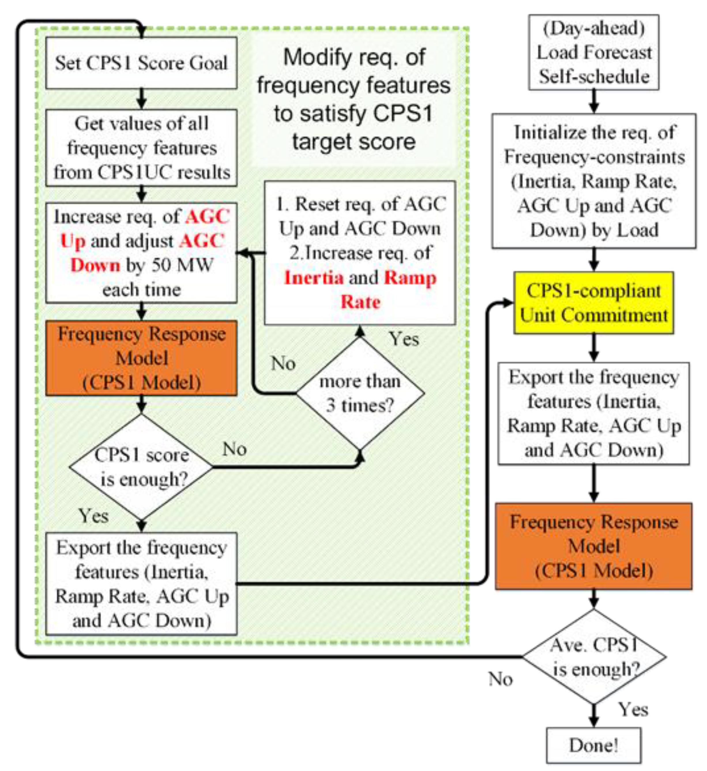
4. Integrating CPS1 Model into the UC Optimization Program

As shown in Figure 8, we integrated the UC program described above with the FRM (i.e., CPS1 model) in an iterative framework to ensure that the UC scheduling output satisfied the CPS1 target. Before executing the day-ahead UC model, we obtained the day-ahead load forecast and self-schedule information. Finally, the UC results were exported to the CPS1 model (i.e., outer loop checking) to compute the corresponding CPS1 score and to check whether the CPS1 target was achieved. If the CPS1 score could not achieve the target score, the requirements of the frequency control variables would be increased through the inner loop to satisfy the target score. Within the inner loop that is shown in the green block, additional AGC up and AGC down were called for. The updated AGC reserve would be checked again by CPS1 model (i.e., inner loop checking). If the CPS1 score still could not achieve the target score, then the requirements of inertia and ramp rate were increased (This may commit the other offline units). Note that the data resolution inside the CPS1 model is finer than that of the UC model (minute vs. hour) to closely reflect the minute-scaled LFC response.

The inertia and ramp rate quantities appear discrete in the UC model because they are related to the online generator numbers. The inertia and ramp rate quantities are accordingly adjusted after revising the AGC up and AGC down quantities. The adjustment of AGC up and AGC down quantities is more direct. That is, if the computed CPS1 score fails to meet the target score, the AGC up/down requirements are increased by 50 MW each time (see the left-hand side flowchart in Figure 8). Note that the smaller the increment of AGC up/down, the more the iterations of the UC procedure. On the other hand, the larger the increment of AGC up/down, the more the total operating cost. Consequently, a suitable increment of AGC up/down is determined, i.e., 50 MW. The renewed AGC up/down range is exported to the CPS1-compliant UC model (CPS1UC) to generate a UC solution to meet the overall constraints. If the present online units cannot fulfill the renewed AGC up/down range, the UC program calls another offline unit and updates the system ramp rate and system inertia by adding the associated unit parameters. If the target score cannot be reached in three iterations, the program directly calls another generating unit online. Finally, the frequency-sensitive features are returned to the UC model for final rescheduling.

5. Case Studies

According to NERC’s rule, CPS1 score should be 100% or higher [6]. In Taiwan, Taiwan Power Company sets the goal of CPS1 score to be 120% so that the dispatchers can have more margin to deal with daily system variance. The effectiveness of the CPS1UC was evaluated using two case studies. Case I was taking the real operating data including load demand and the unit dispatch outcome by manual dispatch (MD). We compared the unit dispatch results obtained from the CPS1UC outcome with the other two model-based UC: UC combined with the reduced order load frequency control model (ROLFC-UC) [13], and UC considering the CPS1 constraint using the long short-term memory (LSTM) algorithm (LSTM-UC) [32]. The Case II was conducted on a hypothetical case in which a photovoltaic (PV) power with maximum output of 3.9 GW (accounting for 11% of the total system generation capacity) was added to the Taipower system. In this case study, the aforementioned methodologies were used to compare the difference of the dispatch outcome. The proposed method was simulated in a GAMS platform and Python environment running using an Intel Core E3-1245V5 CPU operating at 3.50 GHz with 32 GB RAM.

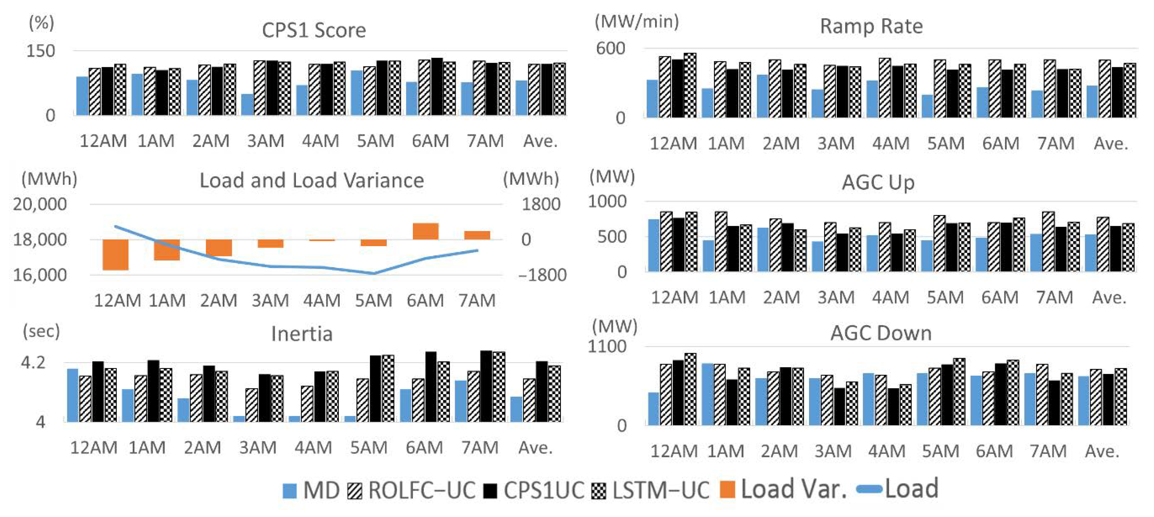
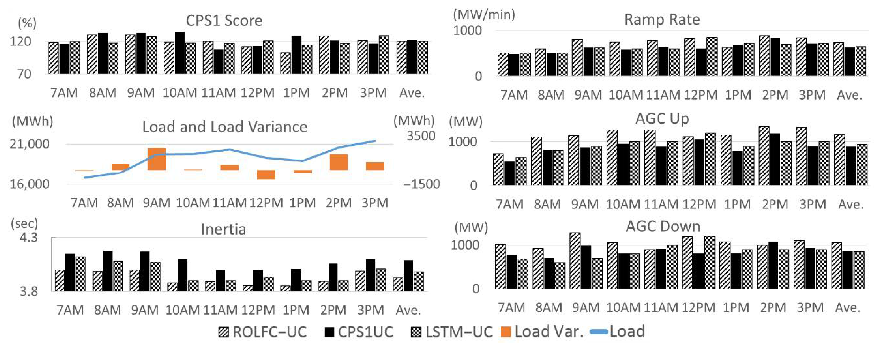
5.1. Historical Operation Case (in the Early Morning (First Shift Period))

In this case, we focus on the CPS1 enhancement for the first shift period.

Table 2. CPS1 scores and requirements of PMS and CPS1UC in the first-shift period (Averaging over eight hours).

	Manual Dispatch	ROLFC-UC	LSTM-UC	CPS1UC (Proposed)
Frequency Response Model	NaN	reduced-order LFC	LSTM (Neural Network)	GBDT (tree based)
RMSE of CPS1 on training set (%)	NaN	NaN	23.2	15.3
RMSE of CPS1 on testing set (%)	NaN	NaN	25.5	17.2
Total Operating Cost (NTD)	842 M	852 M	848 M	846 M

shows the model validation and total operating cost of the first shift period. Despite the same load demand in the testing case, the total operating costs of the individual methods are different due to the different dispatch outcomes. The accuracy of the proposed CPS1 model (i.e., RMSE 17) was better than that of the LSTM model (i.e., RMSE 25) under the model validation process. In this case, the memory usage of the LSTM is 8 times that of the GBDT. The training time of the hyperparameter tuning is 10 times that of the GBDT (GBDT took 500 s). It is evident that the tree-based ensemble learning algorithm dealing with the domain knowledge formulation is better than the LSTM.

Figure 9 shows the details of the four methods in each hour. During the load dropping period, the MD scenario shows that the operator continued to turn the generating unit off-line, resulting in low system inertia. The other problem is that the provisions of AGC reserve (AGC up and AGC down) as well as ramp rate were quite limited due to the insufficient on-line units. The sequential consequence limited system’s frequency regulation capability, resulting in low CPS1 score. Compared to the MD scenario, the remaining three methods required higher Inertia in the UC constraint, the total operating cost still maintained low among the scenarios. Note that ROLFC-UC did not take the inertia into consideration, it would need more AGC reserve (AGC up and AGC down) as well as ramp rate to keep CPS1 at 120%. On the contrary, the LSTM-UC and CPS1UC took inertia as additional UC constraint. That is the reason why these two methods came up with less regulation reserve but higher inertia requirement. Although LSTM-UC and CPS1UC led to similar results, the accuracy of the model evaluation was different.

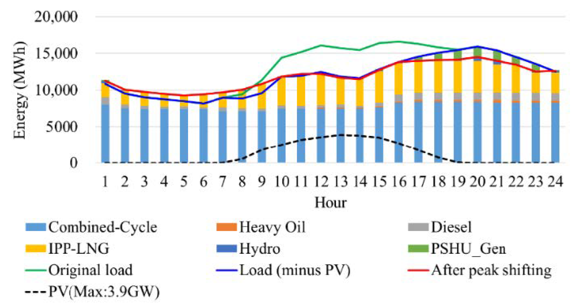
5.2. Hypothetical Case (PV Case)

In the Case II (PV Case), the load demand was the same as that in Case I but with a maximum PV power generation of 3.9 GW (accounting for 11% of the power generation of the whole system) that was assumed to be integrated into the system.

Figure 10 shows the corresponding CPS1UC scheduling results. The green curve shows the load demand. The blue curve shows the net load which is obtained by deducting the PV power generation curve (black dotted line) from the load demand curve. The net load curve shows that the original peak load was shifted from noon to evening due to the addition of PV power generation. In this case, we focus on the daytime period (from 7 a.m. to 3 p.m.) when the PV power generation was active.

Table 3. Comparisons of scheduling results by three different model-based UCs.

	ROLFC-UC	LSTM-UC	CPS1UC
Frequency Response Model (FRM)	reduced-order LFC	LSTM (neural network)	GBDT (tree-based)
RMSE of CPS1 on training set (%)	NaN	23.2	15.3
RMSE of CPS1 on testing set (%)	NaN	25.5	17.2
Total Operating Cost (NTD)	772 M	759 M	757 M

shows the cost comparison by the different three methods (i.e., ROLFC-UC vs. CPS1UC vs. LSTM-UC). Figure 11 shows that the three model-based UC all achieved the target CPS1 score. However, the values of inertia, ramp rate and AGC reserve (AGC up and AGC down) are different. The common results of these three methods show that the Inertia values during the high noon hours were lower than those during the other operating hours. The ROLFC-UC called for more AGC reserve (AGC up and AGC down) as well as ramp rate to keep CPS1 at 120% due to the lower inertia value. On the contrary, the CPS1UC and the LSTM-UC took Inertia as an additional UC constraint to keep the inertia at higher level. Therefore, they came up with less regulation reserve and ramp rate values. This case shows a trade-off between Inertia and regulation reserve, which implies that inertia is important for the frequency stability. For a power system with high penetration renewables, the unit commitment should consider not only the ramp rate and AGC reserve but inertia to ensure a good frequency quality.

6. Conclusions

This paper has proposed a model-based UC (CPS1UC) platform to ensure a CPS1-compliant unit scheduling outcome. The proposed FRM was constructed by an ensemble learning technique, the GBDT algorithm, to deal with feature identification and model training. Unlike the traditional model formulation, the ensemble learning technique help model define its own structure, tune the model parameters, and validate the model accuracy. Once the model validation is complete, the quantities of the frequency control features determined by the UC result were routinely exported to the FRM to check the CPS1 compliance until the UC result achieves the target CPS1 score. The validity and feasibility of the proposed model-based UC platform were evaluated by two case studies. In Case I, the proposed CPS1UC effectively exerted the dominant frequency control features to reach CPS1 target with less operating cost and computing resource. In Case II, system frequency becomes relatively unstable due to the increasing PV penetration into the system. To comply with the CPS1 target, it is better to maintain a certain level of system inertia. The CPS1UC solved this problem by committing several synchronous condensers and gas turbines on line. The gas turbine is more flexible to be committed in a short time and is more responsive to the frequency regulation.

As described above, the proposed FRM was constructed based on the mass historical data, the accuracy of the model could improve to reflect the most updated system as the proposed CPS1UC platform continuously operates in real time.

To sum up, the important findings of this study are listed as follows:

(1)

This study commences by formulating a set of procedures and employing an ensemble machine learning technique to analyze the real energy management system (EMS) data of an isolated power system (i.e., 118 generating units) to construct a FRM. The resulting FRM is then integrated with a UC program to determine the unit scheduling result, which minimizes the system operating cost while the frequency compliance is also maintained.

(2)

During the period of the controlled frequency with lower compliance, i.e., the early morning or high penetration RES, the system frequency quality could be improved by the proposed UC with the integration of the FRM. Testing result shows that retaining the proper quantity of frequency-sensitive feature, especially Inertia, is the most effective way to keep the high frequency quality.

(3)

The dominant features of the LFC (i.e., parameters of units, load damping, system inertia) are hard to capture. The proposed method in this paper assists dispatchers to clearly identify the frequency-sensitive features, and grasp their features effectively.

(4)

Power system frequency operation is a nonlinear and complex problem. Compare to the traditional LFC model, the proposed FRM has the advantage of self-learning by feeding in the updated inputs so that the model output is more close to the real system behavior. This feature validates the effectiveness of an artificial intelligent algorithm in a smart grid system.

References

1. Luh, P.B.; Yu, Y.; Zhang, B.; Litvinov, E.; Zheng, T.; Zhao, F.; Zhao, J.; Wang, C. Grid integration of intermittent wind generation: A Markovian approach. IEEE Trans. Smart Grid 2014, 5, 732–741. [Google Scholar] [CrossRef]
2. Su, W.; Wang, J.; Roh, J. Stochastic energy scheduling in microgrids with intermittent renewable energy resources. IEEE Trans. Smart Grid 2014, 5, 1876–1883. [Google Scholar] [CrossRef]
3. Zheng, Q.P.; Wang, J.; Liu, A.L. Stochastic optimization for unit commitment—A review. IEEE Trans. Power Syst. 2015, 30, 1913–1924. [Google Scholar] [CrossRef]
4. Zhang, N.; Hu, Z.; Dai, D.; Dang, S.; Yao, M.; Zhou, Y. Unit commitment model in smart grid environment considering carbon emissions trading. IEEE Trans. Smart Grid 2016, 7, 420–427. [Google Scholar] [CrossRef]
5. Mitani, T.; Aziz, M.; Oda, T.; Uetsuji, A.; Watanabe, Y.; Kashiwagi, T. Annual Assessment of Large-Scale Introduction of Renewable Energy: Modeling of Unit Commitment Schedule for Thermal Power Generators and Pumped Storages. Energies 2017, 10, 738. [Google Scholar] [CrossRef] [Green Version]
6. NERC Reliability Standard BAL-001-1-Real Power Balancing Control Performance. Available online: http://www.nerc.com/pa/Stand/Reliability%20Standards/BAL-001-1.pdf (accessed on 25 October 2019).
7. Ela, E.; Milligan, M.; Kirby, B. Operating Reserves and Variable Generation; NREL/TP-5500-51928; National Renewable Energy Lab (NREL): Golden, CO, USA, 2011.
8. Chung, W. Anticipatory Fuzzy Automatic Generation Control Scheme Using Very Short-Term ANN ACE Forecasting. Ph.D. Dissertation, Purdue University, West Lafayette, IN, USA, 2005. [Google Scholar]
9. Ahmadi, H.; Ghasemi, H. Security-constrained unit commitment with linearized system frequency limit constraint. IEEE Trans. on Power Syst. 2014, 29, 1536–1545. [Google Scholar] [CrossRef]
10. Pérez-Illanes, F.; Álvarez-Miranda, E.; Rahmann, C.; Campos-Valdés, C. Robust unit commitment including frequency stability constraints. Energies 2016, 9, 957. [Google Scholar] [CrossRef] [Green Version]
11. Farrokhabadi, M.; Canizares, C.; Bhattacharya, K. Unit commitment for isolated microgrids considering frequency control. IEEE Trans. Smart Grid 2018, 9, 3270–3280. [Google Scholar] [CrossRef]
12. Bao, Y.-Q.; Li, Y.; Wang, B.; Hu, M.; Zhou, Y. Day-Ahead Scheduling Considering Demand Response as a Frequency Control Resource. Energies 2017, 10, 82. [Google Scholar] [CrossRef] [Green Version]
13. Zhang, G.; McCalley, J.D. Estimation of regulation reserve requirement based on control performance standard. IEEE Trans. Power Syst. 2018, 33, 1173–1183. [Google Scholar] [CrossRef]
14. Yang, Y.; Shen, C.; Wu, C.; Lu, C. Control performance based dynamic regulation reserve allocation for renewable integrations. IEEE Trans. Sustain. Energy 2019, 10, 1271–1279. [Google Scholar] [CrossRef]
15. Ahmad, A.; Javaid, N.; Alrajeh, N.; Khan, Z.A.; Qasim, U.; Khan, A. A Modified Feature Selection and Artificial Neural Network-Based Day-Ahead Load Forecasting Model for a Smart Grid. Appl. Sci. 2015, 5, 1756–1772. [Google Scholar] [CrossRef]
16. Mujeeb, S.; Alghamdi, T.A.; Ullah, S.; Fatima, A.; Javaid, N.; Saba, T. Exploiting Deep Learning for Wind Power Forecasting Based on Big Data Analytics. Appl. Sci. 2019, 9, 4417. [Google Scholar] [CrossRef] [Green Version]
17. Mellit, A.; Pavan, A.M.; Ogliari, E.; Leva, S.; Lughi, V. Advanced Methods for Photovoltaic Output Power Forecasting: A Review. Appl. Sci. 2020, 10, 487. [Google Scholar] [CrossRef] [Green Version]
18. Moradzadeh, A.; Zakeri, S.; Shoaran, M.; Mohammadi-Ivatloo, B.; Mohammadi, F. Short-Term Load Forecasting of Microgrid via Hybrid Support Vector Regression and Long Short-Term Memory Algorithms. Sustainability 2020, 12, 7076. [Google Scholar] [CrossRef]
19. López Gómez, J.; Ogando Martínez, A.; Troncoso Pastoriza, F.; Febrero Garrido, L.; Granada Álvarez, E.; Orosa García, J.A. Photovoltaic Power Prediction Using Artificial Neural Networks and Numerical Weather Data. Sustainability 2020, 12, 10295. [Google Scholar] [CrossRef]
20. Domingues, R.; Filippone, M.; Michiardi, P.; Zouaoui, J. A comparative evaluation of outlier detection algorithms: Experiments and analyses. Pattern Recognit. 2018, 74, 406–421. [Google Scholar] [CrossRef]
21. Liu, F.T.; Ting, K.M.; Zhou, Z. Isolation Forest. In Proceedings of the 2008 Eighth IEEE International Conference on Data Mining, Pisa, Italy, 15–19 December 2008; pp. 413–422. [Google Scholar]
22. Sagi, O.; Rokach, L. Ensemble learning: A survey. Wiley Interdiscip. Rev. Data Min. Knowl. Discov. 2018, 8, e1249. [Google Scholar] [CrossRef]
23. Friedman, J. Greedy function approximation: A gradient boosting machine. Ann. Stat. 2001, 29, 1189–1232. [Google Scholar] [CrossRef]
24. Hastie, T.; Tibishirani, R.; Friedman, J. The Elements of Statistical Learning, 2nd ed.; Springer: New York, NY, USA, 2009. [Google Scholar]
25. The Architecture of Power Supply for Taipower. Available online: http://www.moeaboe.gov.tw (accessed on 12 January 2020).
26. Guan, X.; Luh, P.B.; Yan, H.; Rogan, P. Optimization-based scheduling of hydrothermal power systems with pumped-storage units. IEEE Trans. Power Syst. 1994, 9, 1023–1031. [Google Scholar] [CrossRef]
27. Alemany, J. Short-term scheduling of combined cycle units using mixed integer linear programming solution. Energy Power Eng. 2013, 5, 161–170. [Google Scholar] [CrossRef] [Green Version]
28. Huang, W.; Hu, T.; Hsu, K.; Tsai, C.; Wu, C. Analysis of simulated bidding results for ancillary services of Taiwan power system: Using thermal power plants as an example. Mon. J. Taipower’s Eng. 2014, 795, 103–110. [Google Scholar]
29. Alvarez, G.E.; Marcovecchio, M.G.; Aguirre, P.A. Security-constrained unit commitment problem including thermal and pumped storage units: An MILP formulation by the application of linear approximations techniques. Electr. Power Syst. Res. 2018, 154, 67–74. [Google Scholar] [CrossRef]
30. SIEMENS. Siemens PTI.PSS/E 35 Program Operation Manual; SIEMENS: New York, NY, USA, 2019. [Google Scholar]
31. Hui, H. Reliability Unit Commitment in ERCOT Nodal Market. Ph.D. Dissertation, University Texas, Arlington, TX, USA, 2013. [Google Scholar]
32. Chiu, H.; Lin, Y.; Chang-Chien, L.; Wu, C. Modeling of the CPS1 for the Frequency Constrained Unit Commitment. In Proceedings of the 2019 IEEE PES Asia-Pacific Power and Energy Engineering Conference (APPEEC), Macao, China, 1 December 2019; pp. 1–5. [Google Scholar]
Figure 1. Procedure of constructing a CPS1-compliance model (ALGO: algorithm).
Energies 14 00310 g001
Figure 2. CPS1 scores of the Taipower system over the whole year (2015).
Energies 14 00310 g002
Figure 3. Outlier detection results for six features.
Energies 14 00310 g003
Figure 4. The architecture of GBDT for the CPS1 model: (a) Architecture of GBDT, (b) Part of decision tree.
Energies 14 00310 g004
Figure 5. Ranking of frequency-sensitive features by importance.
Energies 14 00310 g005
Figure 6. Variation of RMSE with iteration number as a function of maximum tree depth and learning rate.
Energies 14 00310 g006
Figure 7. Piecewise fitting function of the incremental fuel cost of each unit.
Energies 14 00310 g007
Figure 8. Integration of the proposed CPS1 model with the UC program.
Energies 14 00310 g008
Figure 9. Hourly results of each scenario in the Normal Operation Case.
Energies 14 00310 g009
Figure 10. CPS1UC scheduling results with an addition of maximum 3.9 GWh PV.
Energies 14 00310 g010
Figure 11. Comparisons of scheduling results by three different model-based UCs during the daytime period.
Energies 14 00310 g011