Detailed Analytical Approach to Solve the Magnetoacoustic Tomography with Magnetic Induction (MAT-MI) Problem for Three-Layer Objects

Abstract

This paper is devoted to an analytical approach to the magnetoacoustic tomography with magnetic induction (MAT-MI) problem for three-layer low-conductivity objects. For each layer, we determined closed-form analytical expressions for the eddy current density and Lorentz force vectors based on the separation of variables method. Next, the analytical formulas were validated with numerical solutions obtained with the help of the finite element method (FEM). Based on the acoustic dipole radiation theory, the influence of the transducer reception pattern on MAT-MI was investigated. To obtain acoustic wave patterns, as a system transfer function we proposed the Morlet wavelet. Finally, image reconstruction examples for objects of more complex shapes are presented, and the influence of the MAT-MI scanning resolution and the presence of the noise on the image reconstruction quality was studied in detail.

1. Introduction

The electrical properties of biological tissues, such as the electrical conductivity or permittivity, can provide important information regarding the physiological and pathological properties; however, the accurate quantification of these physical variables for use in early medical diagnosis is still valid and challenging [1]. Recently, several noninvasive electromagnetic imaging methods were developed to determine the electrical conductivity distribution of various low-conductive objects. Among them, magnetoacoustic tomography with magnetic induction (MAT-MI) was recently established [2], which overcomes the unwanted shielding effect occurring in electrical impedance tomography (EIT), magnetoacoustic tomography with current injection (MAT-CI) [3], and magneto-acoustic tomography (MAT) [4,5,6] as well as defeats the problem of low spatial resolution of magnetic induction tomography (MIT) [7]. The MAT-MI technique—as a multiphysics imaging approach—is based on the coupling of electromagnetism and ultrasound into one hybrid method. Such a combination limits the main drawbacks of previous imaging modalities [8,9,10]. In the last years several variants of such a tomographic technique are being explore. However, the occurrence of this physics phenomena still require careful scientific study in a quantitative way [11,12,13]. In particular, analytical and numerical calculations can provide new and important information about the nature of the electromagnetic-acoustic phenomenon [14,15,16,17,18,19]. The literature on the subject is extensive and the cited references should only be treated as representative examples.

In general, the MAT-MI method can be divided in two main parts. The former, the so-called forward problem, comes down to expressing the acoustic pressure generated in a biological tissue or any other low-conductivity object. The latter, called the inverse problem, is based on reconstructing the source of the ultrasonic waves according to the electrical signals collected by sensors. In the past, several reconstruction algorithms have been applied. The most common approach is based on using various back-projection algorithms and time-reversal methods, which assume a lossless and acoustically homogenous medium [2,11,12]. For a more accurate reconstruction, the algorithms must focus on the real conditions of the MAT-MI system. Recently, a new two-dimensional inverse algorithm of electrical conductivity distribution imaging was also proposed that, by analysing singular values in the system matrix MAT-MI model, couples the distribution of the conductivity with ultrasound signals [20].

In this paper, for the first time we present a detailed step-by-step analytical approach to solve the MAT-MI problem for three-layer objects. For each layer, we determined closed-form analytical expressions for the eddy current density and Lorentz force vectors. The analytical solutions were validated with those obtained using Comsol Multiphysics software (Comsol, Burlington, MA, USA) based on the finite element method (FEM). Next, based on the acoustic dipole radiation theory [21,22], the influence of the transducer reception pattern on MAT-MI was investigated, and, to obtain acoustic wave patterns, as the system transfer function the real- and imagine-valued Morlet wavelets were used [23,24]. In the last chapter, the image reconstruction examples for objects of more complex shapes and additionally in the presence of the noise are presented and analyzed. The impact of the MAT-MI scanning resolution on the image reconstruction quality was studied in detail. This problem has never been fully considered in the past, as in this article. Although similar problems were analyzed, either the authors did not quantify the details of eddy currents and Lorentz forces, or the objects’ shapes or number of layers were different [6,8,9,11,12,13,14,15,16,17,18,19,21,22,25].

2. Principles of MAT-MI

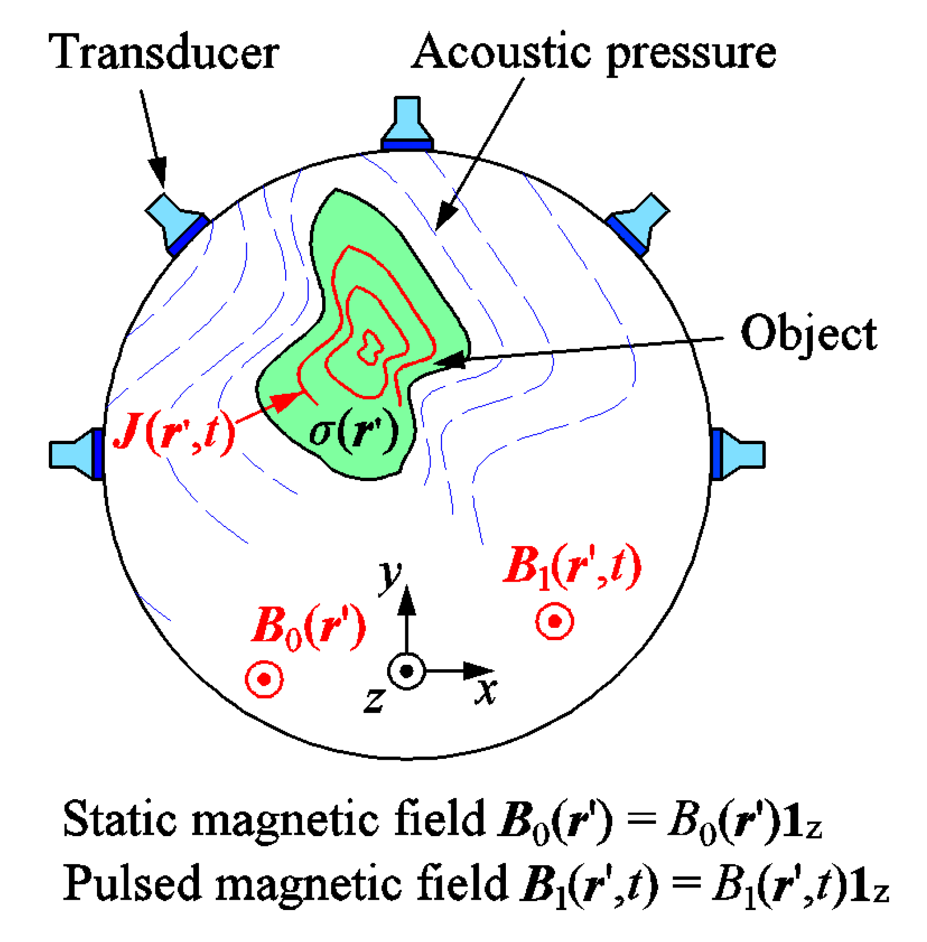
The MAT-MI method is illustrated in Figure 1. A conductive object to be imaged with conductivity σ(r’) (r’ is the position vector) is placed in both external static B₀(r’) and time-varying (pulsed) B₁(r’, t) (t is time) magnetic fields. The static and pulsed magnetic fields are assumed to cover the whole object with the surrounding area. The pulsed magnetic field induces eddy currents in the whole object’s volume. The eddy current density spatial and time distribution J(r’, t) is determined by the B₁ field and the conductivity σ(r’) distribution inside the object under test. We also assumed that, in the MAT-MI system, a MHz pulsed magnetic field is used, and thus the conduction current is much greater than the displacement current. Therefore, the electromagnetic induction problem can be considered as quasi-static, and finally the tissue capacitance effect related to permittivity will be further ignored.

Interactions between the static magnetic field and the induced eddy currents produce the Lorentz force and generate detectable acoustic signals, which can be acquired by a set of piezoelectric transducers. In the last stage, using various back-projection methods, the recorded ultrasonic signals are used to reconstruct the object’s conductivity map [26].

The forward problem concerns the acoustic signal generation mechanism of MAT-MI. This phenomenon includes two physical processes, electromagnetic induction in the conducting object and acoustic wave propagation coupled with the Lorentz force. The magnetic stimulation B₁(r’, t) may be expressed by the infinitesimal circulation of its magnetic vector potential A(r’, t): B₁(r’, t) = ∇ × A(r’, t). The small value of electrical conductivity means that the secondary magnetic field effect can be ignored, so we can assume that A(r’, t) ≈ A_p(r’, t), where A_p(r’, t) denotes the original vector potential induced by excitation the coil in case of the lack of the object.

The electric field and the eddy current density vectors inside the object can be described as follows [2,3,4,6,7,8,11,12,13,14,15,16,17]:

$$\begin{array}{cc}E(r^{\prime },t)=\frac{-\partial A(r\prime ,t)}{\partial t}-\nabla V(r^{\prime },t),& J(r^{\prime },t)=\sigma (r^{\prime })E(r^{\prime },t)\end{array},$$

(1)

where V(r’, t) is the electric scalar potential.

In case of a sufficiently short pulse, after splitting the temporary magnetic field for the functions of space and time, the Lorentz force density can be expressed as [2,3,4,6,7,8,11,12,13,14,15,16,17]:

$$F(r^{\prime },t)=\left[J\left(r^{\prime }\right)\times B_0\left(r^{\prime }\right)\right]\delta \left(t\right),$$

(2)

where δ(t) is the Dirac delta function in the time domain.

In the MAT-MI, the divergence of the force arising from (2) leads to ultrasonic vibrations and produces a mechanical wave resulting from the following wave equation [2,3,4]:

$${\nabla }^{2}p(r^{\prime },t)-\frac{1}{c_s^2}\frac{{\partial }^{2}p(r\prime ,t)}{\partial t^2}=\nabla \cdot \left[J\left(r^{\prime }\right)\times B_0\left(r^{\prime }\right)\right]\delta \left(t\right),$$

(3)

where p(r’, t) is the ultrasonic pressure at the point r’ in space, c_s = (ρ₀∙β_s)^−1/2 is the ultrasonic speed, ρ₀ and β_s are the density and the adiabatic compressibility of the medium, respectively.

Using Green’s function, Equation (3) can be solved as [2,3,4,6,7,8,11,12,13,14,15,16,17]:

$$p(r^{\prime },t)=\frac{-1}{4\mathsf{\pi }}{\displaystyle \underset{V}{\int }{\nabla }_{r^{\prime }}\cdot \left[J\left(r^{\prime }\right)\times B_0\left(r^{\prime }\right)\right]\frac{\delta \left(t-\frac{R}{c_s}\right)}{R}}\mathrm{d}{r}^{\prime },$$

(4)

where r defines the transducer position, R = |r − r’|, and the integration is performed over the entire volume of the sample containing the object and medium.

The complete MAT-MI inverse problem comes down to reconstructing the conductivity distribution map σ(r’) of the object’s volume by using the acoustic pressure measurements. In principle, the inverse problem can be split into two main steps. First, the references term ∇·(J × B₀) of the wave equation may be reproduced using the time-reversal method. The general idea of the time-reversal method is that the ultrasonic wave propagation can be inverted in time and played back. This method can be used to every effect described by the so-called time-reversal-invariant equations. The time-reversal technique usually consists of two parts. At the beginning, an ultrasonic pressure p(r’, t) is produced by a source (in experiments or in simulations). This ultrasonic pressure is either acquired by transducers located circumferentially (as shown in Figure 1) or computed at so-called ‘measuring points’ as a function of time and collected. If all the stored signals are reverted in time and reemitted from the location where they were recorded, the resultant ultrasonic waves will converge back to the point where it was originally transmitted. The time of this recording is given by T. Next, the calculations at each position are reverted in time, which results in the time-reverted signals [14,21,22,26]:

$$p_{TR}\left(r,t\right)= p\left(r,T-t\right) .$$

(5)

During the reconstruction process, we assume that the studies are ideal, i.e., the medium is lossless and acoustically homogenous, and the recorded signals are noise-free. In the second part, the measured points are utilized as sources where the time-reverted pressure pulses p_TR are applied deployed together. The resultant waves travel back through the object and interfere constructively at the location of the primary source. Using the time-reversal method, the ultrasonic source can be characterized as follows [2,3,4,6,7,8,14,21,22,26]:

$$\nabla \cdot \left[J\left(r^{\prime }\right)\times B_0\left(r^{\prime }\right)\right]\approx \frac{1}{2\mathsf{\pi }{c}_s^3}{\displaystyle \underset{S_d}{\int }{\frac{\mathit{n}\cdot (r-r_d)}{{\left|r-r_d\right|}^2}\frac{{\partial }^{2}p\left(r_d,t\right)}{\partial t^2}|}_{t=\left|r-rd\right|/c_s}}\mathrm{d}{S}_d,$$

(6)

where r_d is the detection point on the surface S_d, and n is a unit vector normal to the surface S_d at r_d.

In the latter step, the conductivity decomposition σ(r’) is reproduced from ∇·[J(r’) × B₀(r’)]; however, this is not a trivial task. To solve this problem, a number of methods have recently been presented. For instance, the method proposed in [2] relies on changing the direction of the static magnetic field B₀, while in [11], the authors presented a reconstruction technique based on piecewise distribution. One of the last approaches is based on the assumption that the MAT-MI inverse problem is treated as an ill-conditioned inverse problem, similarly to the case of EIT and MIT tomographies [20].

3. Analytical Solutions for Transient Eddy Currents in Three-Layer Cylindrical Objects

The analytical formulas, obtained for one- or two-dimensional arrangements, are widely used in electromagnetism, although they can only refer to highly idealized cases. Nevertheless, the careful examination of electromagnetic induction in low-conductivity objects is highly significant, because the results obtained affect the next steps in the tomographic process of image reconstruction. For more complex shapes, only the numerical procedures, e.g., FEM, can be applied [6,9,10,13,14,15,16,17].

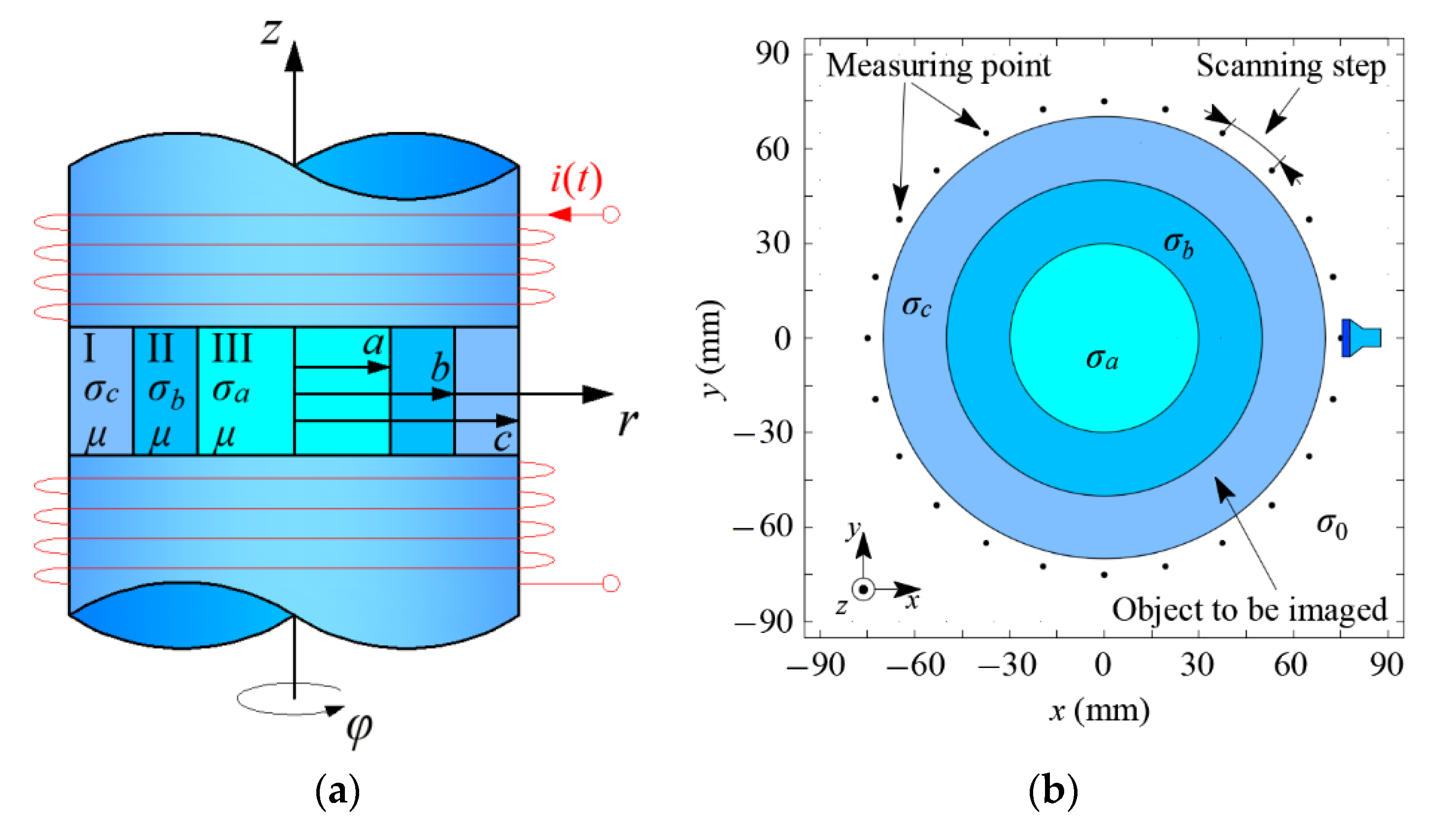
Considering the Cartesian coordinate system (x, y, z), we supposed that the structure to be reconstructed, the static B₀(r’) and pulsed B₁(r’, t) magnetic fields are homogeneous in the direction of the z-axis. In such a case, the resulting, induced eddy current density vector J(r’, t) is bounded in the xy plane. Hence, in this problem, the 3D MAT-MI forward model can be reduced as a two-dimensional problem with non-homogeneous conductivity pattern σ(r’) placed in the xy (z = 0) plane for a current magnetic excitation.

Let us consider a long three-layer conducting circular cylinder, which, in general, can correspond to a typical three-layer biological tissue with constant electrical conductivities σ_a, σ_b, and σ_c in each layer and magnetic permeability μ placed in a magnetic field H (B = µH) generated by current i(t) flowing in a winding coil that tightly surrounds the cylinder. The problem is shown schematically in Figure 2. The current i(t) is described by the step function, i.e., i(t) = I₁1(t), which consequently makes the emerging magnetic field around the cylinder, which can be expressed as: H(t) = (nI₁/l)1(t)1_z = H₁1(t)1_z, n—the number of turns, and l—the length. Considering the cylindrical coordinate system (r, φ, z), the three different conductivities designate the following calculation regions: I (b ≤ r ≤ c), II (a ≤ r ≤ b), and III (0 ≤ r ≤ a), with conductivities σ_c, σ_b, and σ_a, respectively.

There is only an axial component H = H(r, t)1_z of the magnetic field inside the cylindrical object. After introducing the cylindrical coordinate system (r, φ, z), the following partial differential equation must be fulfilled [14,15,16]:

$$\frac{{\partial }^{2}H}{\partial r^2}+\frac{1}{r}\frac{\partial H}{\partial r}=\left\{\begin{array}{c}\begin{array}{cc}\mathrm{I}:& {\sigma }_c\end{array}\\ \begin{array}{cc}\mathrm{II}:& {\sigma }_b\end{array}\\ \begin{array}{cc}\mathrm{III}:& {\sigma }_a\end{array}\end{array}\right\}\mu \frac{\partial H}{\partial t}$$

(7)

with the initial and boundary conditions:

$$H\left(r,0\right)=0 \mathrm{for} r\in \langle 0,c);H\left(c,t\right)=H_1 \mathrm{for} t>0;\underset{t\to \infty }{\lim }H\left(r,t\right)=H_1 \mathrm{for} t>0;$$

The derivation method of the expressions for current density vector is detailed in Appendix A. Taking into account that J = ∇ × H (the displacement current density vector is neglected), the eddy current density vector has only an angular component J = J(r, t)1_φ, and the mathematical expressions in each region can be determined as follows:

$$\{\begin{array}{l}{J}_{\mathrm{I}}\left(r,t\right)=-\frac{1}{c}{\displaystyle \sum _{n=1}^{\infty }{\kappa }_n\left[A_n{J}_0\left(\frac{r}{c}{\kappa }_n\right)+B_n{Y}_0\left(\frac{r}{c}{\kappa }_n\right)\right]\exp \left(\frac{-{\kappa }_n^{2}t}{c^2{\sigma }_c\mu }\right)}\\ J_{\mathrm{II}}\left(r,t\right)=-\sqrt{\frac{{\sigma }_b}{{\sigma }_c}}\frac{1}{c}{\displaystyle \sum _{n=1}^{\infty }{\kappa }_n[C_n{J}_0\left(\sqrt{\frac{{\sigma }_b}{{\sigma }_c}}\frac{r}{c}{\kappa }_n\right)+D_n{Y}_0\left(\sqrt{\frac{{\sigma }_b}{{\sigma }_c}}\frac{r}{c}{\kappa }_n\right)]\exp \left(\frac{-{\kappa }_n^{2}t}{c^2{\sigma }_c\mu }\right)}\\ J_{\mathrm{III}}\left(r,t\right)=-\sqrt{\frac{{\sigma }_a}{{\sigma }_c}}\frac{1}{c}{\displaystyle \sum _{n=1}^{\infty }{\kappa }_n{E}_n{J}_0\left(\sqrt{\frac{{\sigma }_a}{{\sigma }_c}}\frac{r}{c}{\kappa }_n\right)\exp \left(\frac{-{\kappa }_n^{2}t}{c^2{\sigma }_c\mu }\right)}\end{array}$$

(8)

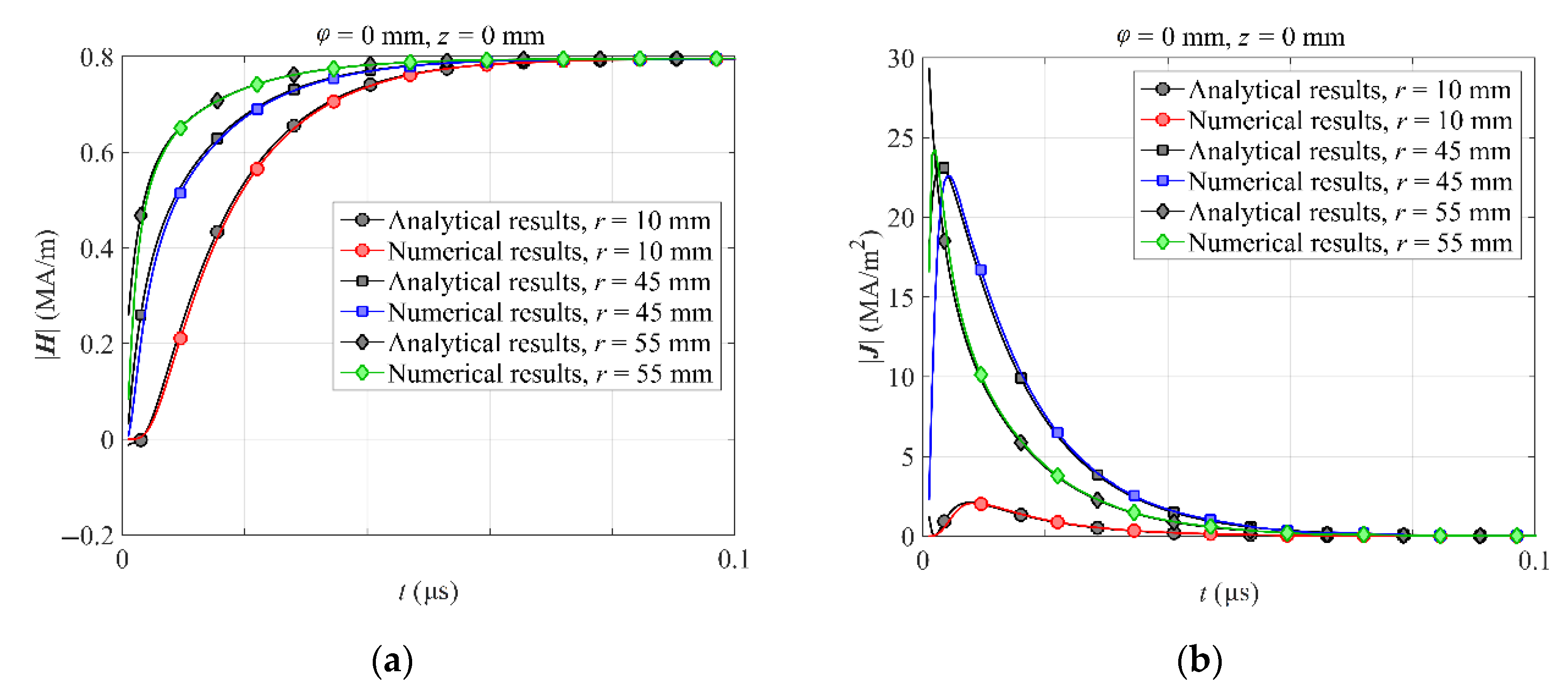
The exemplary calculations were performed for the radii of the inner a, middle b, and outer c parts of the three-layer cylindrical object equal to 30, 50, and 70 mm, respectively. The exemplary electrical conductivities σ_a, σ_b, and σ_c were set to 8, 17, and 10 S/m, respectively and the relative magnetic permeability μ_r = 1 (μ = μ₀μ_r). In the unit step function, the magnetic field H₁ value was set to 7.95 × 10⁵ A/m. The calculated absolute values of the magnetic field intensity H and the induced eddy current density vectors J are shown in Figure 3 on the left and right, respectively.

In the steady state, the magnetic field completely fills the cylinder’s volume and the induced eddy currents disappear. To verify the obtained results, the analytical calculations were also verified by using the numerical modelling software Comsol Multiphysics, which is based on the FEM procedure. We clearly observed that the analytical and numerical results are in good agreement, proving that obtained mathematical expressions are correct. In this section we derived mathematical expressions for the eddy current density vectors in object’s each layer.

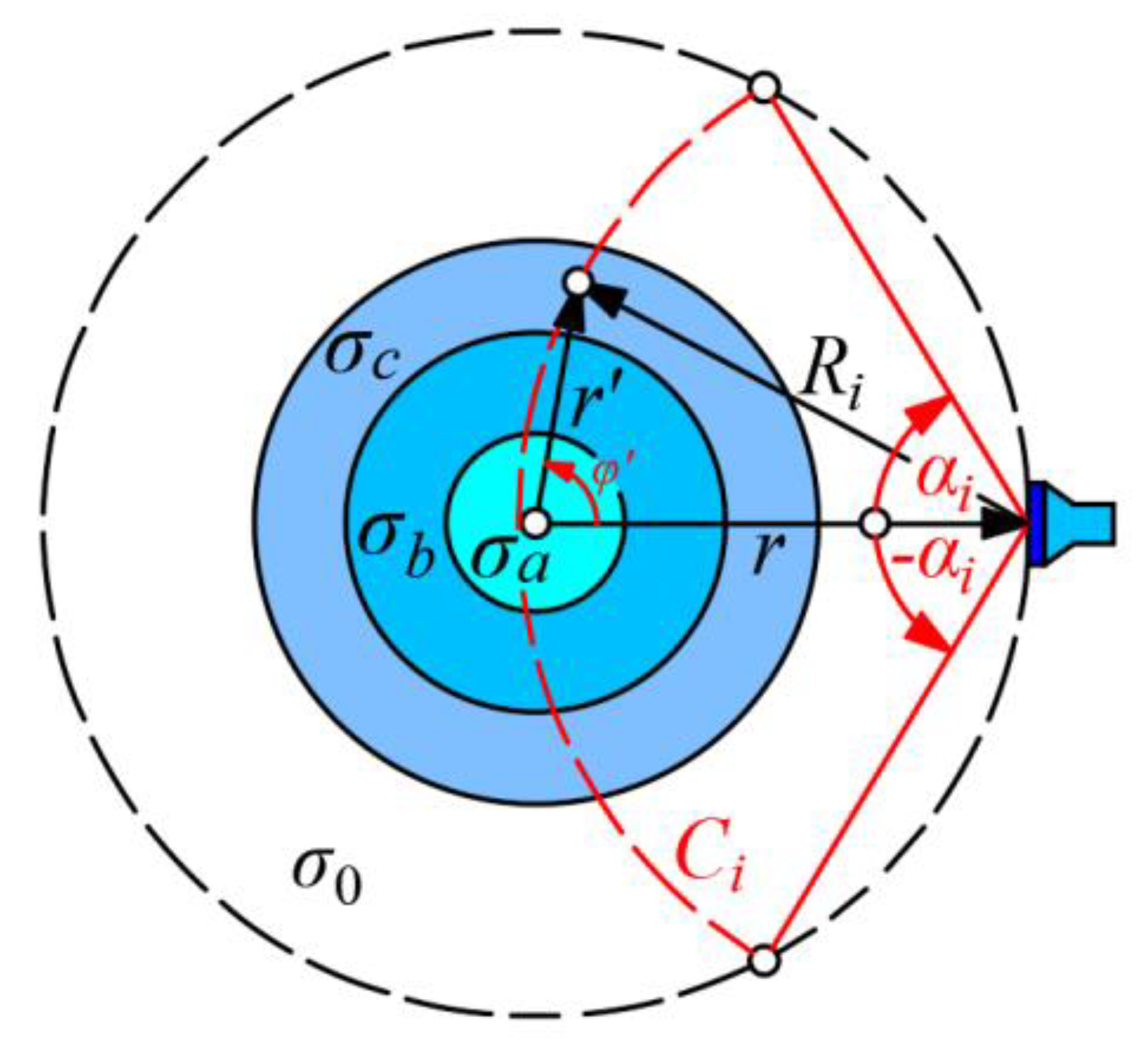
4. Analytical Determination of Acoustic Pressure

Based on Equation (4) and assuming that the induced eddy current density vector J(r’) is bounded in the xy plane, the resultant Lorentz force is expressed as follows [3]:

$$F\left(r^{\prime },{\phi }^{\prime }\right)=F\left(r^{\prime },{\phi }^{\prime }\right)\cdot \cos \left({\phi }^{\prime }\right){\mathbf{1}}_x+F\left(r^{\prime },{\phi }^{\prime }\right)\cdot \sin \left({\phi }^{\prime }\right){\mathbf{1}}_y.$$

(9)

using expression (9), the acoustic pressure at the point of the transducer can be determined by the following formula:

$$\begin{array}{l}p(r,t_i)=\frac{-1}{4\mathsf{\pi }}{\nabla }_r{\displaystyle \underset{C_i}{\int }\mathrm{d}{l}^{\prime }\left[F\left(r^{\prime },{\phi }^{\prime }\right)\cos \left({\phi }^{\prime }\right){\mathbf{1}}_x+F\left(r^{\prime },{\phi }^{\prime }\right)\sin \left({\phi }^{\prime }\right){\mathbf{1}}_x\right]}\frac{1}{R_i}=\\ =\frac{-1}{4\mathsf{\pi }}{\nabla }_r{\displaystyle \underset{-{\alpha }_i}{\overset{{\alpha }_i}{\int }}\mathrm{d}\alpha \left[F\left(r^{\prime },{\phi }^{\prime }\right)\cos \left({\phi }^{\prime }\right){\mathbf{1}}_x+F\left(r^{\prime },{\phi }^{\prime }\right)\sin \left({\phi }^{\prime }\right){\mathbf{1}}_x\right]}=\\ =\frac{-1}{4\mathsf{\pi }}{\nabla }_r\{{\displaystyle \underset{-{\alpha }_i}{\overset{{\alpha }_i}{\int }}F\left(r^{\prime },{\phi }^{\prime }\right)\frac{\left[r-R_i\cos \left(\alpha \right)\right]\mathrm{d}\alpha }{\sqrt{r^2+R_i^2-2r{R}_i\cos \left(\alpha \right)}}{\mathbf{1}}_x}+{\displaystyle \underset{-{\alpha }_i}{\overset{{\alpha }_i}{\int }}F\left(r^{\prime },{\phi }^{\prime }\right)\frac{R_i\sin \left(\alpha \right)\mathrm{d}\alpha }{\sqrt{r^2+R_i^2-2r{R}_i\cos \left(\alpha \right)}}{\mathbf{1}}_y}\}.\end{array}$$

(10)

where α_i and −α_i are the upper and lower limits of integration, respectively (Figure 4), and

$$\begin{array}{l}{R}_i=t_i{c}_s,\begin{array}{cc}& \mathrm{d}{l}^{\prime }=\end{array}{R}_i\mathrm{d}\alpha ,\begin{array}{cc}& {\left(r^{\prime }\right)}^2\end{array}=r^2+R_i^2-2r{R}_i\cos \left(\alpha \right),\\ \begin{array}{cc}& \sin \left({\phi }^{\prime }\right)=\frac{R_i}{r^{\prime }}\sin \left(\alpha \right),\begin{array}{cc}& \cos \left({\phi }^{\prime }\right)=\frac{r-R_i\cos \left(\alpha \right)}{r^{\prime }}.\end{array}\end{array}\end{array}(i = 1, 2, \dots )$$

(11)

Figure 4 shows the conceptual framework of the MAT-MI forward problem for the determination of the acoustic pressure at the transducer location. The ultrasound transducer scans the object around a circle, and both the object and the transducer are immersed in pure water (σ₀ ≈ 0) for better ultrasound coupling. Here, the given layers of the three-layer cylindrical object under consideration represent the adjacent acoustic pressure sources. For each transmission time t_i, the detected pressure was the sum of all the sources on each detection arc C_i with the transmission distance R_i, which can be considered as one analogous source on the normal direction of the ultrasonic probe. For the calculation approach, C_i are arcs on which the integration will be performed, according to (10), to determine the acoustic pressure at the point of the transducer location for each transmission time t_i, in the interval [−α_i, α_i]. The length of the C_i arcs are in the range from 0 (at the point of the transducer location) to $\mathsf{\pi }r/\sqrt{2}$ (where R_i is equal to $\sqrt{2}r$) and back to 0 (R_i is equal to 2r), which corresponds to the consecutive angles 2α_i between 180 and 0 degrees.

In acoustic pressure detection, each transducer has its own characteristics of centre frequency, bandwidth, and sensitivity. The system transfer function h(t) = R(t)⊗[∂B₁(t)/∂t] is defined as the convolution of the impulse response of the piezoelectric transducer, which produces a time-series vibration for the acoustic excitation and the derivative of the pulsed magnetic field concerning time t. Finally, the resultant acoustic signal w(r, t) received by the transducer is a convolution between the collected acoustic pressure p(r, t) and the transfer function h(t) and is expressed as follows [22,27,28,29,30]:

$$w(r,t)=p(r,t)\otimes h(t),$$

(12)

where ⊗ is the convolution operator.

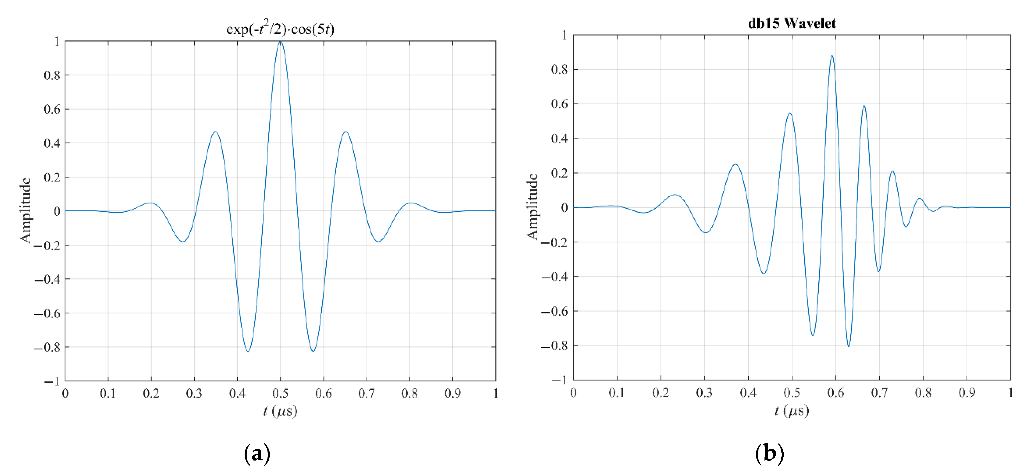
To obtain real shape collected waveforms, it is important to correctly choose the impulse response R(t) shape of the transducer. In MAT-MI measurements such a data is usually provided by the transducer’s manufacturer. However, for our calculations we adopted several mother wavelets which faithfully reproduce the actual shape of the impulse response of typical ultrasonic transducers (e.g., PBP Optel Sp. z o. o.—center frequency of 0.5 MHz, diameter 25 mm, material polyacetal). Among them we chose the Morlet and Daubechies (db15) wavelets, which shapes are shown in Figure 5, on the left and right, respectively. During performing the reconstructing the image with these wavelets we did not notice significant changes in the obtained images’ quality and therefore we decided to use the Morlet wavelet for further calculations.

According to the given formulas and the results of the eddy current distribution obtained in the previous section in the whole volume of the chosen object, the acoustic pressure and corresponding acoustic waveforms at the point of the transducer were computed. For simplicity, the acoustic environment was considered to be acoustically homogenous without any reflections, dispersion, or attenuation, which makes the studies ideal. In calculating the measuring points, transducer equivalents were used. The measuring points were placed on the circumference of the virtual circle with an angle step (scanning step) of 1°. The velocity of sound was set to 1500 m/s for the object and environment. The calculation grid was set to 0.05 mm, and the sampling frequency was set to 100 MHz. 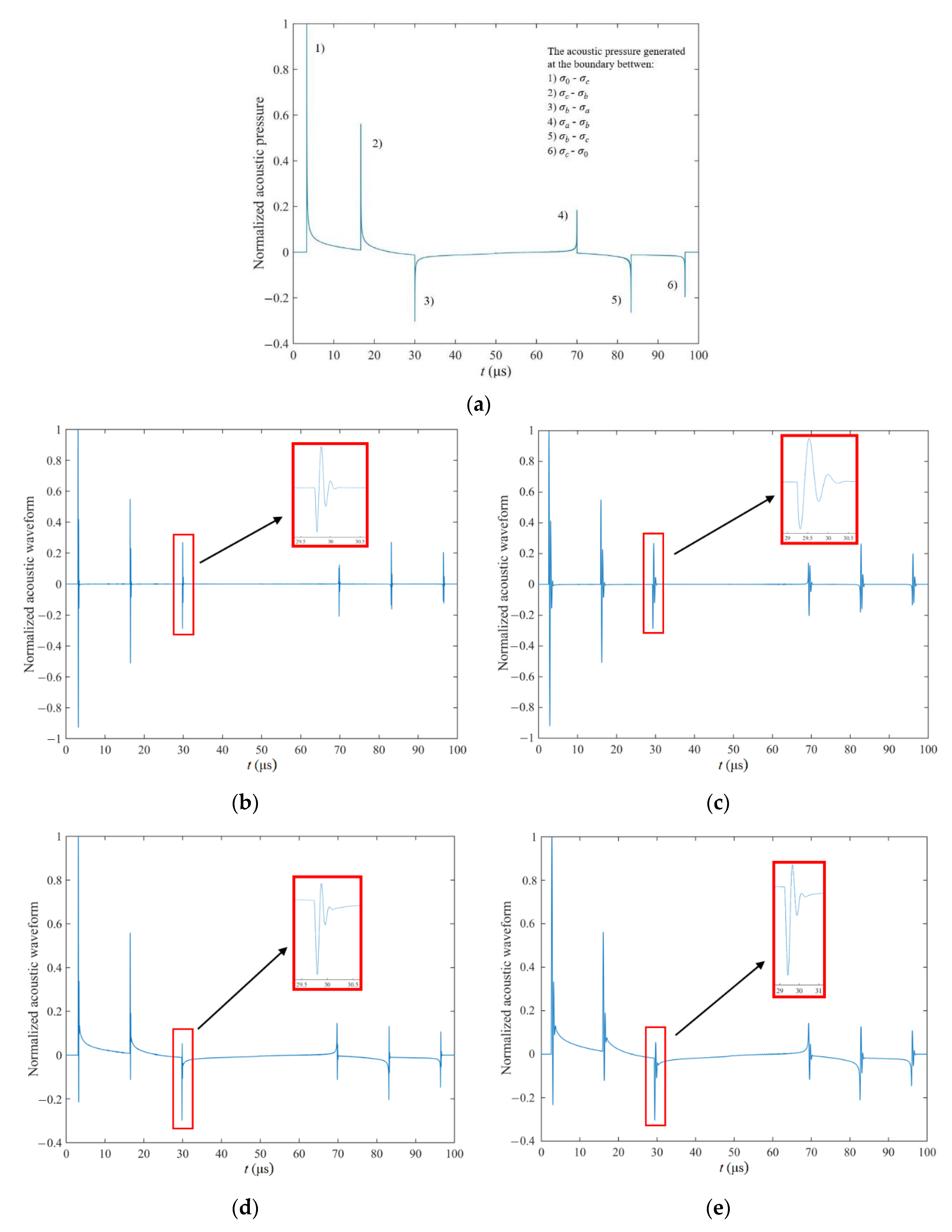As shown in Figure 2b, the distribution of the acoustic pressure determined at (75, 0) mm is presented in Figure 6a, which is normalized by the maximum pressure.

Three positive pressure peaks (at 3.4, 16.7, and 70 μs) and the negative pressure peaks (at 30, 83.4, and 96.7 μs) are distinctly displayed and represent the six object’s boundaries between the three regions with three different conductivities (see Figure 2 and Figure 4). The peaks with positive polarity represent the boundaries where the conductivity change from a lower value to a higher one along the transmission path, while the peaks with negative polarity denote the conductivity’ change from a higher value to a lower one. In addition, although the strengths of the acoustic sources for the whole boundary are the same, the amplitude of the peak at 3.4 μs is higher than that of the peak at 96.7 μs as presented in Figure 6a due to the shorter transmission distance to the transducer (measuring point).

In Figure 6b–e, the acoustic waveforms normalized by their maximum amplitude, obtained after convolution between the calculated acoustic pressure and the system transfer functions shown in Figure 5a,b for two different the centre frequencies are presented. For these figures, the six wave clusters are clearly displayed and correspond to the actual location of the six acoustic pressure peaks illustrated in Figure 6a. The amplitudes and vibration polarities of these wave clusters are generated by the corresponding vertical pressure jumps, reflecting the polarities and values of the conductivity changes between the regions with different conductivities. For example, the two opposite cluster vibration polarities located at 30 and 70 μs with a time interval of 40 μs define the boundaries of the III region (the region with σ_a) of the inner part of the object.

In this section we derived the closed-form analytical formula for the Lorentz force as an interaction of static magnetic field and eddy currents caused in the conductive layers. Additionally, we presented acoustic pressure and acoustic waveforms. In our calculations, the impulse response of the transducer was simulated by the Morlet wavelet.

5. Reconstructing the Acoustic Wave Source

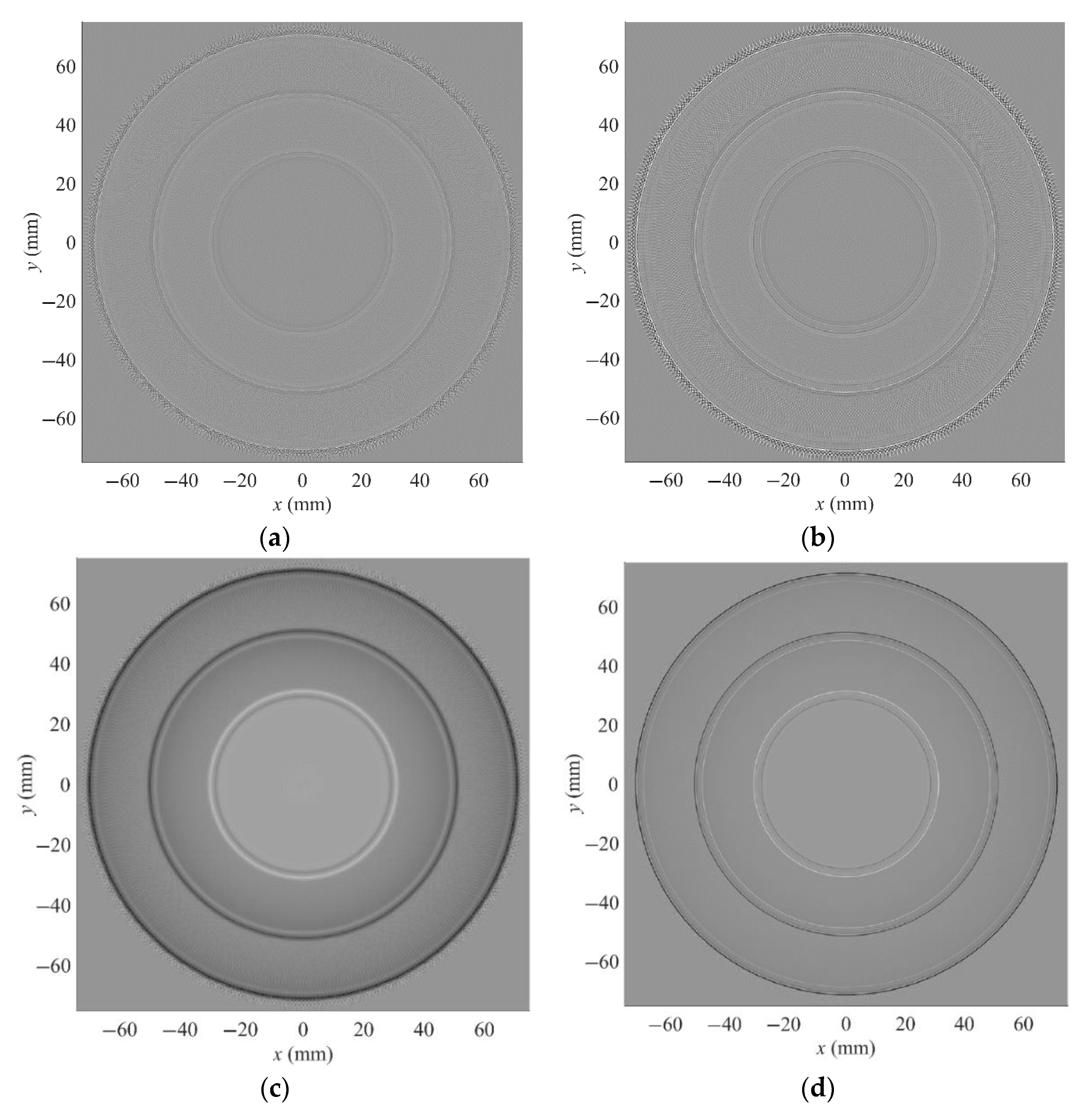
Based on the back-projection algorithm of Equation (5), the acoustic source reconstruction as a Lorentz force divergence distribution of the traditional MAT-MI image was reconstructed as illustrated in Figure 7a–d with the 360 calculated waveforms collected around the object. Three coaxial rings with the radii of 70, 50, and 30 mm are displayed, which are consistent with the cross-sectional conductivity distribution in Figure 2 and Figure 4 in terms of shape and size. The boundary colours of the outer and middle mediums are different than that of the inner medium due to the polarity of the pressure peaks visualized in Figure 6a.

Let us now take a look at the stripes constituting the reconstructed borders between the conducting regions. Two main differences between Figure 7a–d are observable, namely the width and uniformity of the stripes obtained. The stripe at each conductive boundary makes a wide borderline between the adjacent region with a width that is dependent on the centre frequency of the system transfer function that is related to the length or size of the used waveform. The borderlines displayed in Figure 7a,c are wider than the borderlines presented in Figure 7b,d that are compatible with the used centre frequencies of the system transfer functions in the case of 1 and 0.32 MHz, respectively. The outer reconstructed boundaries shown in Figure 7a,b are heterogeneous; there are no stripes with equal values (the stripes are not uniform) as opposed to the boundaries illustrated in Figure 7c,d where the pixels of equal value create circular stripes.

6. Reconstruction Example for Complex Shape

In this section, examples of acoustic source reconstruction for objects of complex shape and complex conductivity distribution are provided. Generally, the source term ∇·(J × B₀) of the ultrasonic wave Equation (3) can be figured out with the time-reversal approach (5). The MAT-MI forward and inverse problem simulations were performed with FEM, using Comsol Multiphysics software.

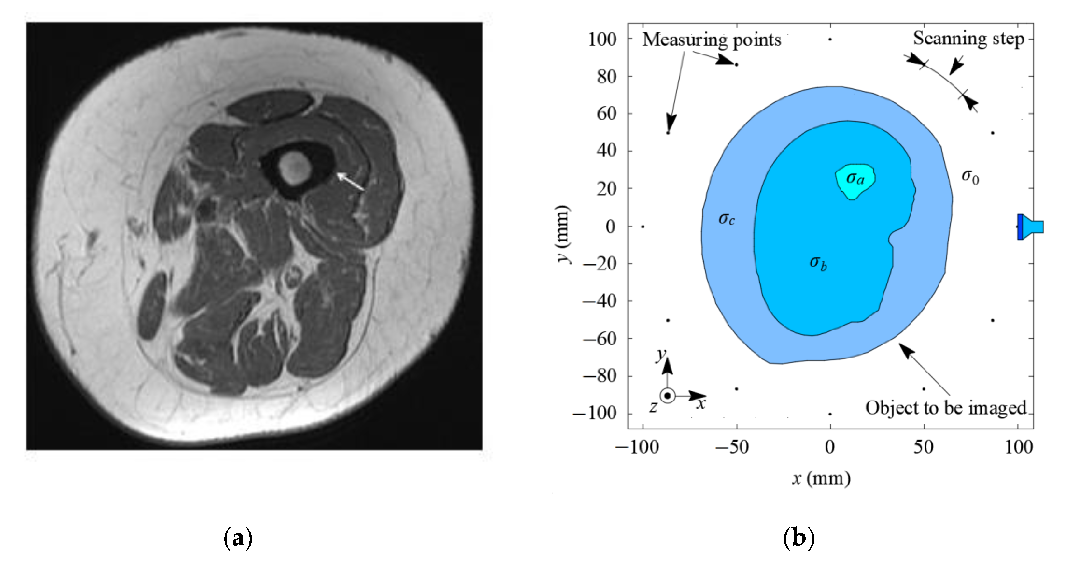
Our idea was to build a MAT-MI model with an object that would resemble a cross-section of the human thigh, containing bone, muscle, and fat. In the case of objects with complex shapes where it is very difficult (in many cases, impossible) to find analytical solutions for the eddy current distribution, a numerical procedure must be applied.

Figure 8b shows the considered 2D planar geometry that was built based on the magnetic resonance imaging (MRI) image of the human thigh presented in the Figure 8a [31]. The three-layer conducting object to be imaged is placed non-concentrically in the non-conductive environment (σ₀ = 0), under the action of two external static and time-varying magnetic fields. In calculations, the amplitude of the static magnetic field with the flux density B₀ was set to 1 T, and, in the unit step function, the pulsed magnetic field with the flux density B₁(t) value was set to 1 T. The electrical conductivities of the inner, middle, and outer layer of the object (equivalents of the human femur, muscle, and fat) were set to σ_a = 5.73 × 10⁻² S/m, σ_b = 4.35 × 10⁻¹ S/m, and σ_c = 3.50 × 10⁻³ S/m, respectively [32]. The relative magnetic permeability value μ_r was set to 1 and this is the same for each object’s layer. We assumed that the layers were acoustically homogeneous without any reflections, dispersion, or attenuation, which indicates that the studies were ideal (recorded signals were considered as a noise-free). The acoustic velocity c_s was set to 1500 m/s. The measuring points (real transducers’ equivalent) were placed on the circumference of the virtual circle with a radius equal to 100 mm. 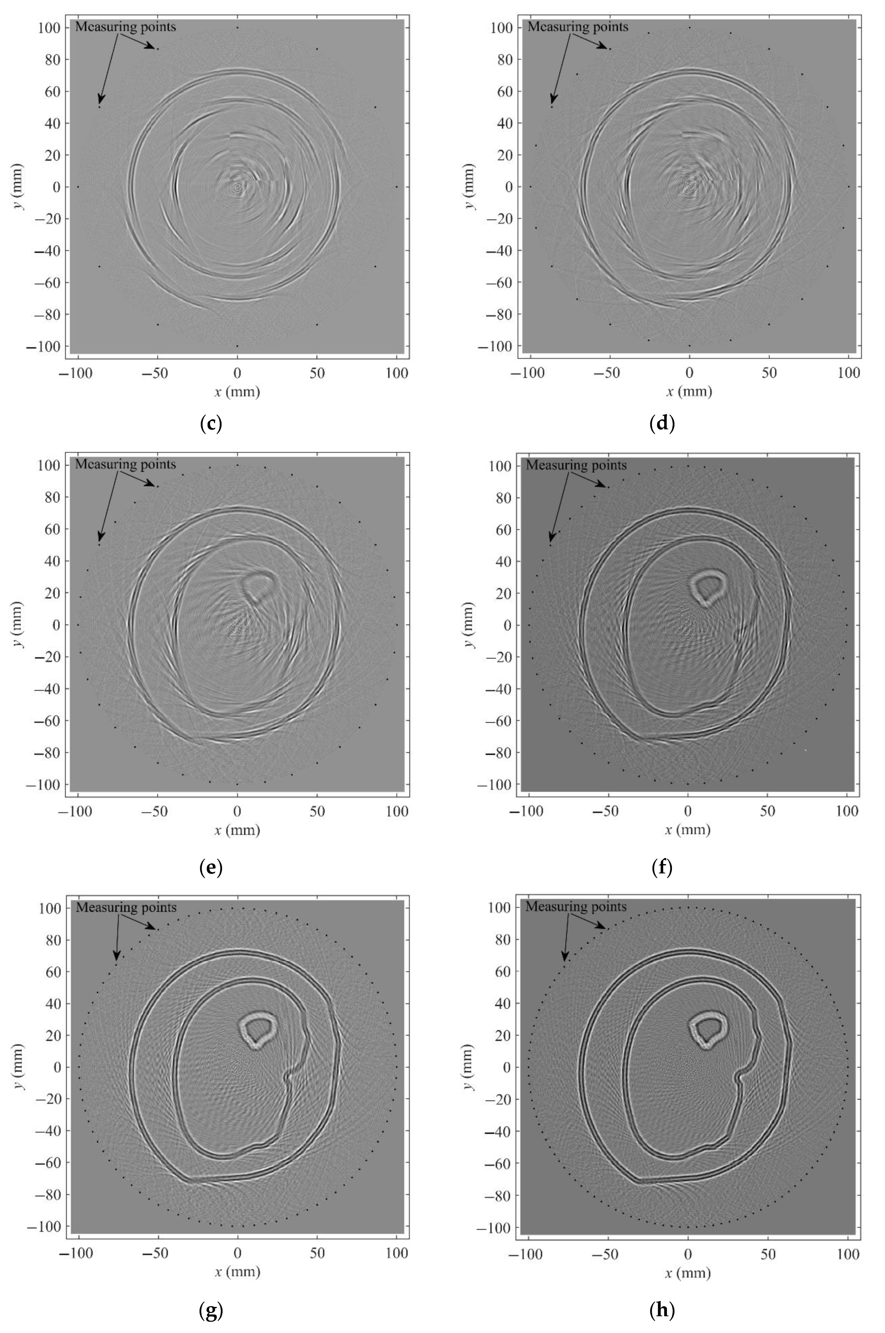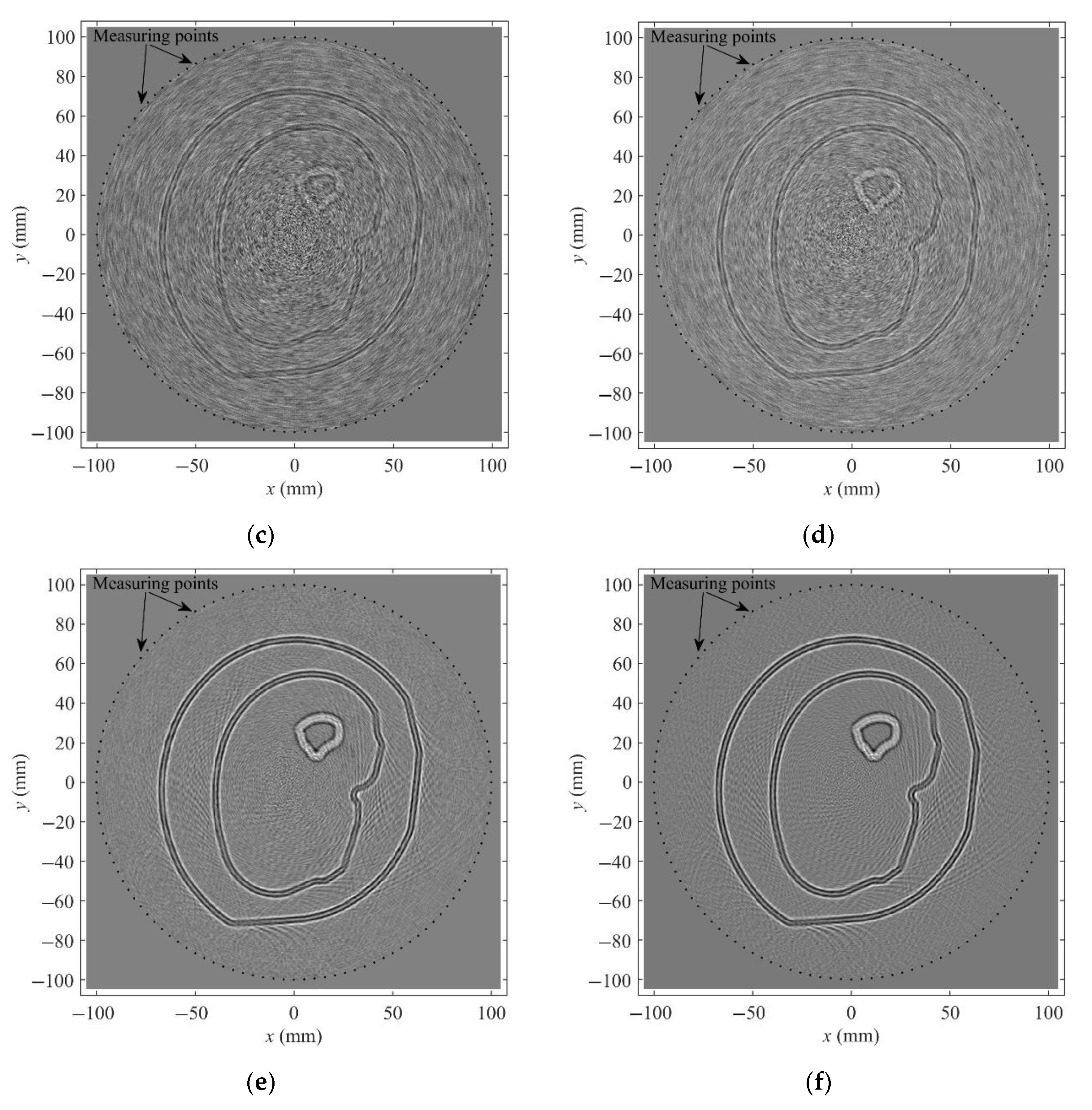In Figure 8c–h, we present the results of the reconstructing the object for different numbers of measuring points.

The subjective assessment is undoubtedly pointing at more measuring points leading to a better-quality image with less time-reversal noise. We observed that, in the case of 12 measuring points (30° scanning step), limited information regarding the layers of the object is revealed (Figure 8c). For 24 measuring points (15° scanning step), some features of the object (boundaries) begin to emerge; however, blurring artifacts inside and outside the object can be observed. With the 6° scanning step (Figure 8f), the reproduced ultrasonic source locations almost perfectly correspond to the real positions of the objects. Significant image reconstruction improvement occurs when the scanning step is around 4° (90 measuring points). Further decrements of the scanning step did not greatly change the image.

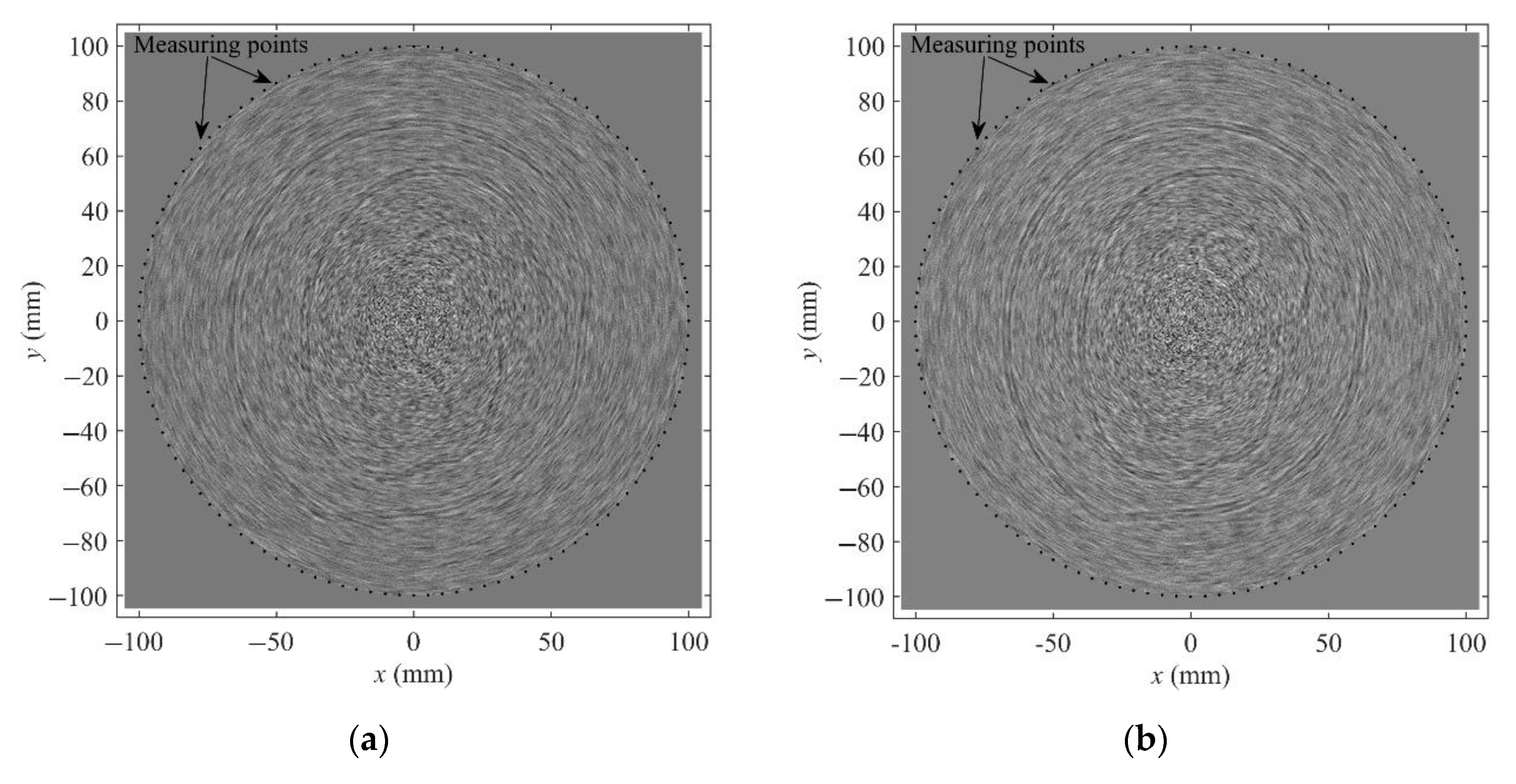
From practical point of view, it is very important to estimate the quality of image reconstruction in the presence of noise of a value typical for the analyzed tomography. A typical value of the signal-to-noise ratio (SNR) of the MAT-MI measurement systems and related tomography methods is the value of 20 dB [21,30,33,34]. Its value depends mainly on a few basic factors, which include: the distance of the transducer from the tested object, the characteristic parameters of the transducer (shape and size). In addition, the SNR of the imaging system is not only determined by the characteristic parameter of the transducer, but also affected by other factors which contain the static magnetic field strength, time-varying magnetic field strength (quality of the excitation), or temperature and type of coupling medium and so on. Another factor influencing the SNR value is the quality of the devices that make up the measurement system. A good quality amplifier can introduce a noise of 40 dB [20]. To examine the influence of noise on the quality of the reconstruction we added to the received signal Gaussian white noise with different SNRs levels: 3 dB, 5 dB, 8 dB, 10 dB and 25 dB, 40 dB, for very noisy and less noisy images, respectively. The figures Figure 9a–f show the results of the image reconstruction for 3° scanning step.

In the restored images, certain blurring artifacts are observed, especially in the case of SNRs level of 3–10 dB, as expected. However, less noise (25–40 dB SNRs level) leads to better quality images. In case of 40 dB SNR the restored ultrasonic source locations almost perfectly match the physical position of the objects. In this case, the general image contrast is properly restored, with some small interference located at the objects’ edges.

In this section we successfully performed the numerical image reconstruction of the three-layer low-conductivity object of complex shape. The influence of scanning resolution and noise values on the quality of the reconstructed image is shown.

7. Conclusions

In this paper, we analysed and compared analytical and numerical models of magnetoacoustic tomography with magnetic induction. According to the first stage of the MAT-MI forward problem, mathematical expressions for the transient magnetic induction effect with Lorentz forces were derived, and the results of the analytical calculations were validated with those obtained from the developed 2D finite element numerical model. For the given formulas and the results of the eddy current and Lorentz force distribution obtained in the whole volume of the chosen objects, the acoustic pressure and corresponding acoustic waveforms at the point of the transducer were calculated. In the case of the MAT-MI inverse problem, the three-layer objects of the simple and complex shapes of the layer boundaries and conductivity distributions were considered. The conditions related to the scanning resolution and noise value, which allow for a successful image reconstruction, are also given.