Abstract
In this paper, an accurate model to simulate the dynamics of the flow of synthetic jets (SJ) in quiescent flow is proposed. Computational modeling is an effective approach to understand the physics involved in these devices, commonly used in active flow control for several reasons. For example, SJ actuators are small; hence, it is difficult to experimentally measure pressure changes within the cavity. Although computational modeling is an advantageous approach, experiments are still the main technique employed in the study of SJs due to the lack of accurate computational models. The same aspect that represents an advantage over other techniques also represents a challenge for the computational simulations, such as capturing the unsteady phenomena, localized compressible effects, and boundary layer formation characteristic of this complex flow. One of the main challenges in the simulation of SJs is related to the fact that the spatial and temporal scales of the actuator and the corresponding flow control application differed in several orders of magnitude. Hence, in this study we focus on the use of Computational Fluid Dynamics (CFD) and Reduced Order Models (ROM) to develop an accurate yet low-cost model to capture the complexities of the flow of a SJ in quiescent flow. Numerical results show two possible paths for SJ modeling; (1) to obtain a boundary condition to predict velocity profile and jet formation from experimental data of diaphragm’s deformation; and, (2) to predict peak velocity at the jet’s outlet with a ROM approach and to use the physical details of the actuator to develop an accurate boundary condition for CFD. Both approaches are validated through experimental data available in the literature; good agreement between results from CFD, Lumped Element Model (LEM), and experimental data are achieved. Finally, it was concluded that the coupling between LEM and CFD is a novel and accurate approach, which improves CFD due to the advantages of LEM closing the gap between LEM’s lack of flow detail and CFD’s lack of geometrical/physical information of the actuator.
1. Introduction
Over the last few decades, flow control has been an important topic in fluid dynamics applications, such as aerodynamics, heat transfer, acoustics, and fluid transport. The main strategies for active flow control are classified in fluidic mechanisms or strategies that alter the shape of the body [1]. Considering external flows, the goals of a control flow technique are mainly transition delay, avoiding or delaying flow separation, lift increasing/drag reduction, and noise suppression, among others [2].
Fluidic actuators, such as Synthetic Jets (SJs), have been proven to be one of the most promising technologies due to the effects produced on the overall flow requiring low input power [3]. A SJ consists of an oscillating diaphragm placed in a cavity driven by electromagnetic, acoustic, mechanical, or piezoelectric actuators. The oscillation of the diaphragm produces an effect of suction and ejection of fluid through an orifice connected to the cavity by a neck. The oscillating blowing and suction produces a stream of vortices shedding upward the orifice to the external flow during the so-called expulsion stage.
To achieve a real impact on the outer flow, the momentum of the actuated flow must be large enough, hence the stream of vortex travels at high velocity; therefore, a high momentum flow is injected into the surface. Using the right amplitude and frequency, the external boundary layer flow can be energized and controlled [4]. The energy transferred by pulsed air directly influences the flow behavior both locally (near the actuator) and globally (in the outer flow) [5,6]. Since the effect of transferring momentum and high energy flow to the surroundings is performed without mass transfer, SJs are often called Zero-Net Mass Flux (ZNMF) devices [7,8].
In quiescent flows, behavior is subject to several parameters, which are related to the actuator’s geometry (e.g., orifice size, orifice shape, and cavity’s shape), operation (e.g., frequency, amplitude), and fluid characteristics (e.g., density, mean velocity, viscosity). Thus, it is common to employ dimensionless parameters to determine an actuator’s response, some of the most well-known are Reynolds Number (Re) and the Stroke Length, which is the column of fluid displaced during the blowing phase [3]. This parameter is related to the Strouhal number (Sr) as it is equal to its inverse; therefore, in many studies, the Stroke Length is employed as a dimensionless frequency rather than a dimensionless amplitude [9]. Jabbal et al. [10] in their experimental study of a round SJ in quiescent flow discussed the role of these dimensionless numbers on the jet’s behavior. It was concluded that an increase of the Stroke Length produces an increase in the streamwise spacing of consecutive vortex structures formed by the jet. Besides, it was also found that an increase in the Reynolds number shows an increase in the vortex ring strength.
By employing dimensionless numbers, Utturkar et al. [11,12] proposed a jet formation criterion (K) that states the necessary condition for a SJ existence. This criterion is defined as the expected value for which a time-averaged outward velocity appears along the jet axis leading to the generation and subsequent convection of a vortex ring. Jet formation is governed by dimensionless parameters, such as Stroke Length (or Strouhal Number), Reynolds Number, and Stokes Number as follows . A typical value of K for two dimensional SJs is 1 and 0.16 for axisymmetric SJs [12].
Jets behavior is highly influenced by geometrical parameters such as, aspect ratio (AR). A slotted jet can affect jet velocity, enhance axis switching phenomena while the AR increases, therefore, increasing jet velocity [13]; AR can affect vortex formation and the jet centerline velocity [14]. Cavity dimensions, such as height, can also affect induced velocity. Mallinson et al. [15] and Mane et al. [16] showed that a larger cavity height yields lower induced velocity while decreasing cavity height would produce the opposite effect. Bazdidi-Therani et al. [17] agree with this observation in their computational study of a SJ flow in compressible regime using dynamic mesh for modeling the diaphragm deformation. Utturkar [18] observed that changes in the cavity aspect ratio have limited effect on the jet exit; concluding that details of cavity design and diaphragm placement do not have an important role in jet performance.
After experimentally study, an array of twelve slotted jets in quiescent flow, Ceglia et al. [19] found that in the spanwise direction the velocity magnitude is uniform at the jet exit; however, downstream, the interaction between SJs causes the external jets to bend towards the inner ones that enhances turbulent dissipation. Many other studies regarding the effects of geometrical parameters on SJs in quiescent flow are discussed by Hong et al. [20], concluding that despite several studies over the last few decades, there is a need of further investigation especially in regard to the AR effect since findings have been contradictory.
SJs behavior has been extensively studied from an experimental and a numerical point of view. However, to carry out an experiment, it is expensive and challenging due to the small geometries involved and the instabilities of the flow. On the other hand, a computational approach allows to not only capture flow details, but also to obtain results for multiple configurations and conditions with lower costs. However, computational simulations are demanding in terms of computational resources, due to the need of capturing details of flow within and without the actuator by modeling the complete three-dimensional geometry of the actuator including diaphragm deformation. Therefore, simplifications of the actuator and the flow within the cavity have been largely employed with good results. In addition, numerical simulations must not only ensure the development of high quality grids especially refined in the cavity, orifice and jet slot; but also to solve compressible flow effects due to low Mach number (Ma) near the diaphragm O(10−3) and high Ma O(101) in the jet’s outlet [3]. Therefore, the advantage that a computational approach presents is sometimes surpassed by experiments with innovative visualization techniques, such as Particle Image Velocimetry (PIV) that provides accurate flow details. To assess Computational Fluid Dynamics (CFD) capabilities that are used to predict jet flow physics, a validation workshop was held in 2004 [21]. Three cases were proposed: slotted SJ in quiescent air, axisymmetric SJ in crossflow and flow over a hump model. In the first case, to avoid fully resolving the cavity’s flow, a velocity profile boundary condition was used. It is worth noting that none of the three-dimensional studies modeled the actual geometry of the actuator. Rather, it was simplified, keeping geometrical parameters, such as cavity aspect ratio and orifice aspect ratio constant. Those who modeled flow inside the cavity set a time dependent velocity boundary condition. CFD capabilities have grown since then, however, and many of those simplifications are still employed today. Table 1 summarizes some of the models typically employed in CFD.

Table 1.
Models for representing synthetic jets in numerical simulations.
The most accurate models of SJ are based on numerical solutions of three-dimensional (3D) Navier–Stokes Equations in the cavity flow and the outer flow. On the other hand, reduced order models are based on assumptions of flow behavior that simplify the problem and allows obtaining accurate results for global variables of interest. Table 2 summarizes some of the reduced order models employed the simulation of synthetic jets.
Table 2.
Reduced Order Models for representing synthetic jets.
For the purpose of designing and optimizing SJs, less complex approaches, such as Reduced Order Models (ROM) that are able to predict the dynamic response of the jet with reasonable accuracy, are employed. Lumped Element Model (LEM) is a well-known ROM that regardless its simplicity provides accurate results. There are two categories to classify LEM [34]. The first is based on an equivalent circuit representation of the elements of the actuator namely, diaphragm, cavity, neck, and orifice [37]; and the second is based on fluid-dynamics equations in which the diaphragm is modeled as a single-degree-of-freedom mechanical system, which is pneumatically coupled to the cavity-orifice [38].
The fundamental idea of LEM is to reduce the complexity of the problem by considering the actuator as a coupled mechanical-acoustic resonator and assuming that variations of flow can be described through discrete components or “lumped” elements connected to each other. The fundamental assumption relies on the physical characteristic length of the actuator that is smaller than the characteristic wavelength of the physical phenomena. This assumption leads to simplify the flow physics decoupling temporal from spatial variations; hence, at each instant inside the cavity, flow depends only on time; therefore, spatial variations are neglected. Then, the governing equations that at first were a set of partial differential equations becomes a set of ordinary differential equations [32,39,40]. Due to the simplicity of LEM and the accuracy of results, this model is a good technique for designing SJs.
Up to now, several issues in the simulation of SJs have been pointed out:
- Geometrical parameters of SJs actuators are important and have a significant effect on the flow behavior that cannot be neglected.
- Capturing flow details is challenging due to small geometries and unsteady behavior, especially within the cavity and jet outlet.
- In order to solve the details of the flow inside the cavity, it is important to understand external flow and its interaction with the flow generated by the SJ. However, it is common practice in numerical simulations to use simplifications to reduce complexities and computational cost.
- Details of the flow inside the cavity would be useful for actuator design purposes and to develop low-dimensional models [24]. When the cavity flow is not solved and the simplifications aforementioned are employed, important parameters such as vorticity or turbulent kinetic energy are unknown.
- Employing a velocity boundary condition imposed on the surface is one of the most used simplifications. Although numerical results are comparable to experimental data or to other simulation models, important flow details remain missing.
- Therefore, there is a need of models that allow us to capture important flow details while simplifying computational simulations.
In this paper, we focus on capturing the jet’s behavior accurately while keeping the geometric parameters simple enough, with the objective of coupling jet response with diaphragm behavior and disregarding the driving source. This is accomplished by first, performing a numerical analysis of a SJ in quiescent flow for both two and three dimensions, simulating flow inside the cavity, and modeling diaphragm deformation by a velocity boundary condition in order to observe flow details and validate the boundary condition in jet formation. Second, LEM is employed to model a SJ with the goal of reaching an agreement between experimental and LEM results. Finally, a new approach that combines the benefits of LEM’s simplicity with the CFD accuracy is presented. Results from the coupling of LEM + CFD are promising, especially regarding accuracy in global parameters, such as peak velocity magnitude.
The main goal of this paper is to propose a framework to simulate SJs while considering design details of the actuator; hence, obtaining accurate numerical results at low computational cost. To accomplish this, this paper is organized as follows. Section 2 presents a numerical analysis of a piezo-electric SJ in two and three-dimensional CFD simulations. The goal of this section is to verify the capabilities and limitations of the numerical simulations when there is no previous detailed design information of the actuator. On the other hand, Section 3 presents another SJ design technique named LEM, which shows good results when predicting global parameters such as peak velocity at the jet’s outlet, but it misses details of fluid dynamics within the cavity and the interaction with the outer flow. Finally, Section 4 seeks to close the gap between the CFD capabilities to resolve flow details and LEM limitations in order to simplify computational simulations while considering the actuator’s design information. Results shows that in most frequencies the coupling CFD + LEM is able to predict accurately the trend of experimental results. However, there is a range of frequencies, especially the frequencies at which the peak velocity occurs, where the magnitude is not well predicted.
2. Computational Fluid Dynamics Simulation
To understand the jet’s behavior in quiescent flow, it is important to capture the formation and the evolution of a SJ to later be implemented as a flow control technique. As has been mentioned, numerical simulation of SJs is a challenging task due to flow physics, mesh quality and appropriate boundary conditions and simplifications. Therefore, two-dimensional and three-dimensional computational analysis in quiescent flow were carried out in order to assess the quality and validity of the implemented model. The actuator selected is an oscillated jet of air ejected through a slot, which is 1.25 mm wide and 33.6 mm long. The slot is placed at the center of the bottom of box of 609.6 mm by 609.6 mm. The alternating flow in and out of the slot is driven by a piezoelectric diaphragm, which measures 50.8 mm in diameter and excited at a frequency of 450 Hz. The flow field experimental database for case 1 in the CFD Validation Workshop (CFDVAL) [41], carried out by Yao et al. [42], consists of measurements obtained by three techniques, PIV, laser Doppler velocimetry (LDV) and hot-wire anemometry; in addition to the flow variables, diaphragm displacement, cavity pressure and cavity temperature were provided. The actuator was flush mounted on an aluminum plate in a glass enclosure; the diaphragm was a piezoelectric mounted on one side of the cavity. Air at standard conditions at sea level in a temperature-controlled room was the working fluid.
2.1. Computational Set-Up
Geometries employed in two and three-dimensional simulations were proposed in CFDVAL [41] workshop with experimental data. For the two-dimensional analysis, the structured grid showed in Figure 1, consists of approximate 200 k quadrilateral elements with refinements in the cavity, near the bottom and jet’s vicinity. The skewness angle of the elements used in the mesh ranged between 0 and 6 degrees; this parameter provides an acceptable level of confidence of the mesh’s quality. This structured mesh was provided by the CFDVAL workshop organizers; hence, it was employed without a convergence analysis.
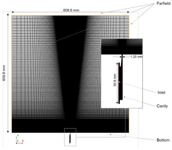
Figure 1.
Computational domain of the two-dimensional quiescent flow case.
The three-dimensional model used an unstructured grid, which is shown in Figure 2 and Figure 3. This grid has a size of approximately 1.3 M tetrahedra elements, and prism elements close to the wall boundaries. Regarding the quality of the mesh, two indicators were used: skewness angle and cell quality. Skewness angle was less than 85 degrees for more than 92% of the total number of cells of the mesh; and more than 80% of the total number of the cells of the mesh have a cell quality close to 1; thus, it was established as a good level of quality for the mesh. The computational domain for the outer flow was defined using the same dimensions of the 2D case, 609.6 × 609.6 × 609.6 mm3, and the cavity represents the exact geometry of the actuator employed in the experiment (see Figure 2).
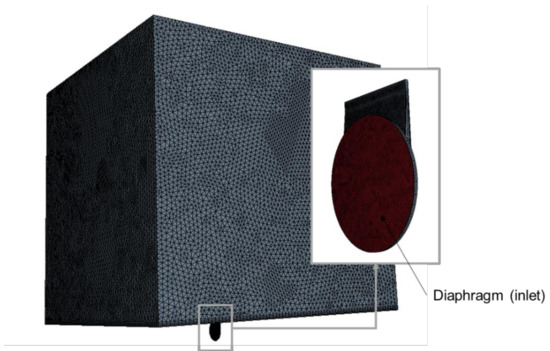
Figure 2.
Computational domain of the three-dimensional quiescent flow case.
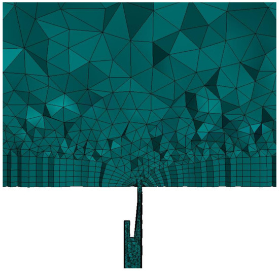
Figure 3.
Close up to the jet’s outlet cross-section volume mesh.
To capture the jet’s formation, the flow inside the cavity was fully solved, unlike in other simulations presented in the validation workshop in which the jet was represented as a normal velocity boundary condition at the synthetic jet outlet. The boundary conditions if the far field were set as an atmospheric constant pressure and slip condition at the bottom of the domain and cavity walls. The synthetic jet is modeled with a velocity boundary condition located at the position of the diaphragm. To model a more realistic diaphragm deformation, it is assumed that it deforms in a parabolic shape, this means that at any time maximum displacement is applied at the center of the diaphragm and decreases parabolically towards the edges that are fixed, Equation (1) shows the profile used along the diaphragm that oscillates in time.
where, is the coordinate along the diaphragm, is the diaphragm diameter, and is the angular frequency of actuation; A is derived from experimental data of the diaphragm deformation. If deformation data are not available, this coefficient should be chosen to match velocity at the jet’s outlet, hence, the jet’s Reynolds number. It is important to note that this boundary condition is derived from experimental data of diaphragm displacement; the velocity proposed implies that diaphragm velocity is equal to fluid velocity.
In the 3D case, a study of sensitivity of the solution to the grid resolution was performed in order to ensure that the numerical results are independent of mesh size. Figure 4 shows the averaged velocity magnitude at the exit of the jet. Five meshes with different total number of cells ranging from to were compared. As it is shown, results for meshes with less than 1.2 M cells are off the asymptotic behavior presented in larger meshes; therefore, in further computations, the mesh with elements was employed. An adequate near-wall cell size was ensured keeping values of y+ not higher than one, especially at the neck and cavity where the time-averaged y+ was below
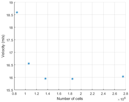
Figure 4.
Mesh independence analysis for the three-dimensional analysis.
The flow solver used in this study was ANSYS Fluent 2020 R2, which employs a finite volume method to discretize and solve the incompressible Reynolds-averaged Navier–Stokes Equations (RANS). Unsteady RANS simulations modeling turbulence with the k-omega SST (Shear Stress Transport) model [43] were performed. This two-equation model has been found to best capture the unsteadiness of the flow due to its accuracy in predicting flow separation and the near-wall behavior that alleviate the shortcoming from other models such as the k-epsilon [44,45,46]. The main advantage of this model in the SJs study is its capability to be employed in both high-Reynolds flows, as well as the near wall region without requiring damping functions for the laminar sublayer [47].
The pressure-velocity coupling was solved with the Semi-Implicit Method for Pressure Linked Equations (SIMPLE). For incompressible and isothermal turbulent flows, this coupling scheme solves the governing equations (mass, momentum, and turbulence) in a segregated manner using a guess-and correct procedure. The mass equation (continuity) is imposed as a restriction rather than being discretized so that a Poisson equation for the pressure is obtained. Once the pressure and velocity fields are known, then the turbulence model transport equations are solved. In unsteady flows, the use of this method, together with the implicit time treatment allowed us to obtain a quasi-steady state of the flow variables with Courant number higher than 1. By using this approach, some instantaneous features of flow might be missing; however, it has been found to be a good approximation of the unsteady flow with accurate results [48]. Time discretization is governed by the frequency of the actuator since it is important to correctly capture the oscillating phenomena, so that the Courant number is not used as a criterion to establish time step. Therefore, simulations were set with a time step of that ensures a correct approximation to the fluid dynamic response up to a frequency of 450Hz. Spatial discretization for pressure, turbulence, and momentum terms were performed with second order schemes. Convergence was set to obtain residuals of O (10−6) with a maximum of 50 iterations per time step. A periodical behavior of the flow was achieved after 10 cycles, and then 25 more cycles were run to obtain unsteady statistics data.
2.2. Numerical Results
To validate the results, both two and three-dimensional cases were compared to experimental data. Figure 5 shows the phase-averaged velocity component along the jet’s direction, which corresponds to the y direction (v-velocity) near the jet outlet. It is shown that there is a phase difference in the expulsion peak between CFD and experiments that is well captured in the suction peak. A similar phenomenon occurs when predicting the time-averaged jet velocity as it is underpredicted in the expulsion phase, but the prediction improves in the suction phase. It is notable that CFD results provide a quasi-symmetric form while the experimental data shows a range of phases where velocity remains constant between expulsion and suction phases. This is explained after the simplifications performed by the model as there are details between diaphragm real deformation and flow behavior that the boundary condition proposed is not capturing.
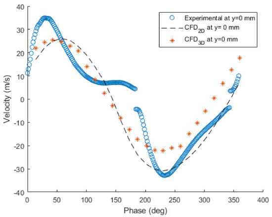
Figure 5.
Comparison v-velocity near jet exit (y = 0 mm), experimental (hot wire anemometer), and Computational Fluid Dynamics (CFD).
For the three-dimensional analysis, velocity along the centerline at the jet’s outlet was plotted against experimental data (see Figure 6). Near the jet’s outlet, the velocity oscillates with a symmetric behavior; however, the farther the jet’s outlet the velocity decays. Although the peak velocity is well captured close to phase 100°, its magnitude is highly underpredicted. This effect is evident in the experimental data and seems to be produced by border effects since it was only captured by three-dimensional analysis. It is noticeable that results from the model employed are independent of grid resolution, only a slight difference is noted 6 mm away from the jet’s outlet. The large difference between numerical and experimental results from y = 3 mm to y = 6 mm is noteworthy. This is attributed to the simplifications posed in the boundary condition. The boundary condition imposed in the diaphragm assumes an almost perfect deformation in parabolic shape, and the suction and blowing phase are symmetric in time, meaning they last the same lapse of time. This behavior is not necessarily accurate since the real behavior of the diaphragm in terms of fluid displacement is unknown. This yields to variations in the strength and convection velocity of the vortex pair that is represented in the peaks of experimental data in Figure 6. In this regard, Zhang and Wang [29] proposed a novel signal wave pattern to generate more efficient SJs. To model the diaphragm deformation a suction/blowing boundary condition is employed, this boundary condition is function of a parameter called “suction duty cycle factor” that affects the cortex strength formed during the blowing phase.
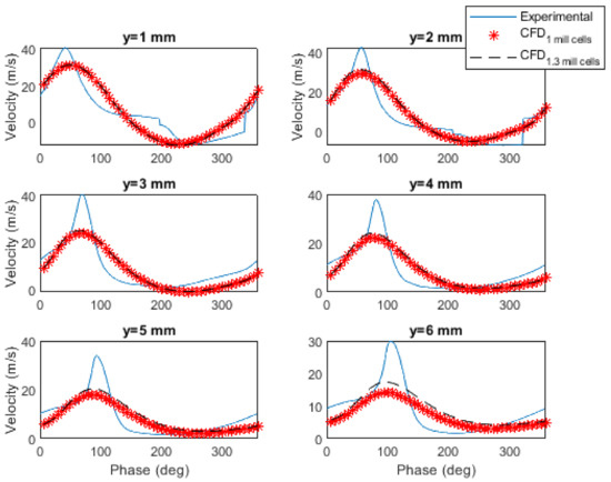
Figure 6.
The v-velocity at centerline jet’s outlet.
Visualization of CFD results of jet’s mean v-velocity across and lengthwise the slot is show in Figure 7. A maximum velocity of 9 m/s is achieved close to the jet’s outlet. Three-dimensional effects are observed in the velocity field along the slot, which cannot be neglected, and it is shown the influence of border effects farther than 10 mm. This aspect validates the accuracy of the SJ model employed in this study since the experiment reports the same phenomena.
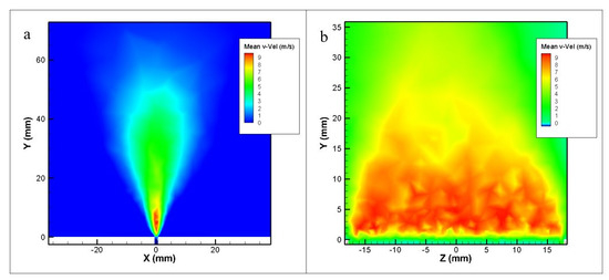
Figure 7.
Time averaged v-velocity across (a) and lengthwise (b) jet’s slot.
Figure 8 shows phase-averaged velocity contours in the vicinity of the SJ outlet. It is clearly observed the jets formation as the fluid is ejected through the slot, after a while jet’s flow experiences an adverse pressure gradient in the region near the orifice, consequently it decelerates the vertical velocity. The instantaneous effect of the pressure is responsible of the synthesized behavior of the jet that is shown in Figure 8.
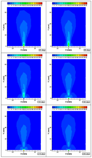
Figure 8.
Phase-averaged velocity magnitude (m/s) in jet formation.
3. Lumped Element Model
The Lumped Element Model (LEM) is a SJ designing technique used to predict the dynamic behavior of electro-mechanic systems. The main assumption is that the characteristic length of the physical phenomena is larger than the characteristic length of the actuator; in other words, the wavelength of the actuator diaphragm oscillation is several orders of magnitude larger than the actuator length La. This assumption is also the main advantage of the model as it decouples spatial and time variations, leading to model flow variations inside the cavity depending on time only. Therefore, reducing the dimensions involved in the problem and resulting in a “lumped” set of Ordinary Differential Equations (ODE’s) governing flow instead of the original Partial Differential Equations (PDE) system.
LEM simplicity implies a major limitation, which is the lack of capturing time-dependent phenomena, for example, modeling the unsteady flow in the orifice and the effects of the injection and ejection phase. Another limitation is that LEM is valid only for compact devices. LEM neglects the pressure spatial variations when where k stands for characteristic frequency and L is the characteristic length; in other words, LEM is valid when the size of the cavity is small compared to the wavelength of the pressure fluctuations [34]. For the same reason, another limitation is that there is a frequency limit beyond which LEM is not valid [3].
To model each part of the actuator by LEM means that some assumptions are made regarding flow behavior. For instance, the orifice/slot model assumes that the flow is fully developed in the neck before it is ejected. This condition is only achieved when the Stroke Length is less than one and limits the model to certain geometrical and operational configurations. However, LEM has proven its value as a predictive and design technique that leads to positive results derived from the dependence of the flow behavior on geometry and materials of the actuator [37].
The electrodynamic actuator selected and analyzed in this section is a double diaphragm and one-hole model consisting of two speakers connected in series. The cavity consists of a support, a vacuum and a lock foils made of acrylic and joined with bolted joints shown in Figure 9; this actuator was experimentally characterized [49].
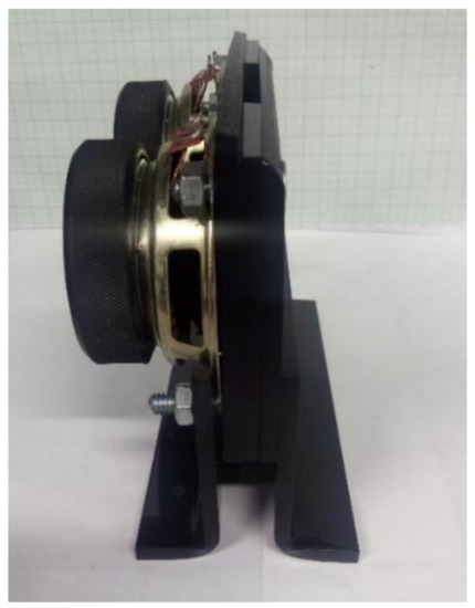
Figure 9.
Electrodynamic actuator double diaphragm.
A SJ involves three energy domains: electric, mechanic, and fluidic/acoustic. The transformation of one domain to another is performed by a two-port model in which effort and flow variables are defined depending the domain of each one. Elements of the actuator, namely, diaphragm, cavity, slot and orifice are represented in an equivalent capacitance circuit [3]. Therefore, the equivalent circuit models the behavior of the actuator according to whether two elements share flow, such as current (i), velocity (U), and volumetric flow (Q), which are connected in series; or whether the elements share effort, such as voltage (V), force (F), and pressure (P), which are connected in parallel.
The equivalent circuit representation of the actuator elements in Figure 10 shows the conversion between the electric domain (purple dashed line) and the fluidic/acoustic domain (yellow dashed line). This conversion is characterized by an electroacoustic transduction coefficient (G) through a two-port model gyrator. Diaphragms (red continuous line) are modeled as a mass-spring-damper system consisting of a resistance, mass or inductance and a capacitance. The SJ cavity (green continuous line) is modeled as an acoustic impedance while the SJ slot (orange continuous lines) is modeled as a resistance and acoustic mass connected in series; both parameters are derived from a two-dimensional analysis of flow in a pipe.
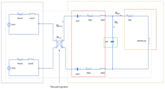
Figure 10.
Equivalent circuit of the double diaphragm electrodynamic actuator.
The transfer function (Equation (2)) that governs the dynamic response of this actuator is derived from the equivalent circuit:
where, , , , . Subindex D represents a parameter of the diaphragm, for example, CaD1 is the acoustic compliance of the diaphragm. Subindex C represents the cavity, for example, CaC is the acoustic compliance of the cavity. Subindex N represents a neck parameter with a linear resistance and mass (RaN, MaN). Ma, rad represents the acoustic radiation resistance and mass of the orifice. G is the electroacoustic transduction coefficient and Q is the volumetric flow rate. For the present study, the main interest is in the volumetric flow rate at the jet’s outlet (Qout).
The results of the model represented by the transfer function (2) are compared to experimental data obtained with a hotwire anemometer for different input voltage [49]. Figure 11 shows agreement between LEM and experimental data for three different induced voltages. A small discrepancy is present as voltage increases show that LEM overpredicted maximum centerline velocity; this is observed close to 100 Hz as the frequency at which the peak velocity occurs is well predicted, but velocity’s magnitude is not, this issue is observed as well by Gallas et al. [34]. However, LEM tends to overestimate experimental data in between two peaks. Luca et al. [50] documented this phenomena, as they find that, for an aluminum shim actuator, LEM overpredicts the experimental results of the average exit flow velocity. The lack of accuracy to predict velocity’s magnitude can be attributed to assumptions and simplifications inherent to LEM.
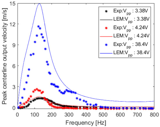
Figure 11.
Peak centerline velocity at jet’s outlet from Lumped Element Model (LEM) and experimental data for different induced voltages.
4. A Proposed Coupling between LEM and CFD
From CFD results in Section 2, it was observed that design parameters of the actuator are important to obtain an accurate solution of the flow. As it was discussed, the different simulations did not account actual diaphragm deformation, rather a relation between diaphragm deformation and flow velocity through frequency of actuation. From the CFD numerical results, it can be concluded that without detailed data of diaphragm deformation, it is difficult to obtain accurate results. Therefore, results could be improved if the boundary condition applied in the diaphragm location accounts for the geometric and physical details of the actuator when experimental data is missing or unknown.
On the other hand, in Section 3, LEM showed a high level of accuracy in results after stablishing an important simplification of the flow inside the cavity, including neglecting pressure variations and assuming fluid fully developed in the neck. Although LEM misses fluid dynamic details due to the inability to capture fluid behavior during the ingestion and ejection phases, peak velocity is well predicted at the frequency that experimental data shows. Nonetheless, velocity magnitude is overestimated and details of the unsteadiness of flow inside the cavity and at the ejection phase are missing.
To exploit LEM’s simplicity and CFD in-deep flow details, a simple coupling of both models is proposed. In this way, the design details that LEM considers serve as input to develop a boundary condition for the CFD simulation, hence, obtaining better results in a simplified manner. It is important to highlight that this methodology has two scenarios in mind that are show in Figure 12. First (Figure 12a), at the stage of SJ design for a specific application (e.g., specific Reynolds Number (Re) or Momentum Coefficient (Cµ) are required), but actuator geometry is unknown, then LEM is employed to design and provide a boundary condition for CFD validation. Second (Figure 12b), if actuator details are known, but flow details are missing (e.g., experiments are out of reach), then LEM is used to provide a boundary condition to study flow behavior through CFD simulations.
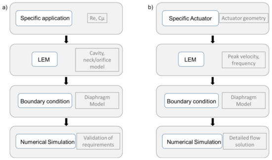
Figure 12.
Methodology proposed to couple LEM and CFD in the suggested cases; (a) Specific application; (b) Specific actuator.
The coupling is achieved after LEM is used to derive the transfer function of the SJ (Section 3), and assuming by continuity that the volumetric flow rate at the orifice’s outlet () must be equal to the volume of flow displaced by the diaphragm per unit of time. Since the boundary condition that is imposed in the CFD model is a velocity inlet/outlet (Dirichlet), then the peak velocity () can be approximated from:
where, is the volume of flow ejected through the orifice, is frequency and is the effective area of the diaphragm. Equation (3) stablishes the relation between the boundary condition used in CFD and the frequency of actuation, this relation is inherent to the design (geometrical and manufacture parameters) of the SJ. Figure 13 shows the diaphragm velocity () for the SJ studied in Section 3 as a function of the frequency of actuation and with an excitation voltage of 3.38 V. For a given voltage and frequency of actuation, is obtained from Equation (3). With , Equation (1) can be implemented as a User Defined Function (UDF) for the boundary condition of the SJ. In the present study, A (peak-to peak amplitude) is equal to , but other possibilities could be implemented, e.g., Root Mean Square (RMS).
Figure 13.
Velocity of diaphragm for an input voltage of 3.38 V.
To test the proposed LEM + CFD method, a CFD model of the SJ studied in Section 3 was implemented. For this, a symmetric 2D computational domain (See Figure 14) in which a diaphragm at the bottom was used. In this case, the geometrical details of the actuator are simplified because it is assumed that this information is captured by LEM. This assumption allows performing a more simplistic computational simulation, since there is no need of having the exact geometry of the SJ. However, the volume of the cavity is the same as in the experiments. A constant pressure boundary condition is imposed in the far field, velocity inlet/outlet is imposed in the diaphragm (as previously explained), and a symmetry condition is used in the jet’s centerline axis. The rest of the boundaries (bottom and cavity in Figure 14) were treated as walls (no-slip). To guarantee the independence of the results, a mesh convergence study was carried out with four different mesh sizes between 300 thousand and 1 million elements. The results showed independence in the value of the flow velocity, just at the exit of the orifice from a mesh of 340 k elements, for this reason, the mesh shown in Figure 14 was used in subsequent simulations.
Figure 14.
Computational domain for the LEM–CFD approach.
From jet simulations in the transient state, the maximum averaged velocity reached in the outlet was obtained according to the inlet condition and for different diaphragm oscillation frequencies (from 50 to 700 Hz). Figure 15 shows the comparison between experimental hot wire anemometer measurements of time-average velocity magnitude at the SJ outlet for an induced voltage of 3.38 V; results from LEM as obtained in Section 3; and results from the CFD + LEM model of time-averaged velocity. It is observed that, for low frequencies, the behavior of the simulations approximates both LEM and experimental behavior; however, it departs from CFD results as the frequency increases. It is noteworthy that the highest velocity is obtained for a frequency close to 100 Hz and it is well captured both by the LEM model and the CFD + LEM results, although the magnitude is not as close to the experimental data due to the documented misprediction effect of LEM that seems to be inherited by the CFD + LEM method.
Figure 15.
Time-averaged velocity magnitude at jet’s exit from coupling LEM and CFD approaches.
The simulation at the highest frequency that was run deviated substantially from LEM results that are better captured at lower frequencies, as it moves closer to the experimental data. This may be due to compressibility effects within the cavity that are not considered in the reduced order model. Additionally, since the fundamental assumption of the model is that the excitation frequency is greater than the characteristic length of the device, it may be that, at high frequencies, this assumption is not correct. It is worth noting that results from CFD + LEM tend to align with experimental data and to separate of LEM’s prediction as frequency increases, this allows us to infer that simulation with CFD + LEM improves LEM’s predictions. Overall, the results from CFD + LEM agree with experimental data, except at the highest velocity; although, the magnitude of the frequency for this condition seems to be well captured. In this regard, refinement of the method should be further investigated.
Figure 16 shows velocity contours of the time averaged v-velocity obtained from numerical computations of the LEM + CFD at a frequency of 300 Hz. Although, there are no experimental data, such as PIV to visualize flow behavior, hence, compare to simulations, it is clearly observed that the jet’s plume is formed as expected.
Figure 16.
Time-averaged v-velocity from coupling LEM and CFD for a synthetic jet (SJ) at 300 Hz.
In order to assess flow behavior and verify the jet’s formation, instantaneous vorticity contours were visualized. During the blowing phase, a street of vortexes is formed upstream; the self-induced velocity of those vortexes should be larger than the mean flow velocity during the suction phase. Therefore, this vortex street cannot be entrained back to the cavity. Following, these vortexes move upstream, farther than the jet’s orifice, leading the formation of a synthetized jet. Figure 17 shows the time sequence of the formation and further upstream propagation of a vortex street, deploying the behavior that is typically expected from SJs. It is clearly observed a sequence of vortexes shedding during the blowing phase. The beginning of vortices formation right at the jet’s exit and its propagation upstream is observed in Figure 17a. Figure 17b shows marked clusters of vorticity with an increasing strength traveling along the jet’s direction. Figure 17c shows the upstream displacement of the vortex previously formed right at the jet’s orifice. Figure 17d shows vortex shedding, and finally, Figure 17e shows the beginning of the suction phase, as the vortex street has completely shed from orifice.
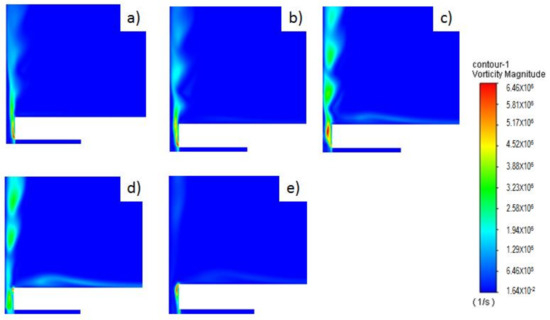
Figure 17.
Sequence of vortex shedding at different phases (θ) for a SJ at 300 Hz. (a) θ = 74°; (b) θ = 78°; (c) θ = 82°; (d) θ = 86°; (e) θ = 90°.
5. Conclusions and Recommendations
Accurate models of SJ for computational simulations are needed specially to assess its flow dynamics for complex engineering applications. The lack of reliable models increases the complexity of simulating the effect of SJ in aerodynamic applications, such as on a wing plane or blade rotors. This is mainly due to the wide range between length and time scales of the actuator and the application. For this reason, details of jet flow behavior are an important aspect in the simulation of SJ applications, but details of the modeling are missing in the state of the art of SJs.
To develop an accurate model to simulate SJs while keeping low computational cost, flow behavior of SJs in quiescent flow was studied. Two paths were discussed, first a computational approach simulating a slotted SJ with an orifice of 1.27 mm driven by a piezoelectric diaphragm excited at 450 Hz. A velocity boundary condition is derived from diaphragm deformation data and employed in a computational simulation of the full actuator including flow behavior within the cavity, neck, outlet, and surroundings. The unsteady RANS simulation with the k-omega SST turbulence model showed the importance of the deformation data for an accurate boundary condition. Additionally, it is noted the importance of three-dimensional computations to capture jet formation and flow behavior since two-dimensional analysis misses important border effects in the formation of the SJ. The implemented model showed good agreement with the experimental data as velocity profile is close to experimental data. However, some details are still missing from the computations; in particular, the peak in the ejection phase is not well captured by the model. In addition, the peak of maximum velocity at different heights along the jet centerline is underpredicted, especially farther from the jet’s outlet. Some refinement to the boundary condition to better resemble diaphragm deformation could be a solution to better predict velocity’s maximum value. Thus, to know physical details of the actuator and, the relation between diaphragm deformation and flow behavior would enhance model prediction.
The second path discussed was to employ reduced-order models as a technique to design SJ and predict its global dynamical behavior for an electromechanically driven actuator. Having the geometrical and physical details of the actuator, a LEM model was developed to predict maximum jet velocity from an induced voltage. Results showed good agreement between experimental and computational results, although the peak velocity for high voltage was slightly underpredicted. It is important to note that, due to the reduced order nature of LEM, instantaneous flow features are missing, but geometrical and physical details of the actuator are captured. Therefore, the coupling between LEM and CFD seeks to close the gap between these two methodologies.
Finally, a novel and simple coupling between CFD and LEM was proposed. The main idea was to develop a LEM model to obtain an expression for volumetric flow rate at the jet’s outlet, and from there, to derive a velocity boundary condition for the simulation. To test this idea, an unsteady RANS computational, and 2D simulation of an actuator of the same cavity volume and orifice size as the studied in Section 3 was performed with the standard k-omega SST turbulence model.
Validation through the peak velocity at the centerline showed good agreement between experiment, LEM, and CFD + LEM method, despite the strong assumptions in the CFD model, especially in the geometry. Qualitative analysis of flow behavior shows the expected jet formation with the vortex shedding phenomena. Regarding the peak velocity comparison, it is possible that at higher frequencies, LEM fails to predict velocity field due to the fundamental assumption that the wavelength of the phenomena is larger than the characteristic length. However, computations with LEM + CFD method showed to follow the experimental trend, leading us to infer that the proposed method improves LEM’s results, and predicts more accurate dynamic response of the actuator. It is possible to conclude that the limitation of LEM’s to capture unsteady features of flow is overcome with the coupling with CFD. Nevertheless, more refinement in this model and further investigations should be done in the range of frequencies the peak of velocity appears, since prediction in that range is not completely accurate.
Author Contributions
Conceptualization, A.M.-C. and O.D.L.M.; methodology, A.M.-C. and O.D.L.M.; software, A.M.-C.; validation, A.M.-C.; formal analysis, A.M.-C. and O.L; investigation, A.M.-C.; writing—original draft preparation, A.M.-C.; writing—review and editing, A.M.-C. and O.D.L.M.; supervision, O.D.L.M. All authors have read and agreed to the published version of the manuscript.
Funding
The APC was funded by the Vice Presidency for Research and Creation publication fund at the Universidad de los Andes.
Acknowledgments
All authors acknowledge financial support for the doctoral student A.M.-C. provided by the School of Engineering and the Mechanical Engineering Department at Universidad de Los Andes. Additionally, the authors acknowledge the contributions of Daniel Velasco, who provided experimental data for the actuator employed in the Lumped Element Model Analysis and the coupling CFD + LEM case.
Conflicts of Interest
The authors declare no conflict of interest.
References
- Doerffer, P.; Barakos, G.N.; Luczak, M. Recent Progress in Flow Control for Practical Flows; Springer International Publishing: Cham, Switzerland, 2017. [Google Scholar]
- Gad-El-Hak, M.; Pollard, A.; Bonnet, J.-P. Flow Control, Fundamentals and Practices; Springer: Berlin/Heidelberg, Germany, 2013. [Google Scholar]
- Mohseni, K.; Mittal, R. Synthetic Jets, Fundamentals and Applications; CRC Press: Boca Raton, FL, USA, 2015. [Google Scholar]
- Montazer, E.; Mirzaei, M.; Salami, E.; Ward, T.A.; Romli, F.I.; Kazi, S.N. Optimization of a synthetic jet actuator for flow control around an airfoil. IOP Conf. Series Mater. Sci. Eng. 2016, 152, 012023. [Google Scholar] [CrossRef]
- Brzozowski, D.P.; Woo, G.T.K.; Culp, J.R.; Glezer, A. Transient Separation Control Using Pulse-Combustion Actuation. AIAA J. 2010, 48, 2482–2490. [Google Scholar] [CrossRef]
- Woo, G.T.K.; Glezer, A. Controlled transitory stall on a pitching airfoil using pulsed actuation. Exp. Fluids 2013, 54. [Google Scholar] [CrossRef]
- Gad-El-Hak, M. Modern Developments in Flow Control. Appl. Mech. Rev. 1996, 49, 365–379. [Google Scholar] [CrossRef]
- Glezer, A.; Amitay, M.; Honohan, A.M. Aspects of Low- and High-Frequency Actuation for Aerodynamic Flow Control. AIAA J. 2005, 43, 1501–1511. [Google Scholar] [CrossRef]
- Hatami, M.; Bazdidi-Tehrani, F.; Abouata, A.; Mohammadi-Ahmar, A. Investigation of geometry and dimensionless parameters effects on the flow field and heat transfer of impingement synthetic jets. Int. J. Therm. Sci. 2018, 127, 41–52. [Google Scholar] [CrossRef]
- Jabbal, M.; Wu, J.; Zhong, S. The performance of round synthetic jets in quiescent flow. Aeronaut. J. 2006, 110, 385–393. [Google Scholar] [CrossRef]
- Utturkar, Y.; Holman, R.; Mittal, R.; Carroll, B.; Sheplak, M.; Cattafesta, L. A Jet Formation Criterion for Synthetic Jet Actuators. In Proceedings of the 41st Aerospace Sciences Meeting and Exhibit, Reno, NV, USA, 6–9 January 2003. [Google Scholar] [CrossRef]
- Holman, R.; Utturkar, Y.; Mittal, R.; Smith, B.L.; Cattafesta, L. Formation Criterion for Synthetic Jets. AIAA J. 2005, 43, 2110–2116. [Google Scholar] [CrossRef]
- Van Buren, T.; Whalen, E.; Amitay, M. Vortex formation of a finite-span synthetic jet: Effect of rectangular orifice geometry. J. Fluid Mech. 2014, 745, 180–207. [Google Scholar] [CrossRef]
- Garcillan, L.; Zhong, S.; Pokusevski, Z.; Wood, N. A PIV Study of Synthetic Jets with Different Orifice Shape and Orientation. In Proceedings of the 2nd AIAA Flow Control Conference, Portland, OR, USA, 28 June–1 July 2004; pp. 1–13. [Google Scholar] [CrossRef]
- Mallinson, S.; Hong, G.; Reizes, J. Some characteristics of synthetic jets. In Proceedings of the 30th Fluid Dynamics Conference, Norfolk, VA, USA, 28 June–1 July 1999. [Google Scholar] [CrossRef]
- Mane, P.; Mossi, K.; Rostami, A.; Bryant, R.; Castro, N. Piezoelectric Actuators as Synthetic Jets: Cavity Dimension Effects. J. Intell. Mater. Syst. Struct. 2007, 18, 1175–1190. [Google Scholar] [CrossRef]
- Bazdidi-Tehrani, F.; Abouata, A.; Hatami, M.; Bohlooli, N. Investigation of effects of compressibility, geometric and flow parameters on the simulation of a synthetic jet behaviour. Aeronaut. J. 2016, 120, 521–546. [Google Scholar] [CrossRef]
- Utturkar, Y.; Mittal, R.; Rampunggoon, P.; Cattafesta, L. Sensitivity of synthetic jets to the design of the jet cavity. In Proceedings of the 40th AIAA Aerospace Sciences Meeting & Exhibit, Reno, NV, USA, 14–17 January 2002. [Google Scholar] [CrossRef]
- Ceglia, G.; Invigorito, M.; Chiatto, M.; Greco, C.S.; Cardone, G.; De Luca, L. Flow characterization of an array of finite-span synthetic jets in quiescent ambient. Exp. Therm. Fluid Sci. 2020, 119, 110208. [Google Scholar] [CrossRef]
- Hong, M.H.; Cheng, S.Y.; Zhong, S. Effect of geometric parameters on synthetic jet: A review. Phys. Fluids 2020, 32, 031301. [Google Scholar] [CrossRef]
- Rumsey, C.L.; Gatski, T.B.; Sellers, W.L.; Vatsa, V.N.; Viken, S.A. Summary of the 2004 CFD Validation Workshop on Synthetic Jets and Turbulent Separation Control. In Proceedings of the 2nd AIAA Flow Control Conference, Portland, OR, USA, 28 June–1 July 2004. [Google Scholar] [CrossRef]
- Xia, H.; Qin, N. Dynamic Grid and Unsteady Boundary Conditions for Synthetic Jets Flow. In Proceedings of the 43rd AIAA Aerospace Sciences Meeting and Exhibit, Reno, NV, USA, 10–13 January 2005; pp. 4047–4055. [Google Scholar] [CrossRef]
- Rizzetta, D.P.; Visbal, M.R.; Stanek, M.J. Numerical investigation of synthetic jet flowfields. AIAA J. 1999, 37, 919–927. [Google Scholar] [CrossRef]
- Kotapati, R.B.; Mittal, R.; Catafesta, L.N. Numerical study of a transitional synthetic jet in quiescent external flow. J. Fluid Mech. 2007, 581, 287–321. [Google Scholar] [CrossRef]
- Moshfeghi, M.; Shams, S.; Hur, N. Aerodynamic performance enhancement analysis of horizontal axis wind turbines using a passive flow control method via split blade. J. Wind Eng. Ind. Aerodyn. 2017, 167, 148–159. [Google Scholar] [CrossRef]
- Zhang, W.; Samtaney, R. A direct numerical simulation investigation of the synthetic jet frequency effects on separation control of low-Re flow past an airfoil. Phys. Fluids 2015, 27, 055101. [Google Scholar] [CrossRef]
- Vatsa, V.N.; Turkel, E. Simulation of Synthetic Jets Using Unsteady Reynolds-Averaged Navier-Stokes Equations. AIAA J. 2006, 44, 217–224. [Google Scholar] [CrossRef]
- Carpy, S.; Manceau, R. Turbulence modelling of statistically periodic flows: Synthetic jet into quiescent air. Int. J. Heat Fluid Flow 2006, 27, 756–767. [Google Scholar] [CrossRef]
- Zhang, P.F.; Wang, J.J. Novel Signal Wave Pattern for Efficient Synthetic Jet Generation. AIAA J. 2007, 45, 1058–1065. [Google Scholar] [CrossRef]
- Xia, H.; Qin, N. DES Applied to an Isolated Synthetic Jet Flow. In Advances in Hybrid RANS-LES Modelling. Notes on Numerical Fluid Mechanics and Multidisciplinary Design; Peng, S.H., Haase, W., Eds.; Springer: Berlin/Heidelberg, Germany, 2008; Volume 97, pp. 252–260. [Google Scholar] [CrossRef]
- Lee, C.Y.; Goldstein, D.B. Two-Dimensional Synthetic Jet Simulation. AIAA J. 2002, 40, 510–516. [Google Scholar] [CrossRef]
- Tang, H.; Zhong, S.; Jabbal, M.; Garcillan, L.; Guo, F.; Wood, N.; Warsop, C. Towards the Design of Synthetic-jet Actuators for Full-scale Flight Conditions: Part 2: Low-dimensional Performance Prediction Models and Actuator Design Method. Flow Turbul. Combust. 2007, 78, 309–329. [Google Scholar] [CrossRef]
- Yamaleev, N.K.; Carpenter, M.H.; Ferguson, F. Reduced-Order Model for Efficient Simulation of Synthetic Jet Actuators. AIAA J. 2005, 43, 357–369. [Google Scholar] [CrossRef]
- Gallas, Q.; Sheplak, M.; Kaysap, A.; Carroll, B.; Nishida, T.; Cattafesta, L.; Mathew, J.; Holman, R. Lumped element modeling of piezoelectric-driven synthetic jet actuators. AIAA J. 2002, 41, 240–247. [Google Scholar] [CrossRef]
- Persoons, T.; Cressall, R.; Alimohammadi, S. Validating a Reduced-Order Model for Synthetic Jet Actuators Using CFD and Experimental Data. Actuators 2018, 7, 67. [Google Scholar] [CrossRef]
- Yamaleev, N.K.; Carpenter, M.H. A Quasi-1-D Model for Arbitrary 3-D Synthetic Jet Actuators. In Proceedings of the 43rd AIAA Aerospace Sciences Meeting and Exhibit, Reno, NV, USA, 10–13 January 2005; pp. 2863–2874. [Google Scholar] [CrossRef]
- Chiatto, M.; Capuano, F.; Coppola, G.; De Luca, L. LEM Characterization of Synthetic Jet Actuators Driven by Piezoelectric Element: A Review. Sensors 2017, 17, 1216. [Google Scholar] [CrossRef]
- Sharma, R.N. Fluid Dynamics-Based Analytical Model for Synthetic Jet Actuation. AIAA J. 2007, 45, 1841–1847. [Google Scholar] [CrossRef]
- Boukenkoul, M.A.; Li, F.C.; Aounallah, M.; Mishra, A.; Dutta, A.K. A 2D Simulation of the Flow Separation Control over a NACA0015 Airfoil Using a Synthetic Jet Actuator. J. Phys. Conf. Ser. 2017, 187. [Google Scholar] [CrossRef]
- Oyarzun, M.A.; Cattafesta, L. Design and optimization of piezoceramic zero-net mass-flux actuators. In Proceedings of the 5th Flow Control Conference, Chicago, IL, USA, 28 June–1 July 2010; pp. 1–26. [Google Scholar]
- Rumsey, C.L. CFD Validation of Synthetic Jets and Turbulent Separation Control. 2004. Available online: https://cfdval2004.larc.nasa.gov/case1.html (accessed on 10 October 2019).
- Yao, C.; Chen, F.-J.; Harris, J.; Neuhart, D. Synthetic Jet Flow Field Database for CFD Validation. In Proceedings of the 2nd AIAA Flow Control Conference Portland, OR, USA, 28 June–1 July 2004; pp. 1–11. [Google Scholar] [CrossRef][Green Version]
- Menter, F.R. Two-equation eddy-viscosity turbulence models for engineering applications. AIAA J. 1994, 32, 1598–1605. [Google Scholar] [CrossRef]
- Adya, S.; Han, D.; Hosder, S. Uncertainty Quantification Integrated to the CFD Modeling of Synthetic Jet Actuators. In Proceedings of the 5th Flow Control Conference, Chicago, IL, USA, 28 June–1 July 2010. [Google Scholar] [CrossRef]
- Baghaei, M.; Bergada, J.M. Analysis of the Forces Driving the Oscillations in 3D Fluidic Oscillators. Energies 2019, 12, 4720. [Google Scholar] [CrossRef]
- Alimohammadi, S.; Fanning, E.; Persoons, T.; Murray, D.B. Characterization of flow vectoring phenomenon in adjacent synthetic jets using CFD and PIV. Comput. Fluids 2016, 140, 232–246. [Google Scholar] [CrossRef]
- Laouedj, S.; Azzi, A.; Benazza, A. New Analysis in 3D-Synthetic Jets Within Numerical Investigation Using CFD Validation Code: Moving Boundary Techniques. Energy Procedia 2012, 19, 226–238. [Google Scholar] [CrossRef][Green Version]
- Tadjfar, M.; Asgari, E. The Role of Frequency and Phase Difference between the Flow and the Actuation Signal of a Tangential Synthetic Jet on Dynamic Stall Flow Control. J. Fluids Eng. 2018, 140, 111203. [Google Scholar] [CrossRef]
- Velasco, D. Control de flujo activo con chorros sintéticos en un cuerpo de Ahmed. Master’s Thesis, Universidad de los Andes, Bogotá, Columbia, 2019. [Google Scholar]
- De Luca, L.; Girfoglio, M.; Chiatto, M.; Coppola, G. Scaling properties of resonant cavities driven by piezo-electric actuators. Sensors Actuators A Phys. 2016, 247, 465–474. [Google Scholar] [CrossRef]
Publisher’s Note: MDPI stays neutral with regard to jurisdictional claims in published maps and institutional affiliations. |
© 2020 by the authors. Licensee MDPI, Basel, Switzerland. This article is an open access article distributed under the terms and conditions of the Creative Commons Attribution (CC BY) license (http://creativecommons.org/licenses/by/4.0/).