Drought Detection over Papua New Guinea Using Satellite-Derived Products

Abstract

This study evaluates the World Meteorological Organization’s (WMO) Space-based Weather and Climate Extremes Monitoring (SWCEM) Demonstration Project precipitation products over Papua New Guinea (PNG). The products evaluated were based on remotely-sensed precipitation, vegetation health, soil moisture, and outgoing longwave radiation (OLR) data. The satellite precipitation estimates of the Climate Prediction Center/National Oceanic and Atmospheric Administration’s (CPC/NOAA) morphing technique (CMORPH) and Japan Aerospace Exploration Agency’s (JAXA) Global Satellite Mapping of Precipitation (GSMaP) were assessed on a monthly timescale over an 18-year period from 2001 to 2018. Station data along with the ERA5 reanalysis were used as the reference datasets for assessment purposes. In addition, a case study was performed to investigate how well the SWCEM precipitation products characterised drought in PNG associated with the 2015–2016 El Niño. Overall statistics from the validation study suggest that although there remains significant variability between satellite and ERA5 rainfall data in remote areas, this difference is much less at locations where rain gauges exist. The case study illustrated that the Vegetation Health Index (VHI), OLR anomaly and the Standardized Precipitation Index (SPI) were able to reliably capture the spatial and temporal aspects of the severe 2015–2016 El Niño-induced drought in PNG. Of the three, VHI appeared to be the most effective, in part due to its reduced incidence of false alarms. This study is novel as modern-day satellite-derived products have not been evaluated over PNG before. A focus on their value in monitoring drought can bring great value in mitigating the impact of future droughts. It is concluded that these satellite-derived precipitation products could be recommended for operational use for drought detection and monitoring in PNG, and that even a modest increase in ground-based observations will increase the accuracy of satellite-derived observations remotely.

1. Introduction

Droughts frequently occur in Asia-Pacific countries affecting many people and impacting on the well-being and economy of populations. Over the past 30 years, droughts have affected millions of people in the western Pacific with the most severe drought events having occurred during El Niño years [1]. Similarly, droughts related to the El Niño–Southern Oscillation (ENSO) are a recurring climate phenomenon in the Pacific Island Countries [2]. El Niño refers to the warm phase of ENSO where there is a warming of sea surface temperatures in the central and eastern equatorial Pacific Ocean. This is typically associated with higher pressure and lower rainfall over mainland Papua New Guinea (PNG) [3]. Impacts of droughts on Pacific islands can be very extreme. For example, in 2011, the Pacific country of Tuvalu experienced severe ENSO-induced drought which resulted in a major water availability crisis [4]. In 2015–2016, PNG was affected by severe drought due to a strong El Niño. PNG is a country in the South Pacific with a population of almost 7 million people, of which 85% rely on subsistence agriculture [5]. The Government of PNG estimated that during the 2015–2016 drought, approximately 480,000 people faced critical food shortages due to subsistence crops failing and extreme water shortages [6].

Impacts of recent severe droughts on Asia-Pacific countries emphasised their vulnerability to prolonged periods of rainfall deficit and highlighted the urgency for improved drought adaptation and mitigation measures. It is expected that climate change will exacerbate drought impact on agricultural yields and the productivity of other economic sectors, further reducing the well-being of populations affected [7]. To assist vulnerable countries with climate change adaptation, especially least developed countries (LDCs) and small island developing states (SIDS), the Climate Risk and Early Warning Systems (CREWS) international initiative was established with the World Meteorological Organization (WMO) as one of the key implementing agencies. In PNG, the CREWS initiative aims to improve the existing drought monitoring network and provide early warnings of drought for the agriculture, water, energy, and emergency service sectors [5].

Accurate monitoring of rainfall is vital for detecting the emergence of drought, assisting governments and communities at risk with decision making, and improving preparedness to reduce its potential impact [5]. Conventional meteorological observations using surface-based rain gauges allow a direct measurement of precipitation, but in many LDCs and SIDS including PNG, rain-gauge networks are sparse and do not provide good spatial coverage. As of 2019, in PNG, a country with an area of about 452,860 km², the official rain gauge network consisted of only 13 weather and climate stations and 7 rain gauge stations [5]. Rainfall over PNG is highly variable and such a limited network is not able to provide an accurate assessment of the spatial distribution of rainfall for such a large country with significant topography.

Rain gauges are also subject to additional biases such as those resulting from poor maintenance and observation procedures [8]. Given that a gauge only measures precipitation at a single location, point observation data may misrepresent precipitation over the broader area due to local effects. For example, the topography of PNG is amongst the most rugged in the world, with altitudes of over 4000 m, and wind-induced effects can result in significant spatial variability in precipitation, especially around mountainous terrain [9].

An alternative approach for drought monitoring is to use satellite precipitation estimates; the spatial coverage and uniformity of space-based observations make them a valuable means for estimating rainfall. Meteorological satellites were first used for rainfall monitoring in the 1970s, providing coverage across most of the globe [10]. The first satellite precipitation estimates were based on recording visible or infrared (IR) radiation, estimating cloud-top reflectivity or temperature from the observed radiation data, and then subsequently linking this to rain rates through empirical relationships [10]. A more direct quantification of rain rates was later developed by using passive microwave (PMW) observations that detect the scattering and emission of radiation from hydrometeors [10]. The drawback is that PMW estimates are hindered by the reduced spatial coverage of PMW space-based instruments compared to their IR counterparts [11].

To capitalise on strengths of both satellite techniques, methodologies to combine the broad spatial coverage of IR precipitation estimates with the increased accuracy of PMW precipitation estimates have been developed. For example, one technique uses IR space-based observations to compute cloud-motion vectors which are then used to advect PMW-derived estimates, allowing precipitation estimates to be made for areas that were not directly covered by PMW satellite passes [11]. The National Oceanic and Atmospheric Administration (NOAA) was the first to develop this methodology, utilising it in their Climate Prediction Center (CPC) morphing technique (CMORPH) precipitation estimation products [11]. The Japan Aerospace Exploration Agency (JAXA) later developed their own version, Global Satellite Mapping of Precipitation (GSMaP) [12].

The potential of satellite precipitation estimates was recognised by the WMO. In 2017, WMO initiated the Space-based Weather and Climate Extremes Monitoring (SWCEM) Demonstration Project to assist countries in the Asia-Pacific region with operational utilisation of satellite precipitation estimates, with a particular focus on monitoring precipitation extremes—accumulated heavy rainfall and drought [8]. The SWCEM products include satellite-derived estimates of precipitation, soil moisture, and outgoing longwave radiation (OLR) estimates as well as processed products such as the Standardized Precipitation Index (SPI) and vegetation health indices. The validation of these products over PNG is a critical step in determining their value in providing operational rainfall monitoring and early drought detection, and is addressed in this study. McVicar and Bierwirth (2000) assessed the 1997 drought in PNG using an normalized difference vegetation index (NDVI)-based product and concluded it was a valid method of rapidly assessing drought conditions in PNG as the product had strong correlations with manually-graded areas of food shortages, as well as with cumulative rainfall over the drought period [13].

The study consists of (i) a verification of the accuracy of satellite precipitation estimates over PNG on a monthly timescale completed from 2000 to 2018, and (ii) an exploration of how satellite-derived precipitation products could be used for drought detection and monitoring during the severe 2015–2016 El Niño-induced drought. The accuracy of modern satellite-derived precipitation estimates over PNG has not been evaluated in depth. Smith et al. (2013) briefly assessed various gridded datasets over PNG, including the satellite-derived TRMM precipitation estimates and found that TRMM provided one of the most realistic representations of the seasonal rainfall, being able to capture the shift in the rainfall maxima over New Britain due to the reversal of winds between summer and winter [3]. It was consistent with the other “best-performing” datasets—the ERA-Interim (ERA-INT) and Global Precipitation Climatology Centre (GPCC) reanalyses [3]. Studies have indicated that significant degradation of performance occurs over elevated topography, particularly during winter where snow and cold surface contamination can become an issue [9,14]. This is a concern given the significant presence of mountainous terrain on the PNG mainland, though the effect of snow and cold surface contamination is only a minor issue confined to the highest peaks of the country. To verify the accuracy of satellite precipitation estimates over PNG, this study employs a similar validation methodology used in our earlier research that assessed the accuracy of CMORPH and GSMaP datasets over Australia [15].

2. Materials and Methods

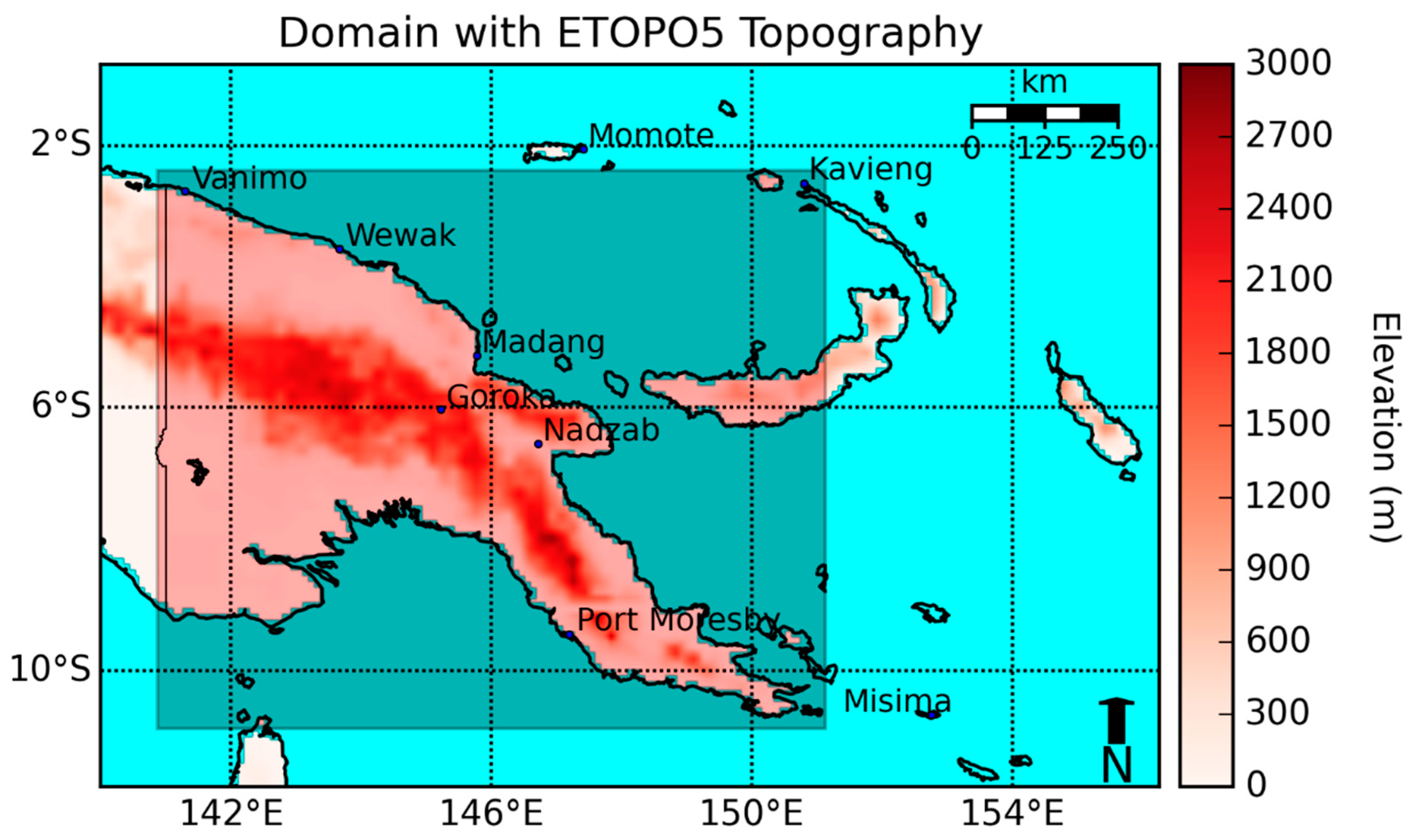
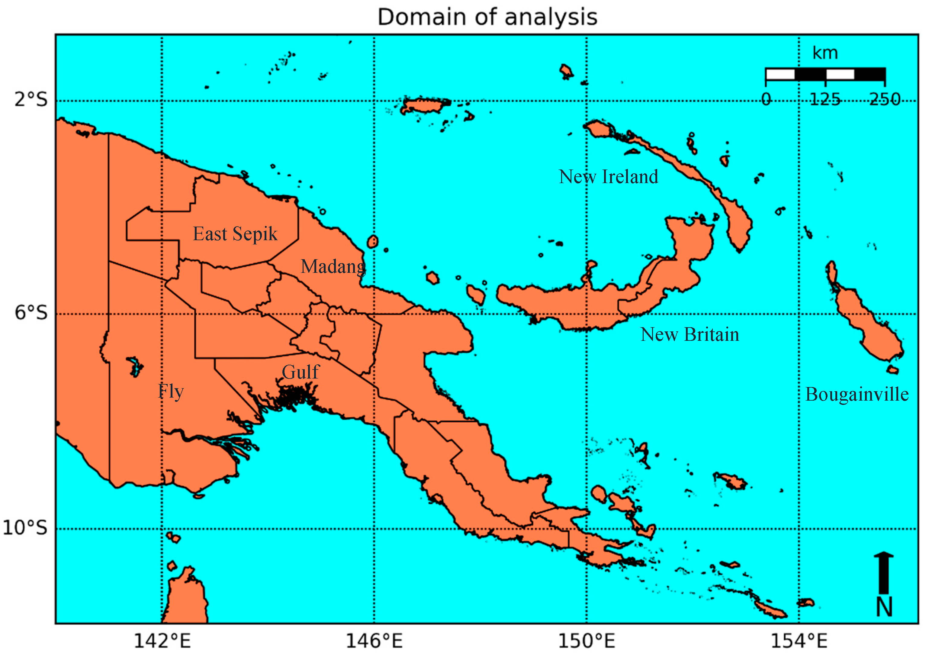
2.1. Study Area

PNG has a land area of just over 450,000 km², with the New Guinea Highlands running the length of the mainland [16]. The highest peak in the country is Mount Wilhelm at 4509 m (14,800 ft) [17]. Tropical rainforest covers most of the land [18]. The climate is tropical with a strong monsoonal influence [3]. However, the highest peaks of the country experience snowfall, one of the few locations close to the equator to experience this [17].

Much of PNG experiences a seasonal cycle in rainfall consisting of a wet and a dry season. This is largely due to the influence of the West Pacific Monsoon, also known as the Indonesian-Australian Monsoon, which results in moist north-westerly flow over the region during the wet season and drier south-easterly flow during the dry season [19]. For example, Port Moresby on the south coast demonstrates this seasonal pattern with over 75% of the average annual rainfall falling between November and April [3]. The broad-scale seasonal pattern is also affected by its proximity to significant orography and the coast, as well as the interplay with the Intertropical Convergence Zone and the South Pacific Convergence Zone, meaning seasonality is less marked in some locations, such as over New Britain [19,20].

For this study, a domain with a latitude range from the 0° to 12°S and a longitude range from 140°E to 156.5°E was selected for the gridded comparison (Figure 1). A map showing regions referenced in this study is included in Appendix A. The northern tip of Australia and western edge of the Solomon Islands are included in this domain but the impact of these two land areas on overall results can be considered negligible as they comprise only a small percentage of the entire domain. The data over the ocean were masked for the analysis. The topography map in Figure 1 is derived from NOAA’s ETOPO5 bedrock data, which models land topography and ocean bathymetry at a 5 arc-minute resolution [21].

2.2. Datasets

2.2.1. Validation Study

Satellite datasets used in this study are GSMaP and CMORPH. Access to the data was provided by JAXA and CPC/NOAA respectively through the WMO SWCEM Demonstration Project.

The version of GSMaP used was GSMaP Gauge-adjusted Near-Real-Time (GNRT) Version 6, which is adjusted using the gauge-calibrated version (GSMaP gauge) from the past period. The GSMaP gauge itself is calibrated by matching daily satellite rainfall estimates to CPC Unified Gauge-Based Analysis of Global Daily Precipitation (CPC Unified), a global gauge analysis [22]. Further details are contained in the GSMaP technical documentation [22].

Two versions of CMORPH were evaluated. These were the Bias-Corrected CMORPH (CMORPH CRT) and the Gauge-Blended CMORPH (CMORPH BLD) versions. The CPC Unified analysis is again used for bias correction over land but a different algorithm where estimates are matched to probability distribution function (PDF) tables from the past 30 days is employed. The Bias-Corrected version is used as a first guess for the Gauge-Blended version with further adjustment coming from the incorporation of gauge data based on observation density; further details can be found in literature produced by the developers [11,23].

The reference dataset for the gridded comparison was the ERA5 reanalysis produced by the European Centre for Medium-Range Weather Forecasts (ECMWF). A climate reanalysis is a numerical representation of meteorological fields created by combining meteorological observations with climate models. ERA5 is generated from 4D-Var assimilation of data into the ECMWF’s Integrated Forecast System (IFS) [24]. Only precipitation estimates from satellites and radar are assimilated [24].

Spatial and temporal details of the gridded datasets are shown in

Table 1. Details of the precipitation datasets used. CMORPH BLD and CMORPH CRT refer to the blended and corrected versions of the Climate Prediction Center Morphing Technique datasets; GSMaP refers to the Global Satellite Mapping of Precipitation dataset; and ERA5 refers to fifth generation ECMWF reanalysis.

Dataset	Resolution (°)	Start Time of Datasets	Latitude Range (°)	Longitude Range (°)
CMORPH BLD	0.25	January 1998	(−45, 40)	(50, 200)
CMORPH CRT	0.25	January 1998	(−45, 40)	(50, 200)
GSMaP	0.10	April 2000	(−45, 40)	(50, 200)
ERA5	0.25	January 1979	Global	Global

.

For the point-based comparison, precipitation data from nine meteorological observation stations operated by the PNG National Weather Service were used (the locations of the stations are shown in Figure 1.

A period from January 2001 to December 2018 was chosen as it is the longest common period across the datasets using full years.

2.2.2. Case Study for the 2015–2016 El Niño-Induced Drought

Six satellite-derived variables were used in the case study—GSMaP rainfall and GSMaP standardized precipitation index (SPI) from JAXA; NDVI, vegetation health index (VHI), and soil moisture and outgoing longwave radiation (OLR) from NOAA. A brief description of each of these variables follows.

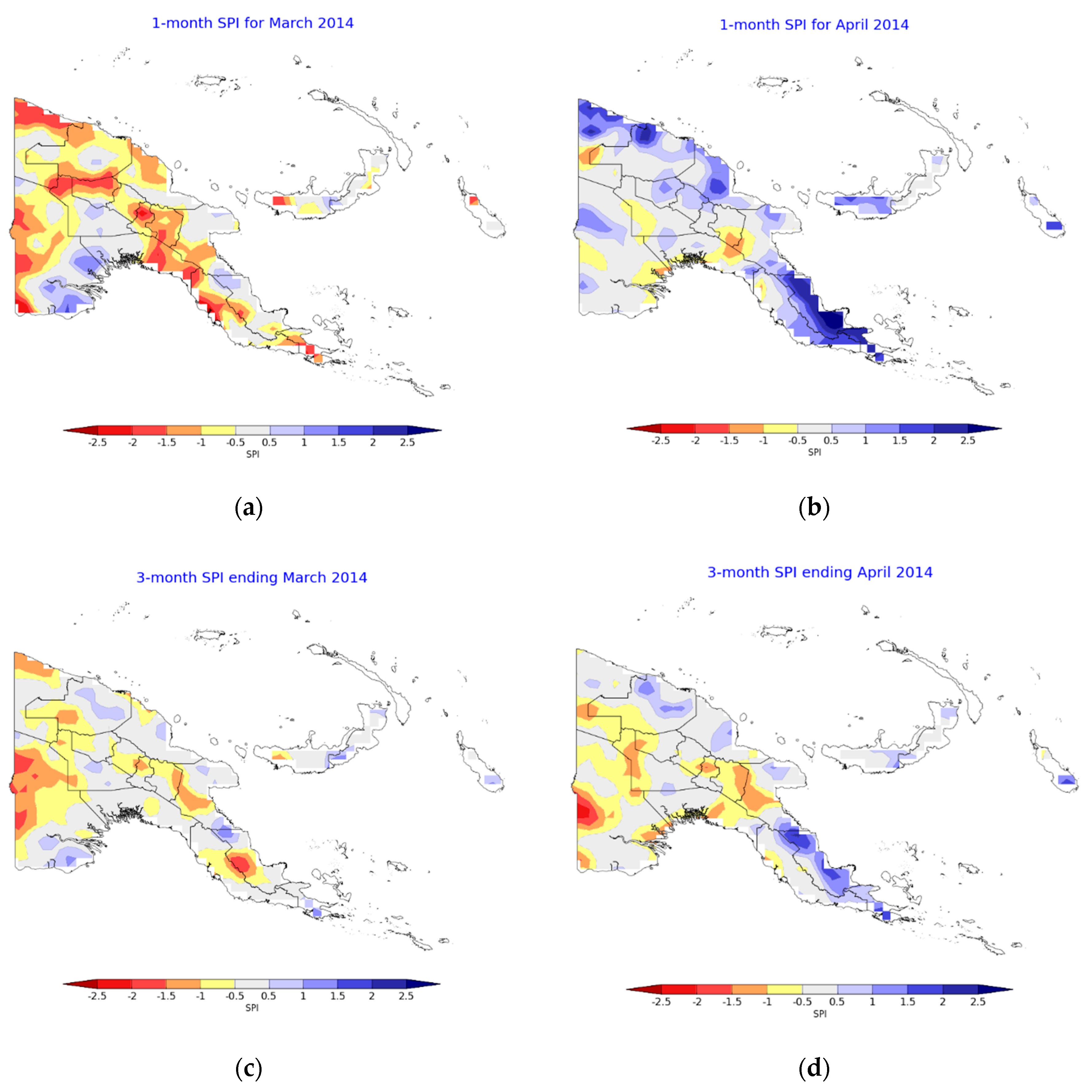
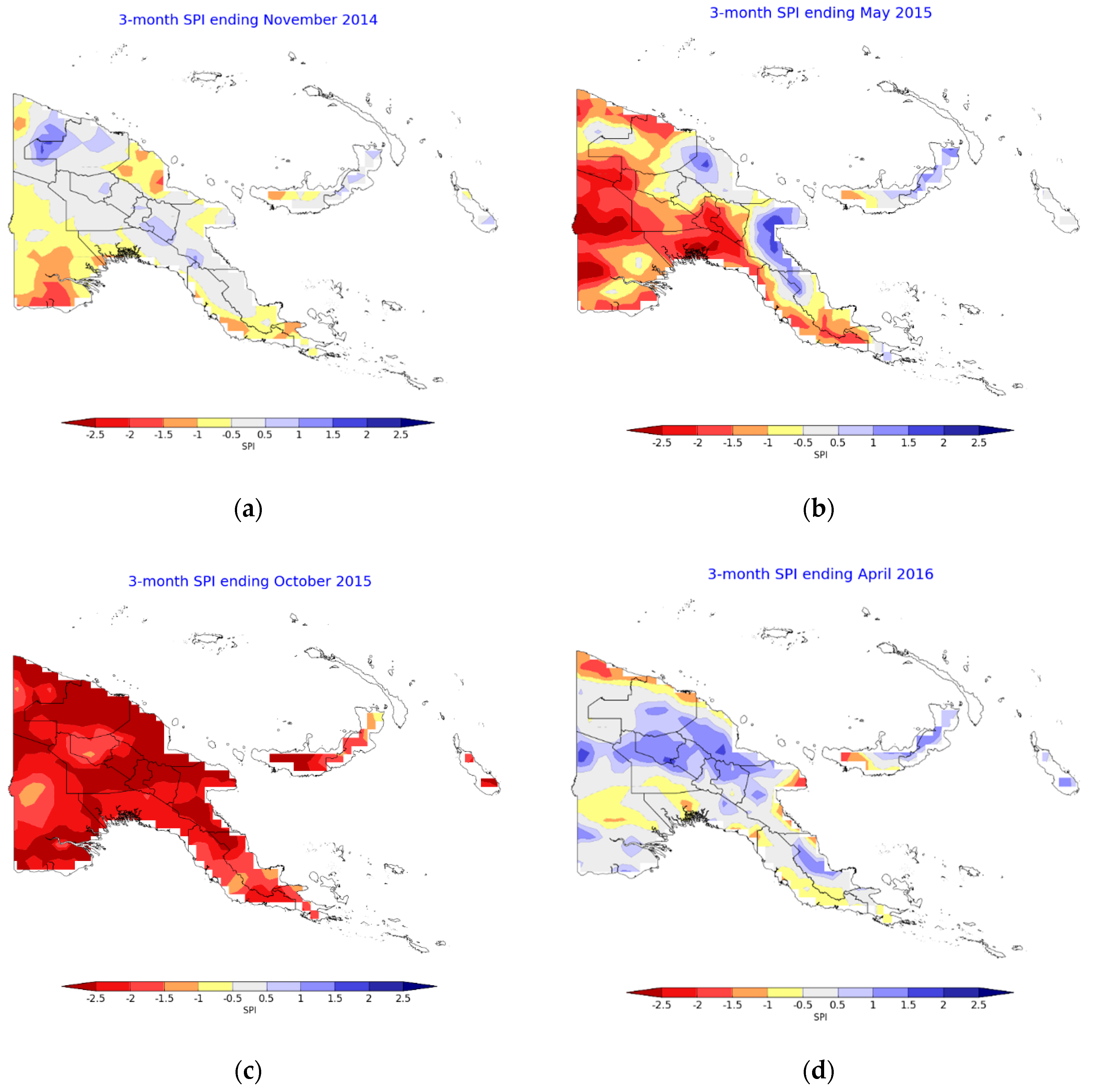
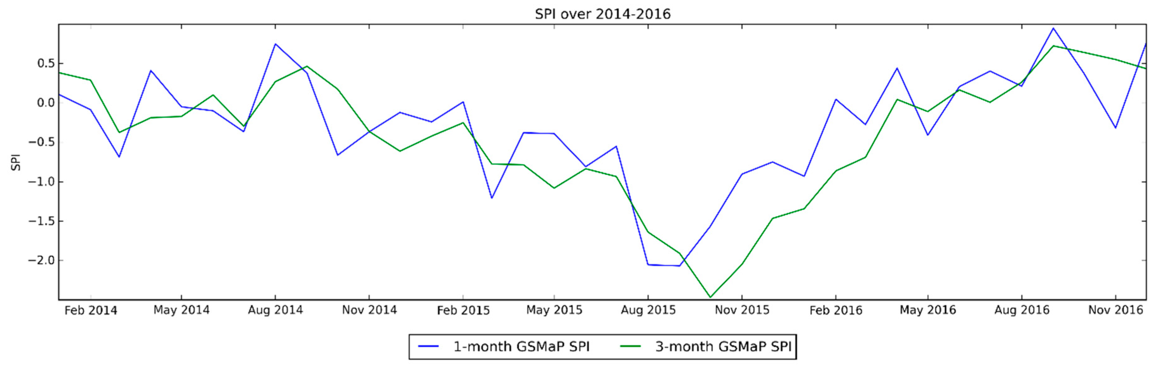
• The SPI is a commonly used index to characterise drought. It compares how different the rainfall observed is to the average for that period by measuring the number of standard deviations it is away from the mean [25]. Typically, values below −1.5 are considered “severely dry,” those below −2 are considered “extremely dry,” while values above 2 are indicative of “extremely wet” conditions [25,26].
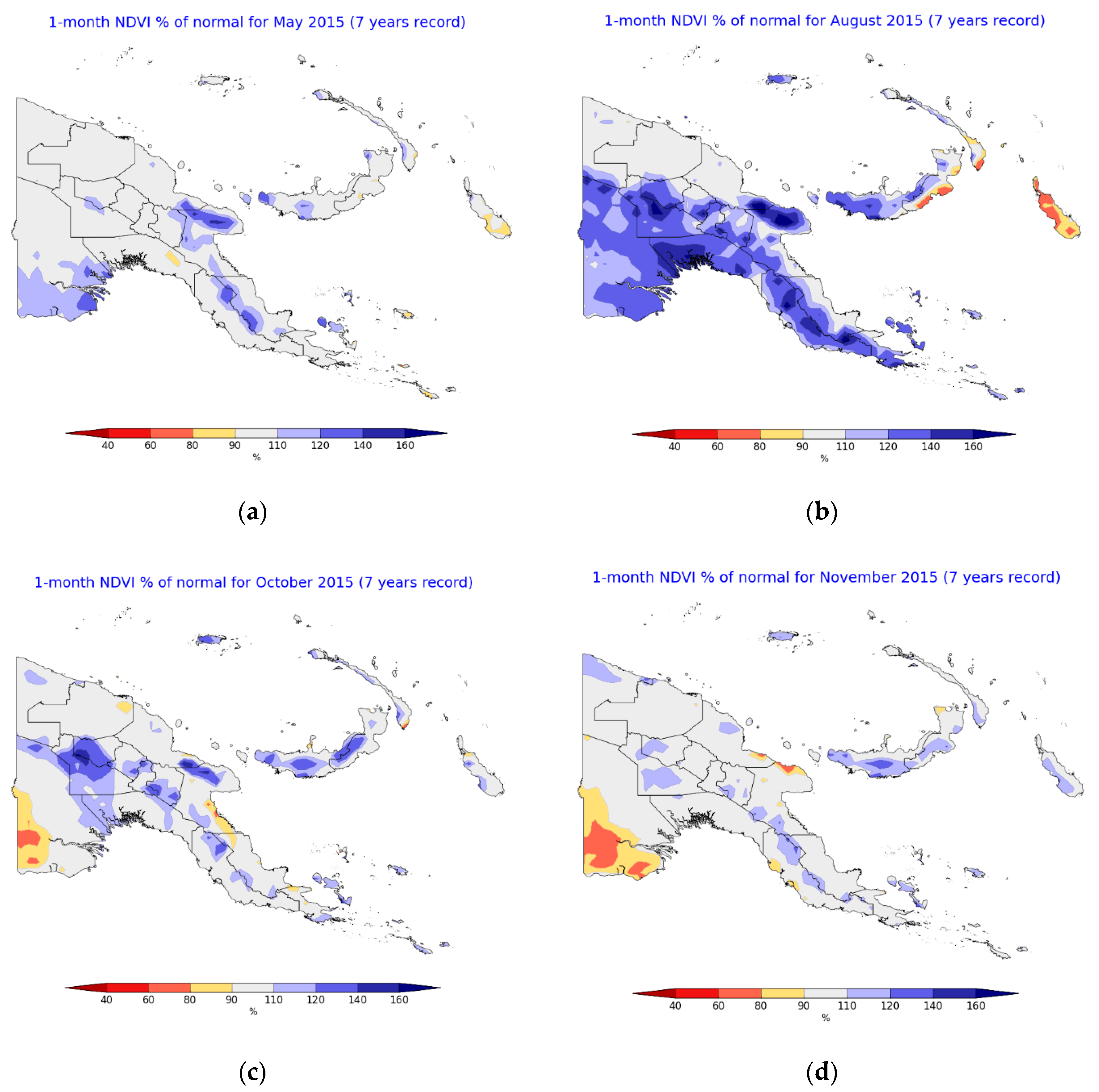
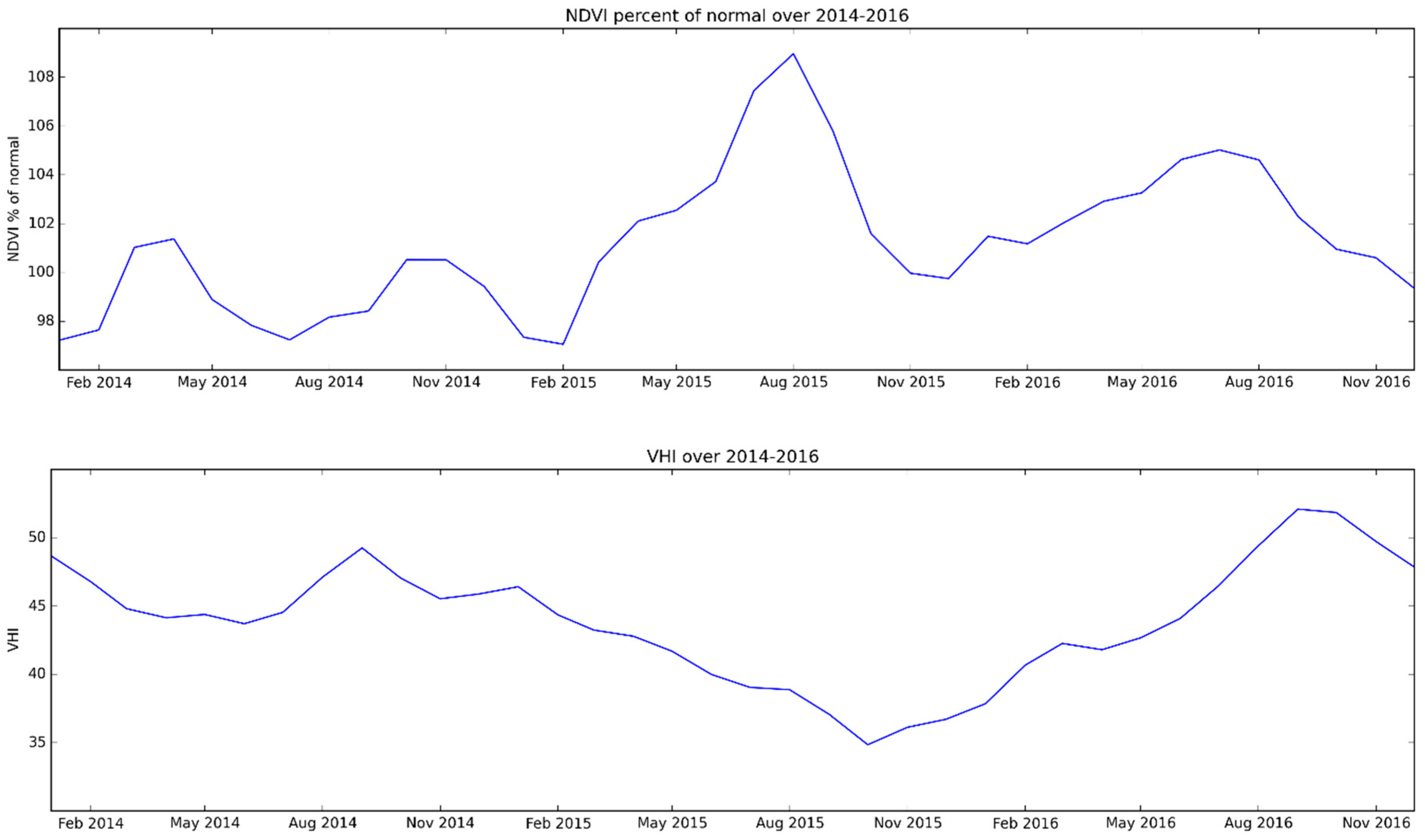
• The NDVI is a measure of the photosynthesis in vegetation. The NOAA AVHRR satellite instrument can measure visible (VIS) and near-infrared (NIR) radiations reflected from and emitted by the surface [27]. The NDVI is calculated based on the difference in intensity between these two wavelengths. This difference is then normalised by the sum of the intensities of wavelengths [27]. Soils do not demonstrate much difference between the two wavelengths while a large difference is taken to be indicative of dense green vegetation.

The equation for NDVI with ρ_NIR being NIR radiation and ρ_VIS being visible radiation:

$$NDVI=\frac{{\rho }_{NIR}-{\rho }_{VIS}}{{\rho }_{NIR}+{\rho }_{VIS}}$$

(1)

NDVI anomalies can be a possible indicator of drought by providing an estimate of whether photosynthesis in plants is above or below average. In an environment where photosynthesis is limited by the presence of water, wet (dry) conditions would lead to above (below) average photosynthesis and thus a positive (negative) NDVI anomaly. However, the relationship is complex and growth could also be impacted by other factors such as temperatures and cloud cover, though the variance of these variables over a tropical region like PNG is less than that of rainfall [27]. Furthermore, in a wet environment which is forested, the impact of rainfall reductions might not be as readily visible and so a decrease in photosynthesis (and the associated NDVI anomaly signal) would lag climate variables.

3.

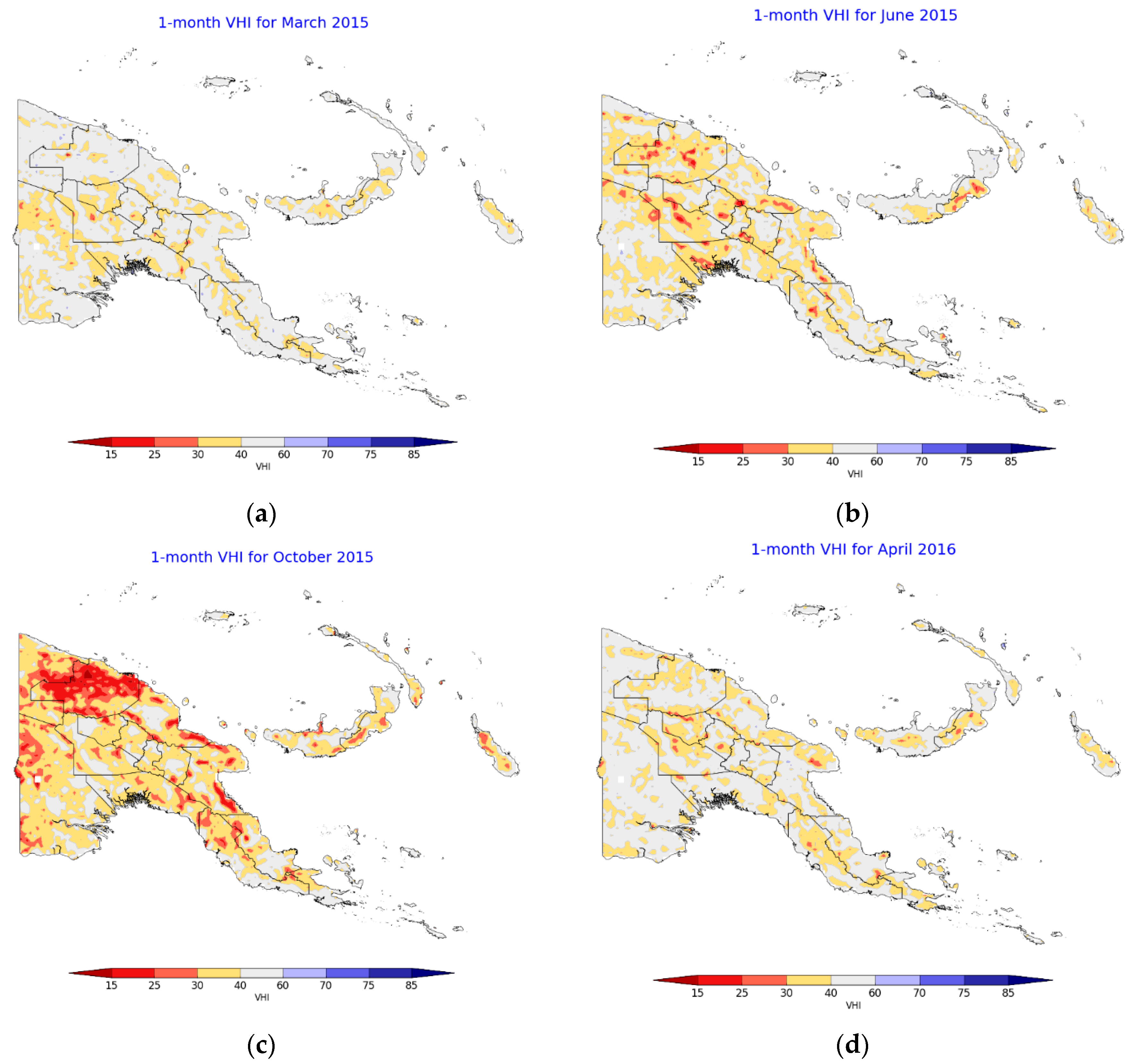
The VHI is another index that characterises plant health. It is composed of the Vegetation Condition Index (VCI) and the Temperature Condition Index (TCI). The VCI is NDVI normalised by its climatological range while the TCI is the land surface temperature (LST) normalised by its climatological range. The equation for VHI along with its components are shown below.

The equation for VHI:

$$VHI=\alpha \times VCI+\left(1-\alpha \right)\times TCI$$

(2)

The parameter α is a coefficient that determines the relative importance of VCI and TCI. It is typically taken as 0.5 to give equal weighting to the VCI and TCI: The parameter α is a coefficient that determines the relative importance of VCI and TCI. It is typically taken as 0.5 to give equal weighting to the VCI and TCI.

The equation for TCI:

$$TCI=\frac{LS{T}_{max}-LS{T}_{obs}}{LS{T}_{max}-LS{T}_{min}}$$

(3)

The equation for VCI:

$$VCI=\frac{NDV{I}_{obs}-NDV{I}_{min}}{NDV{I}_{max}-NDV{I}_{min}}$$

(4)

An inverse relationship is assumed between the VCI and the TCI with the assumption being that VCI decreases and TCI increases for poor vegetation health. High temperatures are known to have a negative impact on plant growth and thus are a potential indicator of vegetation stress [28]. R Cámara-Leret et al. (2019) found that under a 2 °C climate change temperature increase scenario, the geographic range of 63% of endemic plant species across the New Guinea island would be expected to decrease [29]. This relationship breaks down in regions where growth is energy- or sunlight-limited, which tends to be observed in the high latitudes and evergreen forests, scenarios which are less relevant to PNG [30].

Previous studies have taken VHI values below 30 to be indicative of drought [31,32]. As the VHI is already composed of normalised values, direct values of the index can be used for monitoring drought. Values above (below) 50 indicate wet (dry) conditions through increased (decreased) vegetation growth.

4.

Outgoing longwave radiation (OLR) is a measure of energy emitted to space by Earth’s surface and atmosphere and is a component of the radiation budget [33]. It can act as a proxy for clouds and rainfall as clouds reduce the amount of radiation that can be detected [34]. Normalised anomalies can be used as an indicator of drought with positive OLR anomalies being indicative of increased clear and dry conditions and negative OLR anomalies being indicative of increased clouds and rainfall.

The High Resolution Infrared Sounder (HIRS) uses multispectral regression models to measure the daily mean outgoing longwave radiation flux at the top of the atmosphere. It has been operational since 1998 and has been shown to be more accurate than the older AVHRR OLR that is also provided as a SWCEM product [35,36]. Consequently, this study is focused on the HIRS product.

5.

Soil moisture plays an important role in energy and water exchange between the surface and the atmosphere. Satellite-derived estimates of soil moisture are based on using microwaves to measure the emissivity of the surface and then linking this to conductivity and moisture [37]. Irrigation in PNG is very limited with most crops being rainfed [38]. As a result, it is reasonable to expect that remotely-sensed soil moisture is indicative of natural soil moisture.

The Soil Moisture Operational Products (SMOPS) is one example of a remotely-sensed soil moisture product and is available as a SWCEM product. Algorithm details are described in NOAA’s algorithm theoretical basis document [37]. Normalised anomalies may be an indicator of drought with a negative (positive) soil moisture anomaly indicating dry (wet) conditions.

2.3. Method

2.3.1. Validation Study

A gridded and point-based comparison was completed between the satellite datasets and the reference datasets. The GSMaP dataset was bilinearly extrapolated to 0.25° to allow values at each grid box to be directly compared across the datasets. For the point comparison, a bilinear interpolation was performed on gridded datasets from which a value corresponding to the co-ordinate of a station could be obtained. This value was then compared to the actual station value.

We have computed the mean bias (MB), root-mean-square-error (RMSE), mean average error (MAE) and the Pearson correlation coefficient (R). By dividing the MAE and MB by the average rainfall, these normalised versions remove the effect of higher rainfall averages, leading to larger errors. The RMSE is more strongly affected by the size of the error than the MAE. These metrics are commonly used in the evaluation of satellite rainfall estimates [10].

Further details about the continuous metrics are shown in

Table 2. Summary of metrics used.

Metric	Equation	Range	Perfect Value	Unit
Mean bias (MB)	$\frac{1}{N}{\displaystyle \sum _{i=1}^N}\left(E_i-O_i\right)$	(−∞, ∞)	0	mm/day
Mean average error (MAE)	$\frac{1}{N}{\displaystyle \sum _{i=1}^N}|E_i-O_i|$	[0, ∞)	0	mm/day
Root-mean-square-error (RMSE)	$\sqrt{\frac{1}{N}{\displaystyle \sum _{i=1}^N}{\left(E_i-O_i\right)}^2}$	[0, ∞)	0	mm/day
Pearson correlation coefficient (R)	$\frac{{{\displaystyle \sum }}_{i=1}^N\left[\left(E_i-\overline{E}\right)\left(O_i-\overline{O}\right)\right]}{\sqrt{{{\displaystyle \sum }}_{i=1}^N{\left(E_i-\overline{E}\right)}^2}\sqrt{{{\displaystyle \sum }}_{i=1}^N{\left(O_i-\overline{O}\right)}^2}}$	[−1, 1]	1

with E_i representing the estimated value at a point or grid box i, O_i being the observed value and N being the number of samples (across the full domain and period).

The ability of the satellite data in capturing extremes (highest and lowest quintiles) was also assessed using hit rates across the full period of record. This is a valuable statistic, as although the satellites may demonstrate performance that is poor in terms of absolute values, they may still be able to produce estimates that are accurately ranked in relation to their own climatology. This would suggest that percentile-based products that possess skill could be generated from the satellite precipitation estimates. As part of the WMO SWCEM Demonstration Project, CPC/NOAA and JAXA already produce satellite-derived percentile-based products such as the SPI and rainfall values expressed as high-end percentiles.

To calculate the percentile of an observed month, it was first ranked against the same month but for all the different years across the verification period. The ranking was then converted to a percentile through the equation shown below where P is the percentile, R is the rank of the month, and N is the number of years in the verification period:

$$P=\frac{R-1}{N-1}\times 100$$

(5)

To compute the hit rate, every time a bottom or top quintile month was observed across any location, the corresponding value from the satellite dataset was compared. A success was recorded if the satellite-estimated value also registered in the same quintile as the reference dataset value, otherwise, a failure was recorded. Quintiles were chosen, as the satellite data record length was deemed too short for deciles with the use of quintiles providing greater differentiation of extreme values compared to terciles or quartiles.

2.3.2. Case Study for the 2015–2016 El Niño-Induced Drought

The spatial and temporal patterns of the six variables were investigated by visualising the datasets as maps and then analysing the series of maps across the drought period. Normalised anomalies, also known as a percentage of the normal values, were used for rainfall, NDVI, soil moisture, and OLR to represent the difference from climatology more clearly. SPI and VHI are already a form of normalised anomalies. The anomalies were calculated using climatological averages derived from the full satellite records available through the SWCEM Demonstration Project (18 years for GSMaP rainfall, GSMaP SPI and VHI; 7 years for NDVI and soil moisture; and 6 years for OLR).

To visualise the data, the raw NetCDF data for each variable was plotted as a contour field on a base map using Python. The plotting library used was Matplotlib. A linear interpolation was performed to obtain values in between the data points.

3. Results

3.1. Validation Study

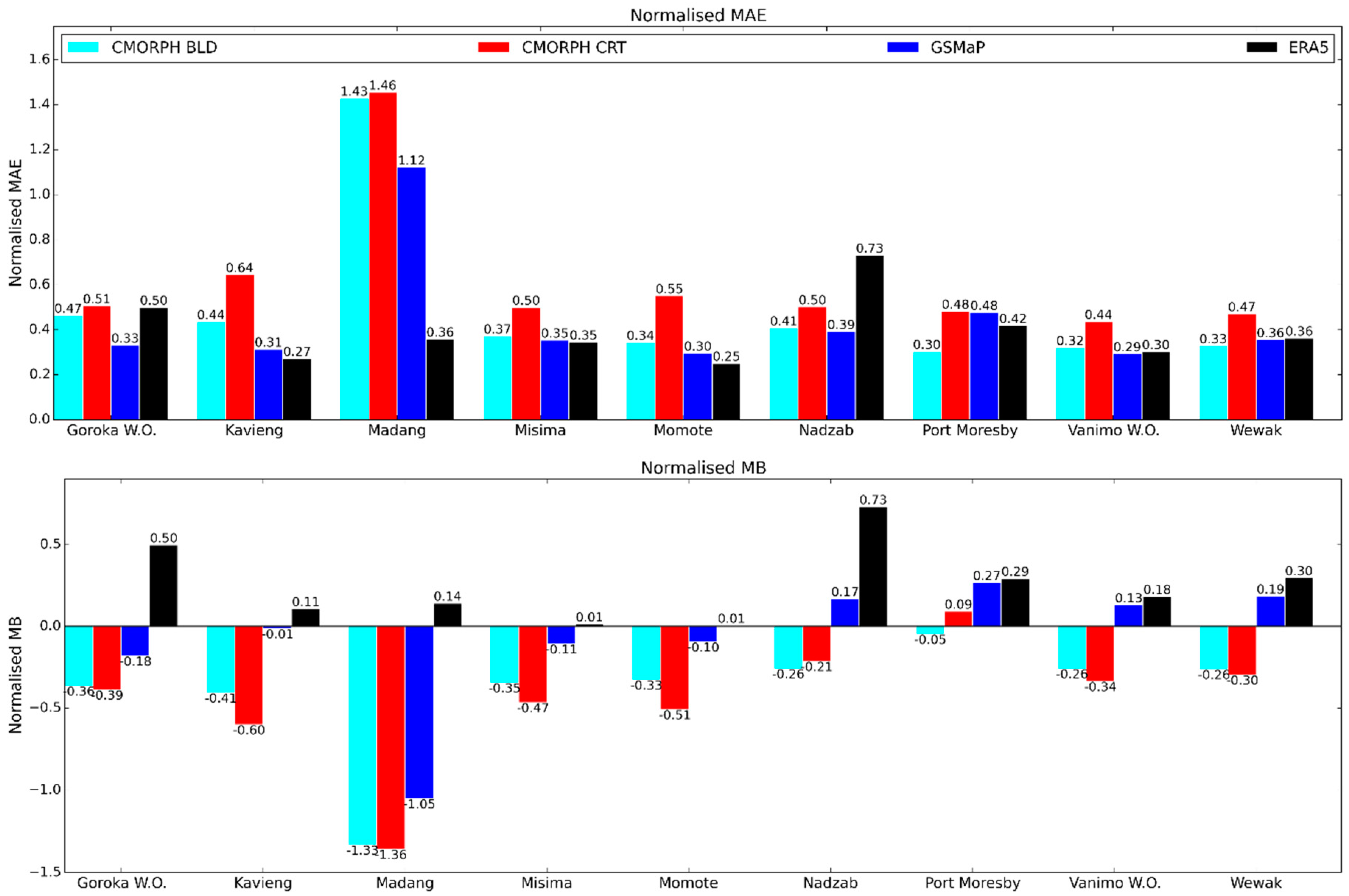
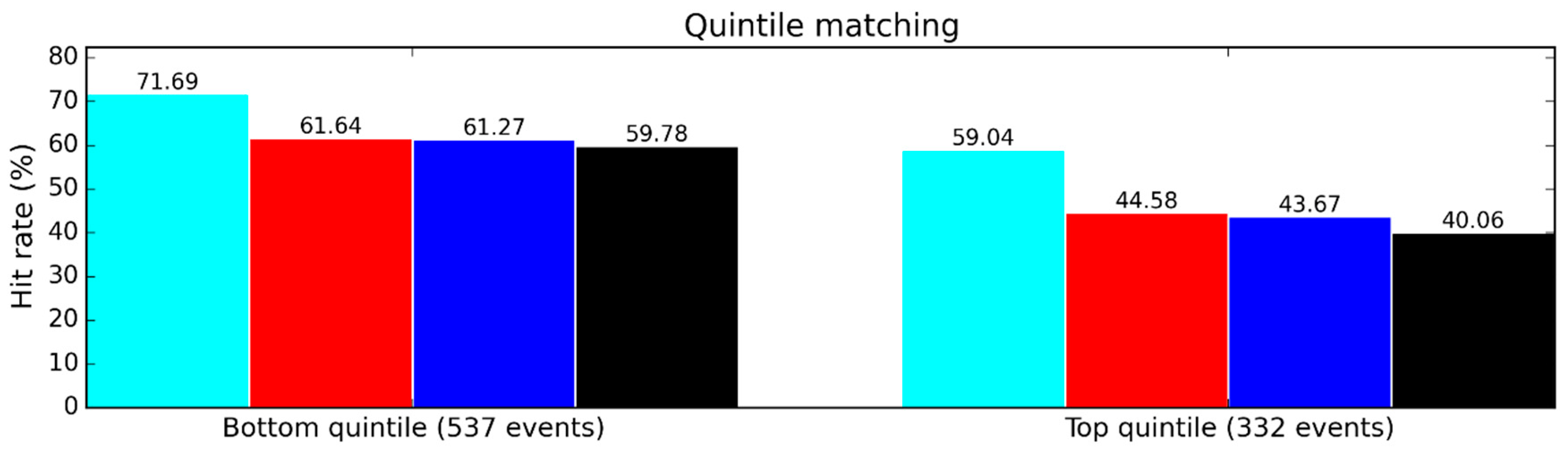
3.1.1. Point-Based Comparison

Figure 2 shows the normalised MAE and MB from the point-based comparison of the gridded datasets to the individual stations. In terms of the satellite datasets, GSMaP performed the best, followed by CMORPH BLD and then CMORPH CRT with the average normalised MAE of the nine stations analysed being 0.44, 0.49, and 0.62 respectively.

For reference, the average normalised MAE of ERA5 was 0.39, showing the bias of ERA5 was comparable to that of GSMaP and CMORPH BLD. However, the satellite datasets tended to underestimate rainfall at the stations while ERA5 overestimated it. As a result, when ERA5 is used as truth in the gridded comparison, it is expected that the error in the satellite datasets will be inflated. Performance of the satellite datasets was better than ERA5 at Goroka, which is the one station in this set where station elevation is significant (1572 m, with the next highest being Nadzab at 70 m).

The station-based quintile comparison also demonstrates skill, with the satellite datasets being able to detect bottom and top quintiles more often than not, as well as having better hit rates than ERA5. Performance is better for low-end totals which is the relevant metric for drought monitoring. If the metric was relaxed to simply test whether an observed bottom (top) quintile month was detected as a below-median (above-median) month according to the satellite, the hit rate improved to about 80% to 90% for the satellites, and 70% to 80% for ERA5.

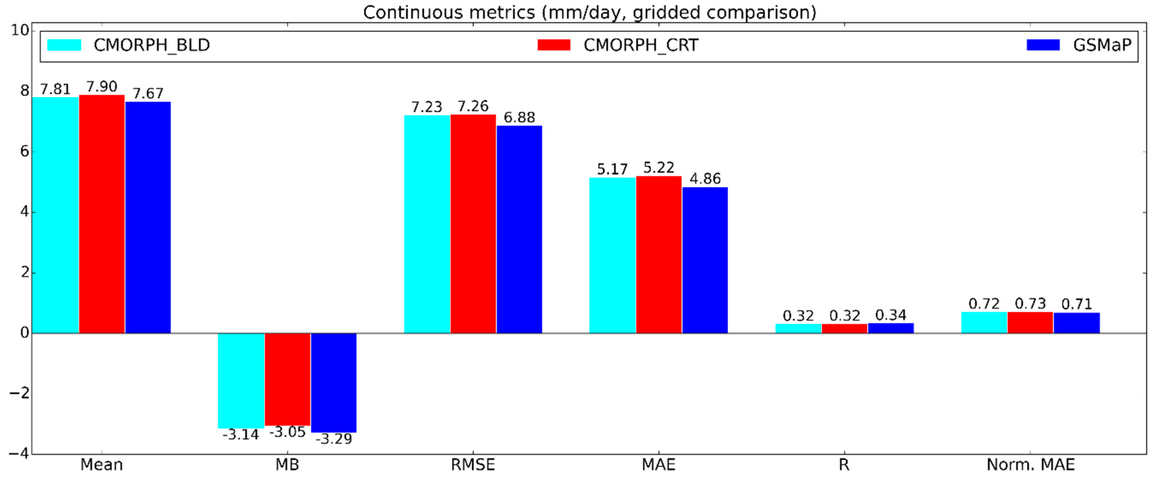
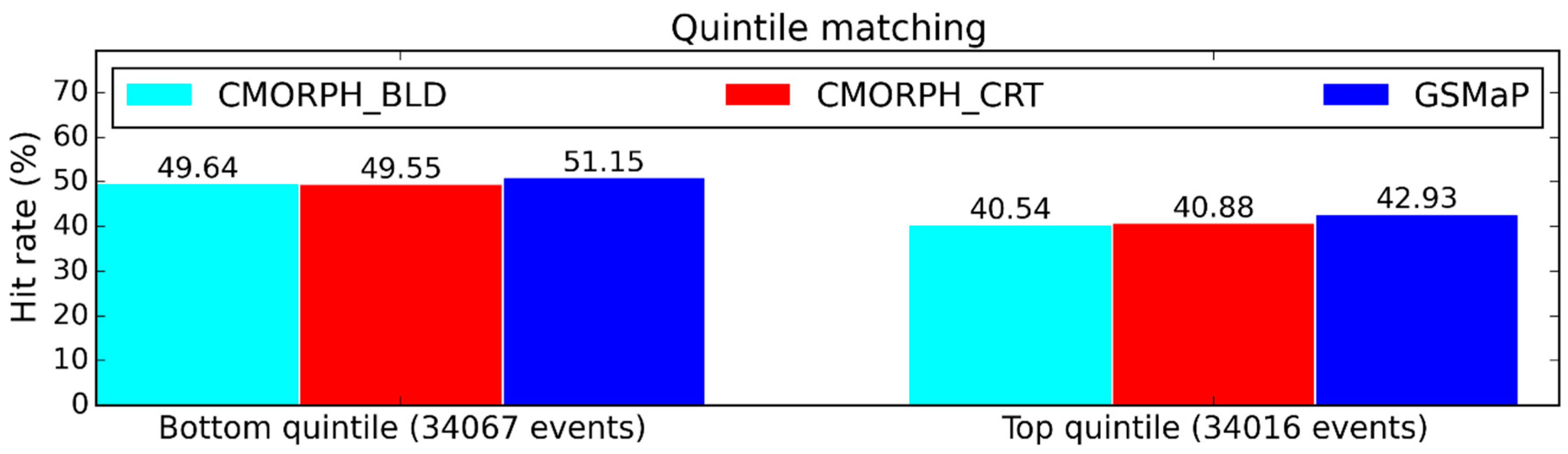
3.1.2. Gridded Comparison

Figure 3 shows the mean rainfall, MB, RMSE, MAE, and correlation co-efficient comparing the three satellite datasets with the ERA5 dataset over all the months from 2001–2018. This indicates that while all three datasets have similar values for all assessment scores, the datasets are generally too dry, and have differences from the observed gridded dataset that are about 70% of the average value. The satellites performed better in the point-based comparison than the gridded comparison. This is not surprising, as it was shown earlier in Section 3.1.1 that the ERA5 dataset has its own biases and it tended to overestimate rainfall while the satellite datasets underestimated it. ERA5 must assimilate from a limited number of observations itself, and hence will have large uncertainty in some areas which compounds the apparent error when it is used as “truth” in the gridded comparison. The absence of rain gauges over the region means it is difficult to quantify this error further than that achieved in the point-based comparison.

Using ERA5 as truth, the quintile comparison (Figure 4) shows the satellite-derived precipitation estimates could properly categorise low- and high-end events about 40 to 50% of the time. However, ERA5 was the worst-performing dataset in the quintile comparison using stations as truth, and so its ability to be used as truth in this metric is questionable at best.

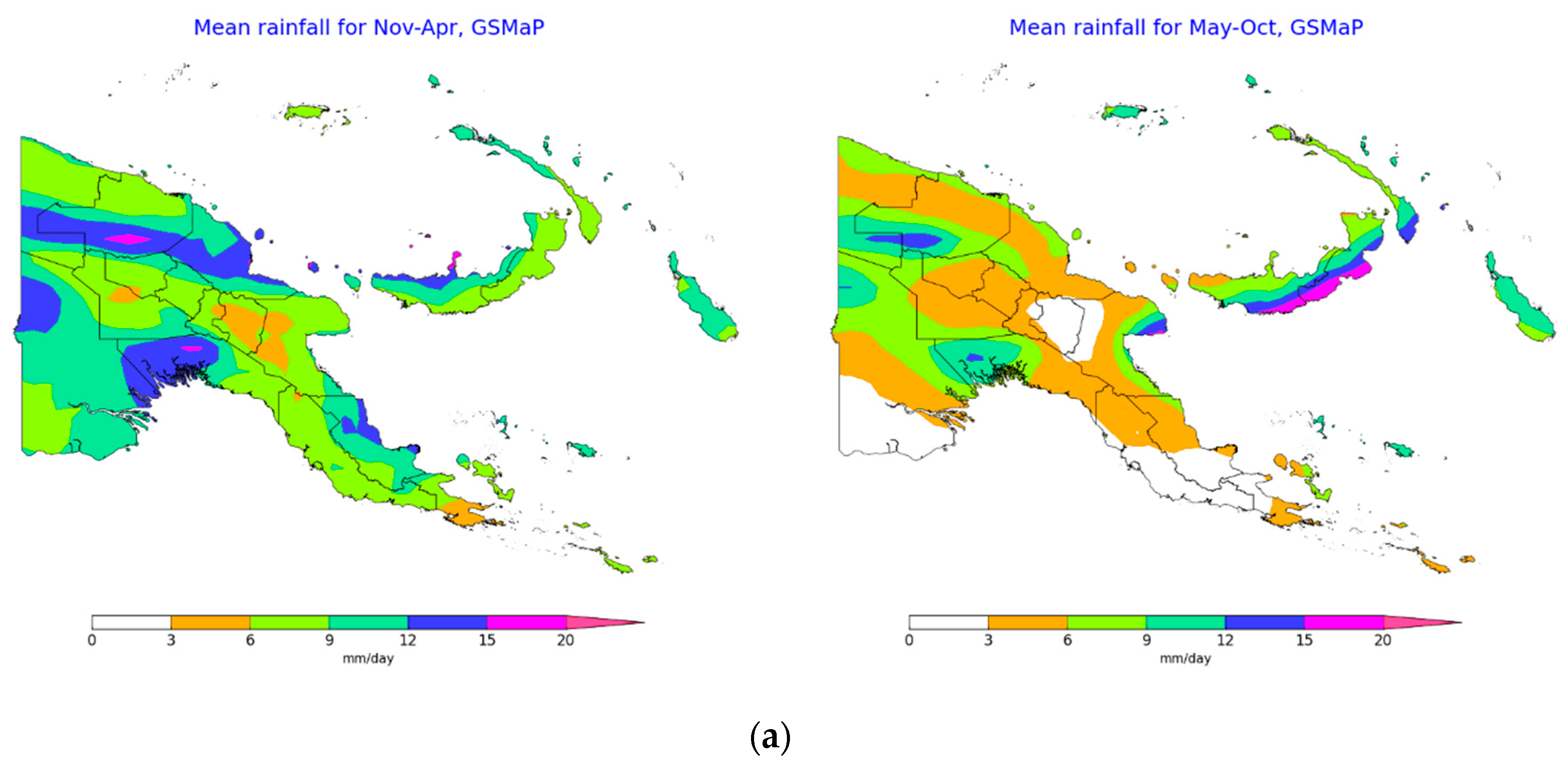
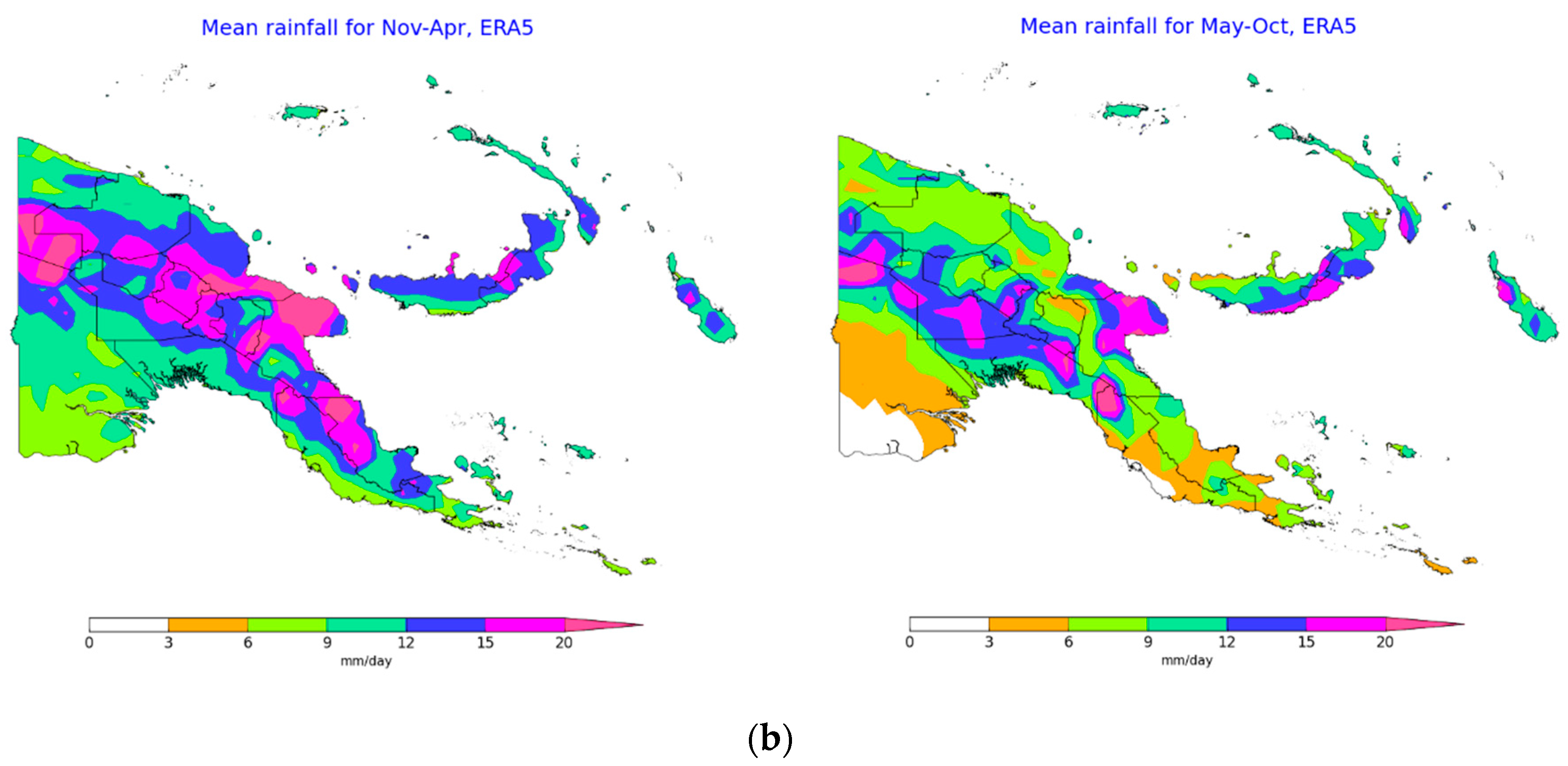
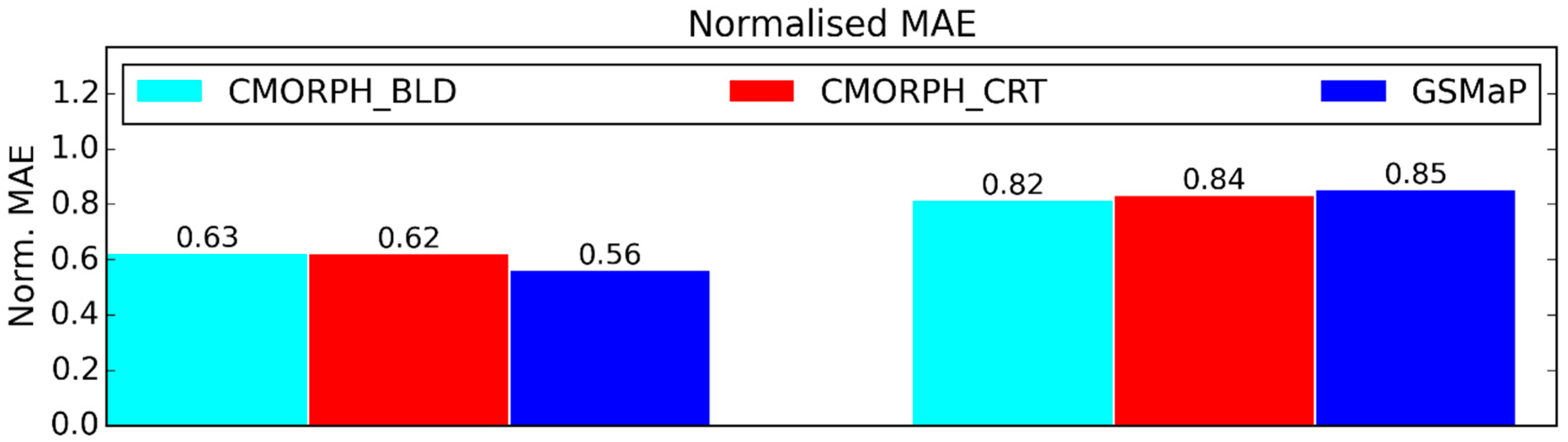
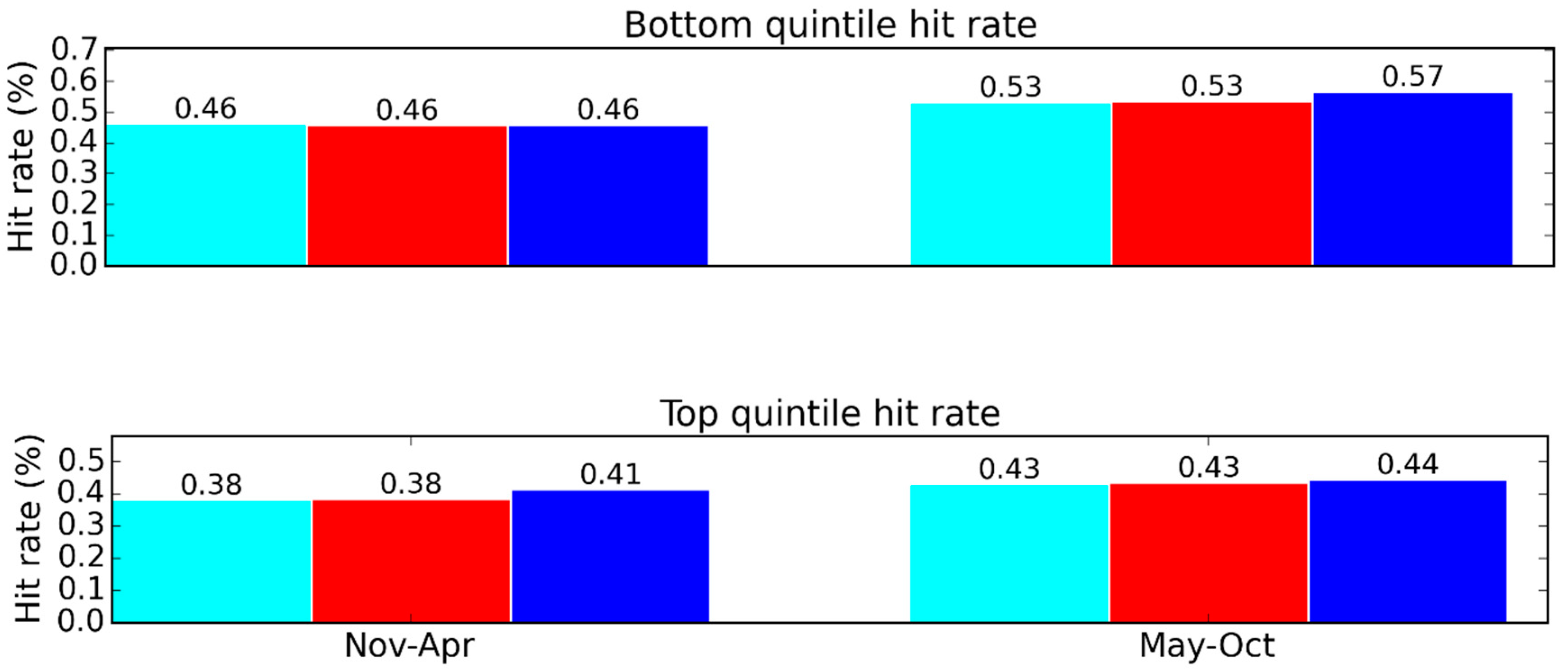
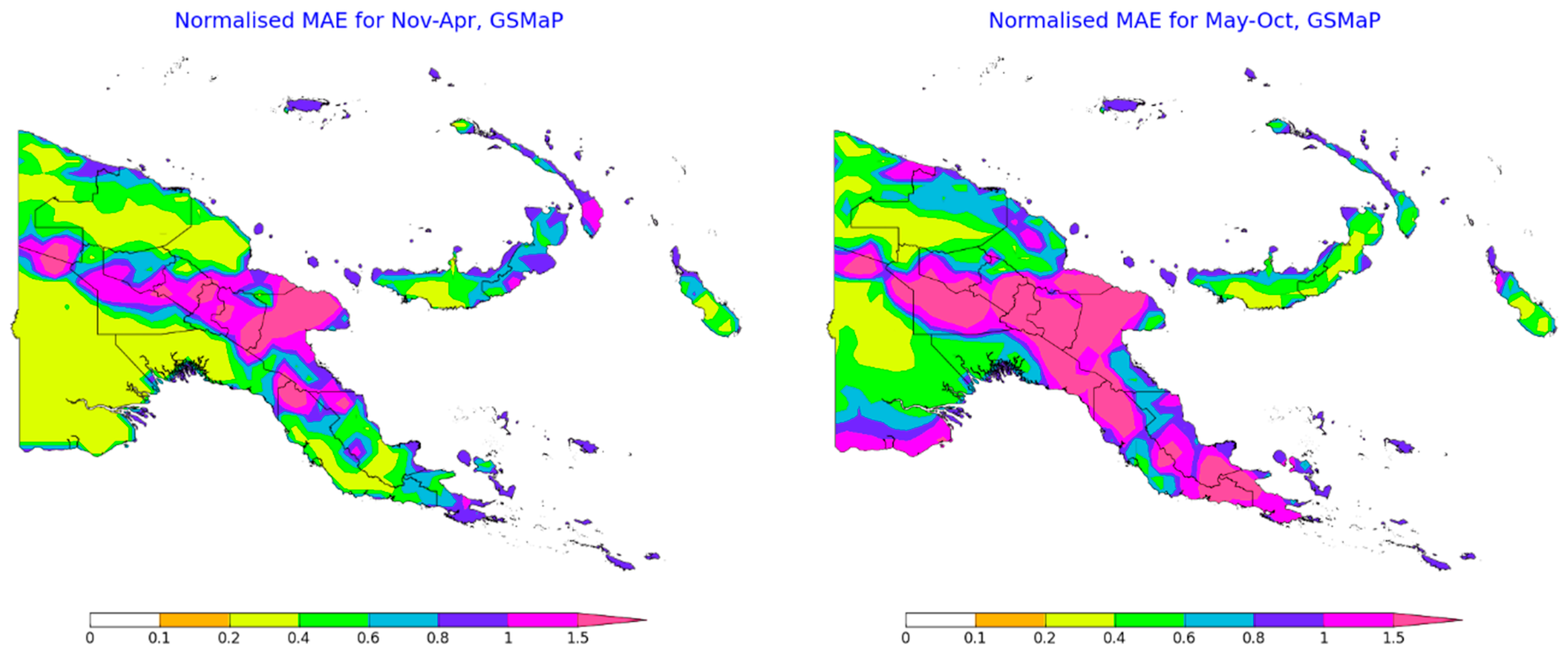
3.1.3. Seasonal and Geographical Comparison

To investigate the performance of the satellite-derived estimates across the two often distinct seasons in PNG, the dataset was split into a wet and a dry season based on the time of the year. Even though seasonality varies with geographical location as discussed in Section 2.1, the West Pacific Monsoon is the main seasonal driver for most of PNG and thus was used as the basis of this analysis. Consequently, the months from November to April were classified as wet while those from May to October were classified dry. Figure 5 illustrates the seasonal mean rainfall as estimated by GSMaP and ERA5. GSMaP data was chosen due to its slightly better performance over the other datasets.

For most of PNG, the use of November to April as the seasonal classification for the wet season is reasonable, with the exceptions being southern New Britain and southern New Ireland where the seasonality was reversed, and Bougainville where the seasonality was minimal.

Taking ERA5 as a representation of the truth, the general underestimation of rainfall as described in Section 3.1.1 is again apparent. Comparing Figure 5 to Figure 1, it is evident that the error tends to be the largest over the areas of highest topography, particularly over the New Guinea Highlands. Reasons for this will be given in Section 4.1. An important point is that as mentioned in Section 3.1.1, for the only station of significant elevation (Goroka), the satellite datasets performed better than ERA5 where the underestimation by the satellites was less than the overestimation by ERA5. This suggests that more generally, a positive bias in ERA5 over topography could exist, which would have compounded the satellite biases obtained when ERA5 was used as truth. The only case where overestimation occurs notably was in parts of the southwest of the country during the wet season.

The performance of the estimates was best over the Fly province, a region where the topography is relatively even and low. Interestingly, the high rainfall totals over the south coast of New Britain during the “dry” season (which rival those seen over the Highlands during the wet season) appear to be well-represented by GSMaP, the only case shown where a high-end rainfall total was accurately estimated by GSMaP. The normalised MAE and quintile hit rates averaged over the domain and categorised by seasons, are shown in Figure 6.

Figure 6 demonstrates that the error was smaller during the wet season. The hit rates for the quintile comparison are similar across the seasons, with the dry season exhibiting slightly better performance. The spatial representation of the normalised MAE is shown in Figure 7.

The performance of GSMaP is notably decreased during the dry seasons over the Papuan Peninsula, and towards the coasts of the Western Fly, Madang, and East Sepik provinces. Conversely, during the wet season, performance is decreased over southern New Ireland and the eastern half of New Britain.

The seasonal reductions in performance for these regions correspond to decreased rainfall for that particular region and season. This again alludes to a connection between low rainfall rates and reduced satellite monitoring performance, noting that mean rainfall was lower over south New Ireland and east New Britain during the months defined as wet in this study.

3.2. Case Study for the 2015–2016 El Niño-Induced Drought

A very strong El Niño event in 2015 and 2016 resulted in widespread drought, frost in the Highlands, and ultimately food insecurity across PNG. The peak intensity of the drought was declared by the PNG National Weather Service late in 2015. In a meteorological context, the drought eased in many areas in 2016 as rainfall returned to closer to average values late in 2015, but social impacts were still felt in some areas until early 2017 [39]. In this section, various SWCEM products are presented, and their usefulness in evaluating the spatial and temporal characteristics of the drought event is analysed. Both GSMaP and CMORPH provide the rainfall percentages of normal and the SPI. For this case study, the GSMaP version has been selected due to its marginally better performance, as demonstrated in Section 3.1.

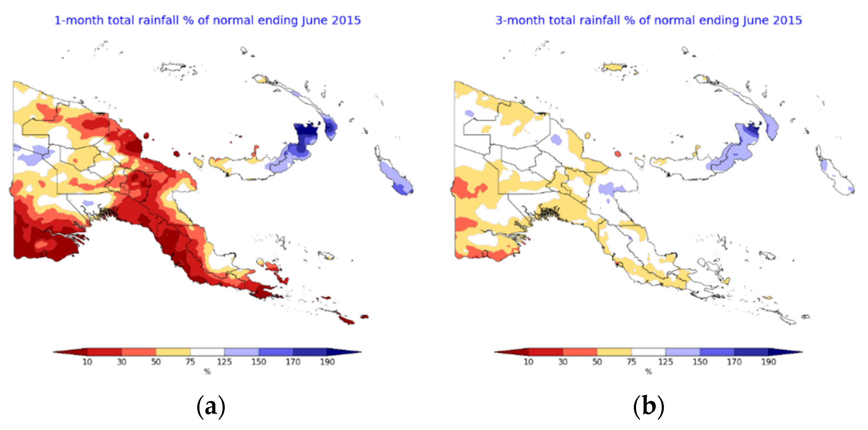
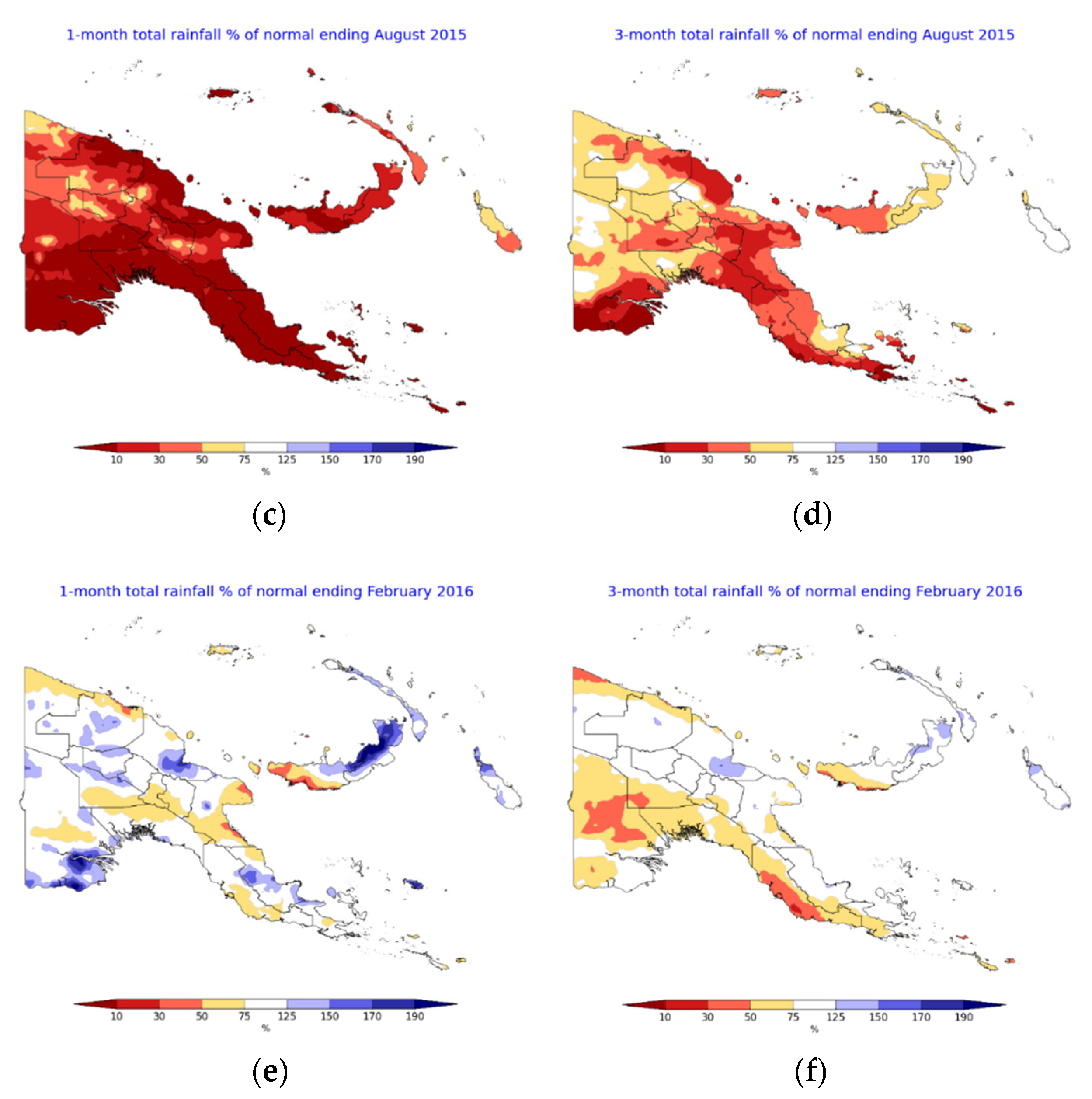
3.2.1. Rainfall

The rainfall percentages of normal were able to capture the onset of the drought by detecting a continuous period of widespread well-below average rainfall (e.g., less than 10% of the average) starting in June 2015 (Figure 8a,b), peaking around August 2015 (Figure 8c,d) and easing by February 2016 (Figure 8e,f). However, outside of the drought event, the rainfall percentages of normal also displayed a large amount of variance. For example, examining the spatial distribution of the rainfall percentages of normal for the second halves of 2014 and 2016 (maps not shown), areas where the rainfall was less than 10% of the average were also evident. Although not as widespread as during the peak of the 2015–2016 drought event, this indicates that using threshold values without considering spatial context would lead to false alarms and discretion is needed to ensure this is avoided.

It is important that the maps are examined in a series, especially if they are an average over multiple months. Both periods have their benefits as the 1-month anomaly provides a more rapid representation of the current state while multi-month aggregations such as the 3-month anomaly provide more insight into the longevity of conditions. This means that the 1-month anomaly can detect onset and cessation quicker, but the 3-month anomaly offers greater confidence in the continuity of the conditions.

3.2.2. Standardized Precipitation Index (SPI)

Using the 3-month SPI over the 1-month values of the index is recommended as it helps to smooth out short-term variations, reducing the prospect of a false alarm. For example, if the 1-month SPI for March 2014 is considered in isolation (Figure 9a), the values of the index could be indicative of drought conditions. However, the values of the 1-month SPI for April 2014 showed much wetter conditions (Figure 9b). On the other hand, the 3-month values of the SPI (Figure 9c,d) displayed significantly less variation in the values of the index and could be used more confidently for drought detection and monitoring. The resolution of the dataset was 0.25°.

Using the 3-month values of the index, it was demonstrated that the SPI was able to indicate that rainfall was anomalously low across the 2015–2016 drought period (Figure 10). The extreme values and the prolonged duration demonstrated the severity of the event.

The southwest of the mainland started showing notable and sustained conditions classified as “severely dry” (SPI values of −1.5 or below) from November 2014 (Figure 10a), while May 2015 marked the start of more severe and widespread drought (Figure 10b), with large parts of the country experiencing conditions classified as “extremely dry” (SPI values of −2 or below). The 3-month SPI identifies the peak as occurring around October 2015 (Figure 10c). These extremely dry conditions were seen to subside by April 2016 (Figure 10d). In terms of severity as indicated by the magnitude of the SPI, the first values below −2.5 were seen in March 2015, peaking in October 2015 and subsiding by April 2016. They were not seen elsewhere in the three years. The duration of the dry conditions as indicated by the SPI is in most cases more important than the severity given the sign can change quite frequently. The exception would be when very extreme values are obtained.

Continuous monitoring is required to track whether a month with anomalously dry conditions is indicative of a drought onset or whether it is a short-term rainfall deficiency that might soon ease. Nonetheless, examining the SPI maps revealed that the index was able to correctly identify the 2015–2016 drought event. The results are promising, and the 3-month SPI could be recommended as one of the indices to be used operationally for drought detection and monitoring.

3.2.3. Normalized Difference Vegetation Index (NDVI)

The normalised NDVI anomaly for several periods over the 2015–2016 drought is shown in Figure 11. The resolution of the dataset was 0.25°.

The normalised NDVI anomaly over the drought period does not clearly capture the dry conditions. The NDVI began to indicate green conditions starting from May 2015. In October 2015, which was correctly detected as around the peak of the event by the SPI and VHI, the NDVI showed largely neutral conditions. The driest conditions were depicted in November 2015, but the severity and extent were much less than that derived from rainfall. It could be reasonable that this timing was past the peak of the meteorological drought as a lag between vegetation growth and rainfall is expected. However, the lag observed was two to three months, which is quite large. In this situation, not only did the NDVI not indicate dry conditions during the peak of meteorological drought, it implied that vegetation was in good condition. The NDVI decreased from August 2015 to December 2015, after which it began to increase again, showing that although it does not seem to be useful for real-time detection of meteorological drought onset, it may still be useful for monitoring the cessation of drought effects on vegetation.

Outside of the drought event, it depicted dry conditions in July 2014 and wet conditions in August 2016 around the Gulf province. The former was somewhat consistent with the SPI while the latter was consistent with the VHI and SPI.

3.2.4. Vegetation Health Index (VHI)

The VHI for several periods over the 2015–2016 drought is shown in Figure 12. The resolution of the dataset was 0.1°.

It appears the VHI is a good indicator of drought in PNG. It correctly indicated poor vegetation growth over the drought period, depicting drought onset from June 2015, the worst drought conditions in October 2015, and cessation of drought by April 2016. The VHI did not show as widespread drought conditions as the SPI but it only showed significantly dry conditions over the true 2015–2016 drought period. This suggests that false alarms for the VHI is low and confidence in dry conditions being part of a longer-term drought event is higher than for the SPI. It is likely that LST responds more quickly to drought conditions than the NDVI, which would have a delayed response as described in Section 3.2.3, and so the inclusion of LST in the VHI allows it to be a more responsive indicator of drought conditions than using the NDVI alone.

3.2.5. Soil Moisture

The normalised soil moisture anomaly (figures not shown for brevity) indicated largely neutral conditions over much of the drought period. In October 2015, there were small areas of positive anomalies which were not consistent with the drought period. Even though it did depict some areas of below-average soil moisture, these were mostly towards the coast and not representative of the widespread drought experienced by the country.

3.2.6. Outgoing Longwave Radiation (OLR)

Positive OLR anomalies (figures now shown for brevity) began to appear from July 2015, linking up well with the beginning of the peak intensity of the drought. August to October 2015 also showed widespread positive anomalies. The anomalies returned to largely neutral values for November and December 2015, but then spiked to some of their highest values over the two years in January 2016 before returning to neutral values once again. The spike was concentrated towards the south. This was consistent with the SPI, which indicated an easing of drought conditions towards the north but the persistence of severe conditions towards the south during January 2016.

The normalised HIRS OLR anomaly product appears to have value in detecting droughts through a proxy of reduced cloud cover. During the severe portion of the drought period, positive OLR anomalies were apparent while the anomalies were neutral or negative outside of the drought period. Reduced cloud conditions resulted in frost in the PNG highlands, exacerbating the impact of dry conditions on food production.

3.2.7. Areal-Averaged Variables from 2014 to 2016

As the 3-month SPI is composed from the average of the 1-month SPIs from the last three months, the 3-month SPI plot represents a rolling-average, where variations that are smoothed are compared to the 1-month SPI plot.

Results presented in Figure 13 demonstrate that the SPI experienced a marked decrease after July 2015 though conditions were already drier than average from around February 2015. The decrease in the VHI was more gradual than that observed in the SPI. Conversely, the normalised NDVI anomaly increased from February 2015 to August 2015, indicating above average rates of photosynthesis even though this was a period of below-average rainfall. The normalised NDVI anomaly did decrease after August 2015 but its areal-averaged value was still above average. A possible explanation for this pattern could be that increased sunlight facilitated above average rates of photosynthesis before the severe rainfall deficit resulted in rates decreasing. Overall, this supports the results presented earlier which suggested that the SPI and VHI were more reliable indicators of drought for the 2015–2016 event than the normalised NDVI anomalies.

4. Discussion

4.1. Validation Study

Comparison of the point-based results for PNG to Australia indicates satellite performance at PNG is reasonable. For example, in Australia, an average normalised MAE of 0.28 and 0.54 for CMORPH BLD and GSMaP were obtained across a minimum of 4771 stations which compares to values of 0.49 and 0.44 at PNG stations [15]. This comparison is even more favourable when only tropical Australian stations (north of 23.5°S latitude) were considered, which yielded an average normalised MAE of 0.4 and 1.69 for CMORPH BLD and GSMaP across a minimum of 694 stations.

The gridded comparison demonstrated that the errors in satellite precipitation estimates across PNG can be large in some areas, especially over the mountainous regions. The poor performance of satellites over topography has been shown in earlier studies [9,14]. Cold surface contamination is unlikely to be the source of these large biases over PNG’s topography as snow only falls on the highest peaks in PNG and it would lead an overestimation of rainfall rather than the underestimation observed. Instead, this underestimation of rainfall is likely due to the poor ability of PMW satellites in detecting warm orographic clouds that are lacking in the ice particles which PMW detection is heavily reliant on [14]. The high spatial variance of rainfall across topography is likely to be another factor adding to the difficulty of satellite retrieval over such areas. The results from Goroka also suggested that ERA5 may have a positive bias over topography which would inflate the negative bias seen in the satellite datasets when ERA5 was used as truth.

The general underestimation of rainfall by satellites precipitation estimates over PNG found through this validation study is consistent with results from earlier studies suggesting that satellite observations tend to underestimate high-end rainfall totals [10]. One possible reason behind this is that the rapid evolution of convection is not observed between the successive satellite time steps. Underestimation is also compounded by poor detection of small rainfall totals due to the increased difficulty of detecting radiation changes from very light rainfall and the fact that light rain tends to fall from clouds with warmer tops, which satellites have difficulty detecting [10]. The weak performance of satellite precipitation estimates for very low rainfall rates is a likely reason why skill was considerably lower during the dry season [15,40].

However, the errors in the point-based comparison were less than for the gridded comparisons. This is likely due to the ability to calibrate the satellite precipitation estimates to station data at the numerous points analysed in this study. The elevation of the stations could also be a factor as eight of nine of the stations had an elevation of 70 m or less. However, the one remaining station with a significant elevation performed comparably to the lower-lying ones. The ability to calibrate and in the case of CMORPH BLD, adjust the satellite precipitation estimates against station data appears to improve the analyses. Although the limited rain-gauge network in PNG is a motivator for the use of space-based observations in this country, it is also a significant hindrance to obtaining accurate satellite precipitation estimates in areas that are a long distance from any gauge. This would suggest that any increase in the number of rainfall stations has the potential to greatly increase the accuracy of the satellite rainfall estimates. This is supported by results in past studies where areas with higher rain gauge density have exhibited significantly better performance [15]. The validation of this inference will likely be a basis for a future study.

4.2. Case Study for the 2015–2016 El Niño-Induced Drought

The VHI appears to be very useful for drought monitoring given its low propensity for false alarms and its correct detection of the onset, worsening and easing of the 2015–2016 drought. Users could feel confident that the indication of dry conditions was linked to a severe drought event. The SPI performed well in the detection of dry conditions, but its drawback was its erratic nature that could have caused false alarms. The use of the 3-month values of the index did eliminate some inconsistency in the SPI’s performance, though monitoring and discretion were still needed to determine if a dry signal was just a short-term blip or part of the more severe and longer-term event.

The normalised OLR anomaly appears to be another valuable indicator for drought detection. It displayed a widespread anomaly over much of the drought period. It also detected the easing of conditions in the north during January 2016. The magnitude of the anomaly was not large but there were also no false alarms over the study period.

Normalised rainfall anomalies detected the below-average rainfall of the 2015–2016 drought very well, but could potentially be too sensitive, as areas of significantly below-average rainfall were also detected outside of the drought event. If used in conjunction with the other indices, it would be a valuable tool for detection, as the maps are able to pick up the widespread areas of significantly below-average rainfall associated with drought. The 1-month anomaly is particularly useful for real-time monitoring.

The case study indicated that the normalised NDVI anomaly was a poor indicator for detecting and monitoring the 2015–2016 drought in PNG, incorrectly displaying good growth conditions over the drought period. This may be due to the small climatology record (7 years or less), though this factor did not hinder the OLR. Nonetheless, it is likely that with a longer climatology the effectiveness of all these indicators would be improved, especially the NDVI and OLR, since their climatology had to be computed from a shorter record than the VHI, SPI, and SMOPS products. The SPI and SMOPS products had their anomalies precalculated by CPC/NOAA, of which a longer climatology close to the full dataset record (20 years) can be assumed to have been used. The climatology for the other variables had to be calculated manually, with only 7 (6 for OLR) years of data being available at the time for use in this study. Given that one year was affected by a severe drought, this further decreases the reliability of this climatology. The rainfall in the remaining calendar years (2012–2018 excluding 2015) was around average.

The normalised soil moisture anomaly was also a poor indicator of drought in PNG. Even though it showed a dry anomaly during the start of the drought event, the spatial extent was not widespread and the deviation from the climatology was very low. This muted response means confidence in detection is lowered and false alarms are more likely. During the later stages of the drought, wet anomalies were indicated. Soil moisture detection through satellites is likely to be difficult in PNG where a considerable amount of the terrain is covered by dense rainforest that would hinder the satellite retrieval process.

Visualisation of drought information in the form of maps is valuable in assisting users to make their decisions. The selection of a colour scale is important in determining how severe the maps can appear as the variance during the drought event for each variable is different. In this study, different colour scales were used for each variable to display variance due to drought clearly while being insensitive enough to natural variance. Rainfall and VHI had the greatest responses, and so a neutral range from 75% to 125% and 40 to 60 respectively still allowed the anomalies to be evident. However, such a range did not work as well for the other variables and so a neutral range from 90% to 110% (95% to 105% for soil moisture) had to be employed. This suggests these variables do not change as much in response to drought and consequently might not be as good indicators. Changing the colour scale to be more sensitive to smaller anomalies allows the anomalies to be more evident, but may also lead to more false alarms.

5. Conclusions

The high dependency of PNG’s population and economy on rainfall along with the country’s vulnerability to extreme rainfall events has motivated the generation of a suite of satellite-derived precipitation products for use in the country via the WMO’s SWCEM Demonstration Project.

These products were validated in two parts: (i) a validation study of the precipitation estimates and (ii) a case study focusing on how well the SWCEM satellite-derived precipitation products represented the severe 2015–2016 drought in PNG.

Both a gridded comparison using ERA5 along with a point comparison using station data was undertaken. The results demonstrated that satellite-derived precipitation estimates may not have a high accuracy over most of PNG, with the normalised MAE being around 70% of the average rainfall. However, the accuracy of satellite precipitation estimates was significantly better at the stations with the normalised MAE, improving to around 40% to 50% of the average. It is possible that the improvement was a result of being able to calibrate the satellite-derived precipitation estimates to surface-based observation station data. Most of these stations were also along the coast, meaning biases due to variations in topography were also reduced. It is also probable that there is a considerable error away from the stations in the ERA5 reanalysis used as truth for the gridded comparison, and so the true error of the satellite precipitation datasets may not be as great as that obtained. It would be valuable if additional and independent station data could be used for the calibration of satellite estimates.

The second part of this study was focused on the ability of the satellite-derived products to capture the onset, peak, and cessation of the 2015–2016 El Niño-induced drought in PNG, along with its spatial extent. The VHI and OLR anomalies appear to be useful indices as they detected the onset, “peak,” and easing of the 2015–2016 drought. Their spatial representation was also extensive, consistent with reported impacts. The SPI and rainfall percentages of normal also appear to have value, though more discretion was needed in linking dry conditions to drought severity. Using a longer-aggregation period increases the confidence in the longevity of conditions. Soil moisture and the NDVI anomalies during the drought period did not show a clear “drought” signal, which suggests caution in their use with reference to other datasets.

Even though the satellite-derived precipitation estimates were not particularly skilful across most of the country, limitations of the current rain gauge network in PNG mean the information provided by satellites has value. The satellite-derived VHI, OLR, and SPI appeared to have more utility in monitoring the 2015–2016 drought than the satellite precipitation estimates as they gave a more definite depiction of the spatial and temporal evolution of the event.

The evaluation of satellite precipitation estimates (CMORPH and GSMaP) is an essential scientific contribution to WMO initiatives such as the Climate Risk and Early Warning Systems and the Space-based Weather and Climate Extremes Monitoring Demonstration Project which assist PNG, as well as other countries in Asia and the Pacific, with improving precipitation monitoring (including drought monitoring) [4,8].

References

- Ready for the Dry Years (2019). ST/ESCAP/2851. Available online: https://www.unescap.org/publications/ready-dry-years-building-resilience-drought-south-east-asia (accessed on 25 October 2020).
- McGree, S.; Schreider, S.; Kuleshov, Y. Trends and variability in droughts in the Pacific Islands and Northeast Australia. J. Clim. 2016, 29, 8377–8397. [Google Scholar] [CrossRef]
- Smith, I.; Moise, A.; Inape, K.; Murphy, B.; Colman, R.; Power, S.; Chung, C. ENSO-related rainfall changes over the New Guinea region. J. Geophys. Res.-Atmos. 2013, 118, 10665–10675. [Google Scholar] [CrossRef]
- Kuleshov, Y.; McGree, S.; Jones, D.; Charles, A.; Cottrill, A.; Prakash, B.; Atalifo, T.; Nihmei, S.; Seuseu, F. Extreme weather and climate events and their impacts on island countries in the western Pacific: Cyclones, floods and droughts. Atmos. Clim. Sci. 2014, 4, 803–818. [Google Scholar] [CrossRef]
- Kuleshov, Y.; Inape, K.; Watkins, A.B.; Bear-Crozier, A.; Chua, Z.-W.; Xie, P.; Kubota, T.; Tashima, T.; Stefanski, R.; Kurino, T. Climate Risk and Early Warning Systems (CREWS) for Papua New Guinea. In Drought–Detection and Solutions; IntechOpen: London, UK, 2020; pp. 147–168. [Google Scholar] [CrossRef]
- El Niño 2015/2016 Post Drought Assessment: Report of the Inter Agency Post Drought Assessment in Papua New Guinea September 2016 Papua New Guinea|ReliefWeb (n.d.). Available online: https://reliefweb.int/report/papua-new-guinea/el-ni-o-20152016-post-drought-assessment-report-inter-agency-post-drought (accessed on 21 January 2020).
- Cai, W.; Santoso, A.; Wang, G.; Yeh, S.-W.; An, S.-I.; Cobb, K.M.; Wu, L. ENSO and greenhouse warming. Nat. Clim. Chang. 2015, 5, 849–859. [Google Scholar] [CrossRef]
- Kuleshov, Y.; Kurino, T.; Kubota, T.; Tashima, T.; Xie, P. WMO Space-based Weather and Climate Extremes Monitoring Demonstration Project (SEMDP): First Outcomes of Regional Cooperation on Drought and Heavy Precipitation Monitoring for Australia and Southeast Asia. In Rainfall Extremes, Distribution and Properties; IntechOpen: London, UK, 2019; pp. 51–57. [Google Scholar] [CrossRef]
- Derin, Y.; Yilmaz, K.K. Evaluation of multiple satellite-based precipitation products over complex topography. J. Hydrometeorol. 2014, 15, 1498–1516. [Google Scholar] [CrossRef]
- Ebert, E.E.; Janowiak, J.E.; Kidd, C. Comparison of near-real-time precipitation estimates from satellite observations and numerical models. B Am. Meteorol. Soc. 2007, 88, 47–64. [Google Scholar] [CrossRef]
- Joyce, R.J.; Janowiak, J.E.; Arkin, P.A.; Xie, P. CMORPH: A Method that Produces Global Precipitation Estimates from Passive Microwave and Infrared Data at High Spatial and Temporal Resolution. J. Hydrometeorol. 2004, 5, 487–503. [Google Scholar] [CrossRef]
- Okamoto, K.; Ushio, T.; Iguchi, T.; Takahashi, N.; Iwanami, K. The Global Satellite Mapping of Precipitation (GSMaP) project. Int. Geosci. Remote Sens. Symp. (IGARSS) 2005, 5, 3414–3416. [Google Scholar] [CrossRef]
- Dinku, T.; Ceccato, E.; Grover-Kopec, E.; Lemma, M.; Connor, S.J.; Ropelewski, C.F. Validation of satellite rainfall products over East Africa’s complex topography. Int. J. Remote Sens. 2007, 28, 1503–1526. [Google Scholar] [CrossRef]
- Chua, Z.; Kuleshov, Y.; Watkins, A. Evaluation of satellite precipitation estimates over Australia. Remote Sens. 2020, 12, 678. [Google Scholar] [CrossRef]
- McVicar, T.R.; Bierwirth, P.N. Rapidly assessing the 1997 drought in papua new guinea using composite avhrr imagery. Int. J. Remote Sens. 2001, 22, 2109–2128. [Google Scholar] [CrossRef]
- Chepkemoi, J. Island Countries of the World. Available online: https://www.worldatlas.com/articles/which-are-the-island-countries-of-the-world.html (accessed on 29 November 2018).
- Bismarck Range|Mountains, Papua New Guinea|Britannica. (n.d.). Available online: https://www.britannica.com/place/Bismarck-Range (accessed on 24 January 2020).
- East Asia/Southeast Asia: Papua New Guinea—The World Factbook Central Intelligence Agency. (n.d.). Available online: https://www.cia.gov/library/publications/the-world-factbook/geos/pp.html (accessed on 16 November 2020).
- Smith, I.N.; Moise, A.F.; Colman, R.A. Large-scale circulation features in the tropical western Pacific and their representation in climate models. J. Geophys. Res.-Atmos. 2012, 117. [Google Scholar] [CrossRef]
- Chang, C.P.; Wang, Z.; McBride, J.; Liu, C.H. Annual cycle of Southeast Asia-Maritime Continent rainfall and the asymmetric monsoon transition. J. Clim. 2005, 18, 287–301. [Google Scholar] [CrossRef]
- Amante, C.; Eakins, B.W. ETOPO1 1 Arc-Minute Global Relief Model: Procedures, Data Sources and Analysis. NOAA Technical Memorandum NESDIS NGDC-24. March 2009; p. 19. Available online: http://www.ngdc.noaa.gov/mgg/global/global.html (accessed on 25 October 2020).
- Global Satellite Mapping of Precipitation (GSMaP) for GPM Algorithm Theoretical Basis Document Version 6. Available online: https://eorc.jaxa.jp/GPM/doc/algorithm/GSMaPforGPM_20140902 (accessed on 14 September 2019).
- Xie, P.; Joyce, R.; Wu, S.; Yoo, S.H.; Yarosh, Y.; Sun, F.; Lin, R. Reprocessed, bias-corrected CMORPH global high-resolution precipitation estimates from 1998. J. Hydrometeorol. 2017, 18, 1617–1641. [Google Scholar] [CrossRef]
- Hersbach, H.; Bell, B.; Berrisford, P.; Horányi, A.; Sabater, J.M.; Nicolas, J.; Dee, D. Global reanalysis: Goodbye ERA-Interim, hello ERA5. Ecmwf. Newsl. 2019, 159, 17–24. [Google Scholar] [CrossRef]
- Keyantash, J.; Dracup, J.A. The quantification of drought: An evaluation of drought indices. B Am. Meteorol. Soc. 2002, 83, 1167–1180. [Google Scholar] [CrossRef]
- Standardized Precipitation Index (SPI)|NCAR Climate Data Guide. (n.d.). Available online: https://climatedataguide.ucar.edu/climate-data/standardized-precipitation-index-spi (accessed on 21 February 2020).
- Measuring Vegetation (NDVI & EVI). (n.d.). Available online: https://earthobservatory.nasa.gov/features/MeasuringVegetation/measuring_vegetation_2.php (accessed on 21 January 2020).
- Karnieli, A.; Bayasgalan, M.; Bayarjargal, Y.; Agam, N.; Khudulmur, S.; Tucker, C.J. Comments on the use of the Vegetation Health Index over Mongolia. Int. J. Remote Sens. 2006, 27, 2017–2024. [Google Scholar] [CrossRef]
- Cámara-Leret, R.; Raes, N.; Roehrdanz, P.; de Fretes, Y.; Heatubun, C.D.; Roeble, L.; Hannah, L. Climate change threatens New Guinea’s biocultural heritage. Sci. Adv. 2019, 5, eaaz1455. [Google Scholar] [CrossRef]
- Karnieli, A.; Agam, N.; Pinker, R.T.; Anderson, M.; Imhoff, M.L.; Gutman, G.G.; Goldberg, A. Use of NDVI and Land Surface Temperature for Drought Assessment: Merits and Limitations. J. Clim. 2010, 23, 618–633. [Google Scholar] [CrossRef]
- Kogan, F. World droughts in the new millennium from avhrr-based vegetation health indices. Eos, Trans. Am. Geophys. Union 2002, 83, 557. [Google Scholar] [CrossRef]
- Yoon, D.-H.; Nam, W.-H.; Lee, H.-J.; Hong, E.-M.; Feng, S.; Wardlow, B.D.; Kim, D.-E. Agricultural Drought Assessment in East Asia Using Satellite-Based Indices. Remote Sens. 2020, 12, 444. [Google Scholar] [CrossRef]
- Outgoing Longwave Radiation (OLR): HIRS|NCAR Climate Data Guide. (n.d.). Available online: https://climatedataguide.ucar.edu/climate-data/outgoing-longwave-radiation-olr-hirs (accessed on 21 January 2020).
- Chelliah, M.; Arkin, P. Large-Scale Interannual Variability of Monthly Outgoing Longwave Radiation Anomalies over the Global Tropics. J. Clim. 1992. [Google Scholar] [CrossRef]
- Ellingson, R.G.; Hai-Tien Lee Yanuk, D.; Gruber, A. Validation of a technique for estimating outgoing longwave radiation from HIRS radiance observations. J. Atmos. Ocean. Technol. 1994, 11, 357–365. [Google Scholar] [CrossRef]
- Lee, H.T.; Gruber, A.; Ellingson, R.G.; Laszlo, I. Development of the HIRS outgoing longwave radiation climate dataset. J. Atmos. Ocean. Technol. 2007, 24, 2029–2047. [Google Scholar] [CrossRef]
- Jensen, K. (n.d.). Soil Moisture Operational Product System (SMOPS) Algorithm Theoretical Basis Document. Available online: https://www.ospo.noaa.gov/Products/land/smops/figures/SMOPS_ATBD_v3.0.pdf (accessed on 25 October 2020).
- Aquastat Country Profile Papua New Guinea; Food and Agriculture Organization of the United Nations: Rome, Italy, 2011.
- Evaluation of Australia’s Response to El Niño Drought and Frosts in PNG 2015-17 INL847. (n.d.). Available online: www.iodparc.com (accessed on 21 January 2020).
- Ning, S.; Song, F.; Udmale, P.; Jin, J.; Thapa, B.; Ishidaira, H. Error Analysis and Evaluation of the Latest GSMap and IMERG Precipitation Products over Eastern China. Adv. Meteorol. 2017, 2017, 1–16. [Google Scholar] [CrossRef]