1. Introduction
Nowadays, the main source of electrical energy for spacecrafts is the light energy of solar radiation. The conversion of light energy into electrical energy is carried out by solar panels, which consist of semiconductor photocells connected to each other. The significant dependence of the properties of semiconductor materials on temperature and light flux density leads to the fact that the intrinsic current–voltage characteristics of solar panels also depend on operating conditions. This dependence leads to inconsistency in the output voltage of the panels. At the same time, on-board equipment makes certain requirements for the quality of power supply. Since the use of solar panels in spacecrafts provides for the modes of direct connection of onboard equipment to them, the problem arises of regulating the output voltage of the panels in such a way that it is kept within specified limits with a wide, including abrupt change in the load current, luminous flux density, and temperature. The solution to this problem is assigned to the automatic control system for solar panels. Therefore, the development of methods for the synthesis of these controls systems and the analysis of their properties is an urgent task of space instrumentation.
Known studies in this area mostly consider the static characteristics of power supply systems and the issues of their optimization in terms of specific power. In particular, work [
1] considers the problem of automatically maintaining the maximum output power of solar arrays based on the simultaneous search for both the optimal voltage value on solar panels and their angular position in Euclidean space. The work [
2] solves the problem of constructing highly efficient voltage converters that provide extreme regulation of the power of solar panels in a wide range of changes in their operating conditions. In this case, the static volt–ampere and volt–watt characteristics of solar modules are used. In the paper [
3], for the design of solar arrays, the method of multipurpose optimization is applied, taking into account the static parameters of solar panels: maximum power, number of cells in the module, maximum voltage on the panel. In works [
4,
5], the associated problems of constructing control systems associated with the automatic orientation of the spacecraft and forecasting the modes of power consumption are solved. The paper [
6] provides an overview of methods for efficient use of solar arrays in conditions of unpredictable partial shading. In this case, the operation of the power supply system is considered in quasi-steady modes. In work [
7], which is the closest in terms of topics to this paper, solar panels is presented as a model of an ideal current source, i.e., its dynamic properties as the main element of the system—the control object—are not taken into account.
The aim of this work was to study the dynamic characteristics of the elements of the solar array control system, develop a general control algorithm for the system, and the synthesis of its regulator.
A general scientific result of the work is the proposed modular principle of constructing a control system with the organization of a hierarchical structure of interaction of solar panels. The implementation of this principle makes it possible to reproduce the homeostatic mechanism of functioning of biological organisms in the power supply system.
The applied results include the developed dynamic model of the solar panel, the analysis of which made it possible to establish that when the panel operates together with a shunt switch, a voltage resonance occurs in it. A method for eliminating the undesirable consequences of this resonance is proposed. A regulator of the control system was developed, and a study of its robust properties in relation to changes in internal parameters and external load parameters was carried out.
The paper is a development of work [
8] published within the framework of the conference “International Conference on Industrial Engineering, Applications and Manufacturing” (ICIEAM-2020).
The paper uses an inductive approach to the study, in which the results obtained in the analysis of particular, specific cases are discussed and then generalized to the level of general technical significance.
2. Analysis of the Structure of the Control System and Its Composition
We will consider the currently widespread shunt structure of the solar array control system,
Figure 1 [
9,
10]. Such a structure is adopted, for example, in Spacebus 4000 (Thales Alenia Space, France), Boeing 702HP (Boeing, USA), in the energy module of the International Space Station. The most important advantage of shunt control systems in comparison with systems with step-up converters is the high reliability of their operation, which is necessary primarily for spacecraft with a long autonomous flight time [
1]. Long-term operation of such devices is characterized not only by periodic changes in the illumination and temperature of photocells, but also by a significant degradation of the parameters of solar panels. The shunt control principle has proven itself well in control systems with low voltage (30 V) solar panels. However, the transition to high-voltage power supply systems for spacecrafts is currently underway [
11,
12]. Gallium arsenide batteries with a nominal voltage of 150–200 V, which are used in such systems, have a large internal capacity and noticeable inductance. The presence of these reactive elements significantly changes the dynamic properties of the solar panel and requires additional studies of these properties with the subsequent use of the results of these studies for the synthesis of the control system.
Let us briefly analyze the presented structure.
The load voltage
UL is controlled by a sensor –resistor attenuator, from which the signal
US(
t) is taken. The control system is based on the principle of regulation by the deviation of the signal
US(
t) at the sensor output from the required value
Ur(
t). The calculated error
ε(
t) =
Ur(
t)−
US(
t) passes through the proportional-integral controller and the correcting element. The received signal
Uc(
t) is fed to a pulse-width modulator, which controls an electronic switch (shunt). If, under the influence of varying load current
IL(
t), temperature
T(
t) of the solar cell, or illumination
W(
t), the voltage
UL(
t) deviates from the given one, then the pulse width of the shunt switch will change to such an extent to compensate for the influence of the disturbing effect and restore required value of load voltage. Thus, the ultimate goal of controlling solar arrays can be described by a generalized functional expression:
In accordance with the above description of the general principle of operation of the system, the following functional units and variables can be distinguished in it:
control object—solar panel and consumers of electrical energy;
controlled variable—load voltage UL(t);
control action—voltage Uc(t) at the input of the pulse-width modulator;
disturbing influences—load current IL(t), luminous flux density W(t), photocell temperature T(t);
regulator—proportional-integral link connected in series and, in general, an additional correction link;
the feedback on the controlled variable UL(t) is realized through the inertia-free voltage sensor.
When moving in a near-Earth orbit, the system operates under conditions of repeated and cyclic entry of the spacecraft into and out of the shadow zone. These transitions are accompanied by temperature drops of photocells from −110 to 80 °C and a significant change in the level of illumination of solar panels, including the mode of their partial shading.
The specified operating conditions of the system should be taken into account during its synthesis as standard conditions for its functioning.
3. Study of the Solar Panel as a Control Object
3.1. Mathematical Model
From the structure diagram shown in
Figure 1, it follows that the solar panel together with the load constitute the control object of the system, the properties of which are decisive for solving the synthesis problem. A typical approach to modeling solar panels is to reproduce their static current–voltage characteristics [
13,
14]. Since the dynamic properties of the object play an essential role in transient modes of operation of the control system, then to compile a mathematical model of the panel, we will take into account the reactive components in the equivalent circuit of its photocells,
Figure 2.
Designations in
Figure 2:
Ip—photocurrent (current source);
Iin—reverse current of the
p-n junction;
Rp—resistance of the photocurrent leakage circuit,
Rp = 1 × 10
5 Ω;
Cp—capacity of the photocell;
Rs—series resistance,
Rs = 0.002 Ω;
U—the output voltage of the photocell;
Rc and
Lc—resistance and inductance of field connections of the module;
I—load current;
V—voltage at the output terminals of the module.
Each module of the panel consists of Ns photocells connected in series (Ns = 60), and Np of these series chains connected in parallel (Np= 4). In turn, a solar panel is made up of several modules, which can be connected both in series and in parallel.
For the equivalent circuit shown in the figure, equations can be drawn up for currents and voltages connecting
I(
jω) and
U(
jω) in an implicit complex form [
8,
15]:
where
Iin.i—the initial value of the reverse current, A;
Isc.r—nominal short-circuit current,
Isc.r= 2.5 A;
q—the electron charge,
q = 1.602 × 10
−19 C;
Ur.i—nominal no-load voltage,
Ur.i = 176 V;
B—Boltzmann’s constant,
B = 1.381 × 10
−23 J/K;
A—coefficient correcting the calculated form of the current–voltage characteristic,
A = 6.3;
Wn—nominal value of the luminous flux density (illumination),
Wn = 1000 W/m
2;
Tn—nominal value of the photocell temperature,
Tn = 298 K;
k—temperature coefficient of photocurrent growth,
k = 0.002 A/K;
E—contact potential difference of the
p-n junction,
E = 0.4 V.
3.2. Study of the Static Characteristics of a Solar Panel
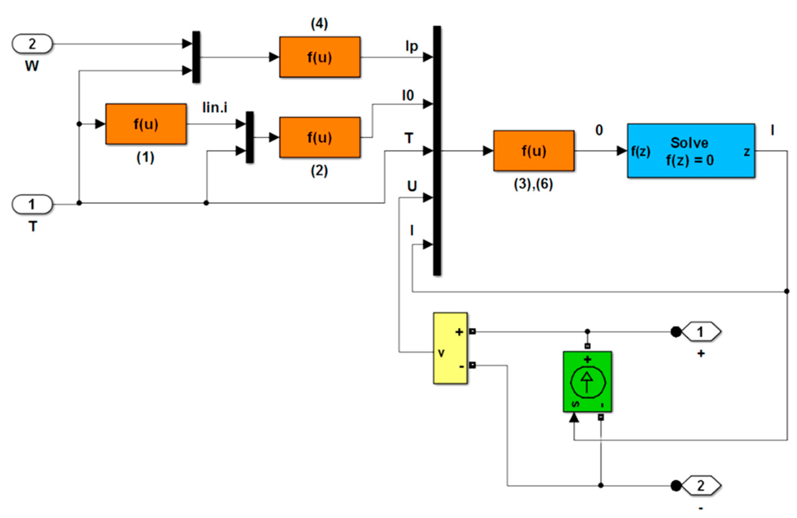
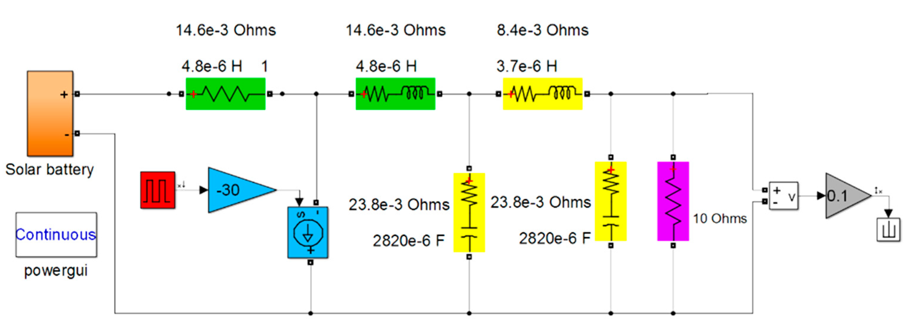
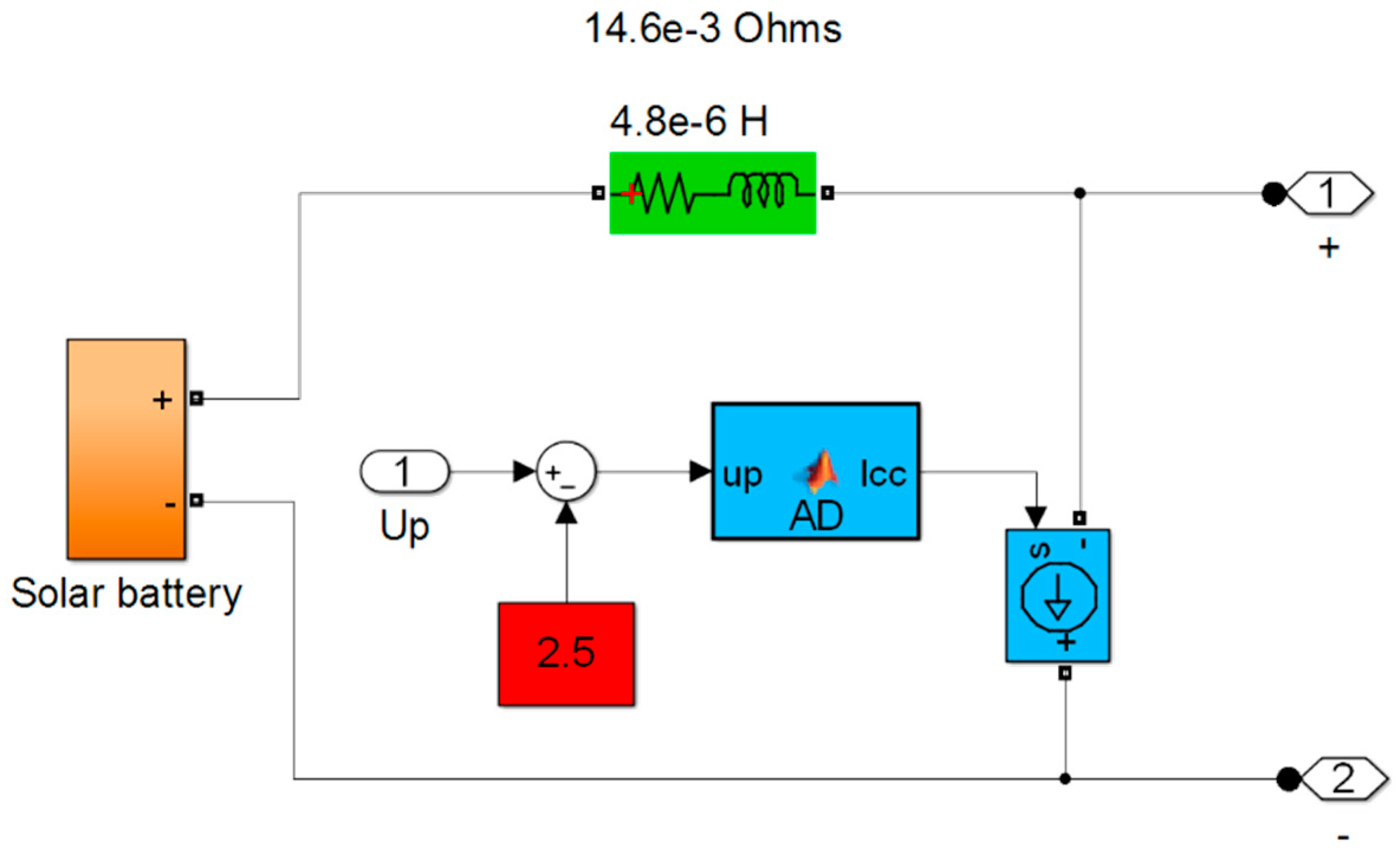
Let us consider a panel with three modules. To obtain its characteristics, a simulation model of the panel was built in the MatLab package,
Figure 3.
The scheme for solving Equations (2)–(7) in the cell blocks of the model is given in
Appendix A.
The numerical values of the solar panel parameters in the model are presented in
Table 1.
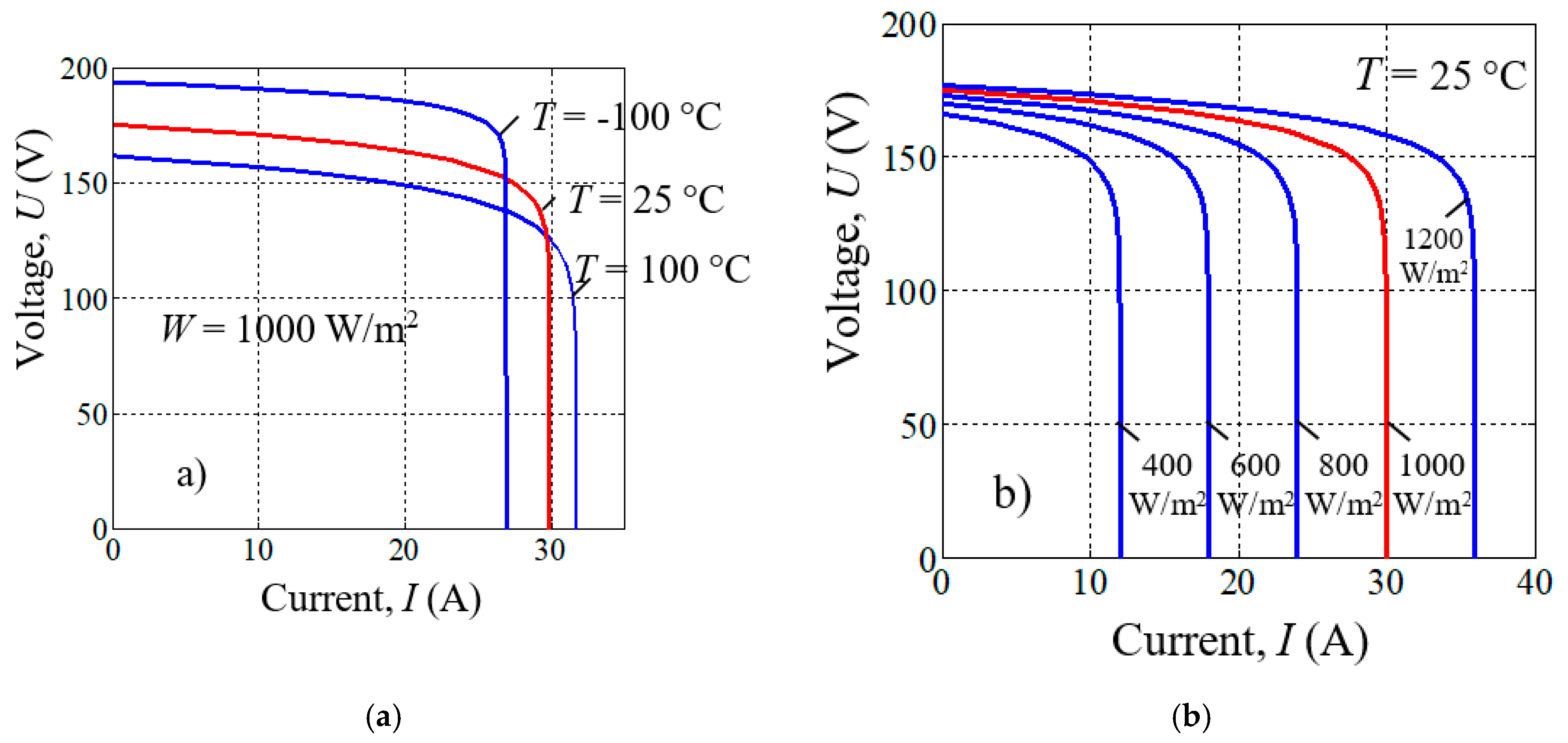
The resulting current–voltage characteristics are shown in
Figure 4.
The correspondence of the calculated characteristics obtained to their theoretical form indicates the adequacy of the Model (2)–(7). In addition, the resulting model is suitable for studying the operating modes of a solar panel when some of its cells are shaded and the temperature changes [
16,
17].
At nominal temperature Tn = 298 K and illumination Wn = 1000 W/m2, the panel delivers maximum power at I = 28 A and U = 150 V.
3.3. Study of the Dynamic Characteristics of a Solar Panel
3.3.1. Frequency Characteristics
The frequency characteristic of the solar panel is the dependence of its total complex output impedance on the frequency z(jω).
For the solar panel, the model of which is shown in
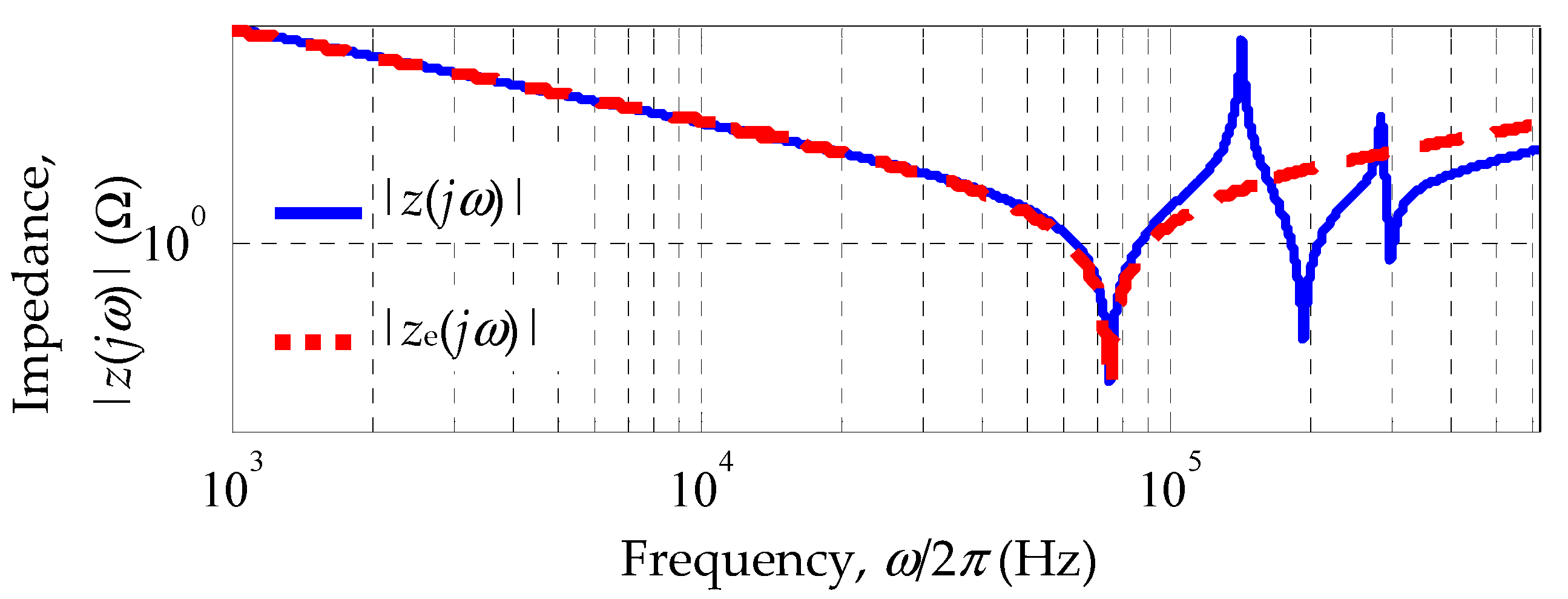
Figure 3, the amplitude and phase frequency characteristics are obtained, shown in
Figure 5.
In
Figure 5, one can see the frequencies at which the voltage resonance occurs: 75 kHz, 190 kHz and 300 kHz. At these frequencies, the solar panel impedance takes on a minimum value of 0.033 Ω; 0.1 Ω and 0.6 Ω, respectively. In the frequency range below the resonance frequencies, the solar panel impedance is capacitive, and the above-mentioned frequencies are inductive. The resulting phase shifts between the current supplied by the solar panel and the voltage at its terminals (in the lower frequency band, for example, the current leads the voltage) will have a significant effect on the dynamic characteristics of the control system.
Since the expected bandwidth of the control system does not exceed one thousand hertz and is significantly less than the first resonance frequency, then for those cases when a preliminary analysis of the system is carried out, an equivalent solar panel model can be drawn up, taking into account only one resonance with a frequency of 75 kHz, i.e., ωr = 2π × 75000 s−1. To do this, it is enough to use a circuit with a serial circuit ReLeCe, for which it is required to find the values of the equivalent elements Re, Le, and Ce.
The total complex impedance of the equivalent circuit is:
Since the following equality is valid at the resonance frequency of voltages:
then from (8) we obtain
, or
Re = 0.033 Ω (see
Figure 5).
To calculate
Le and
Ce, we will use Equation (9) and the condition of equality of the resistance of the original and equivalent circuits at a certain control frequency, for example,
ωk = 2π × 2000 s
−1. The value |
z(
jωk)| = 99 Ohms we get from
Figure 5.
Then the system of equations for determining
Le and
Ce takes the form:
Solution of (10):
Ce = 0.8 × 10
−6 F;
Le = 5.6 × 10
−6 H. The corresponding solar panel equivalent circuit is shown in
Figure 6.
The frequency response of the equivalent circuit is shown in
Figure 7, which coincides with the characteristics of the full equivalent circuit in the frequency range of the first resonance (see
Figure 5).
The presence of a fairly simple equivalent circuit makes it possible to analyze dynamic processes in a solar panel on a lumped model.
3.3.2. Analysis of the Joint Operation of a Solar Panel with a Shunt Switch
The solar panel and the shunt switch are connected by a cable, forming a closed loop that contains
R,
L, and
C elements connected in series (see
Section 3.3.1).
The presence of a closed loop with reactive elements leads to the fact that when the solar panel operates with a shunt switch, which switches at the frequency
fPM of the pulse-width modulator, fluctuations in currents and voltages will occur in the loop. These fluctuations will manifest themselves in the form of voltage ripples both at the output terminals of the solar panel and on its cells [
18,
19]. These phenomena are undesirable not only for consumers of constant voltage
UL = 120 V, but also for photocells of a solar panel, the nominal operating mode of which does not provide for the occurrence of reverse polarity voltage on them.
Let us conduct a quantitative study of these phenomena.
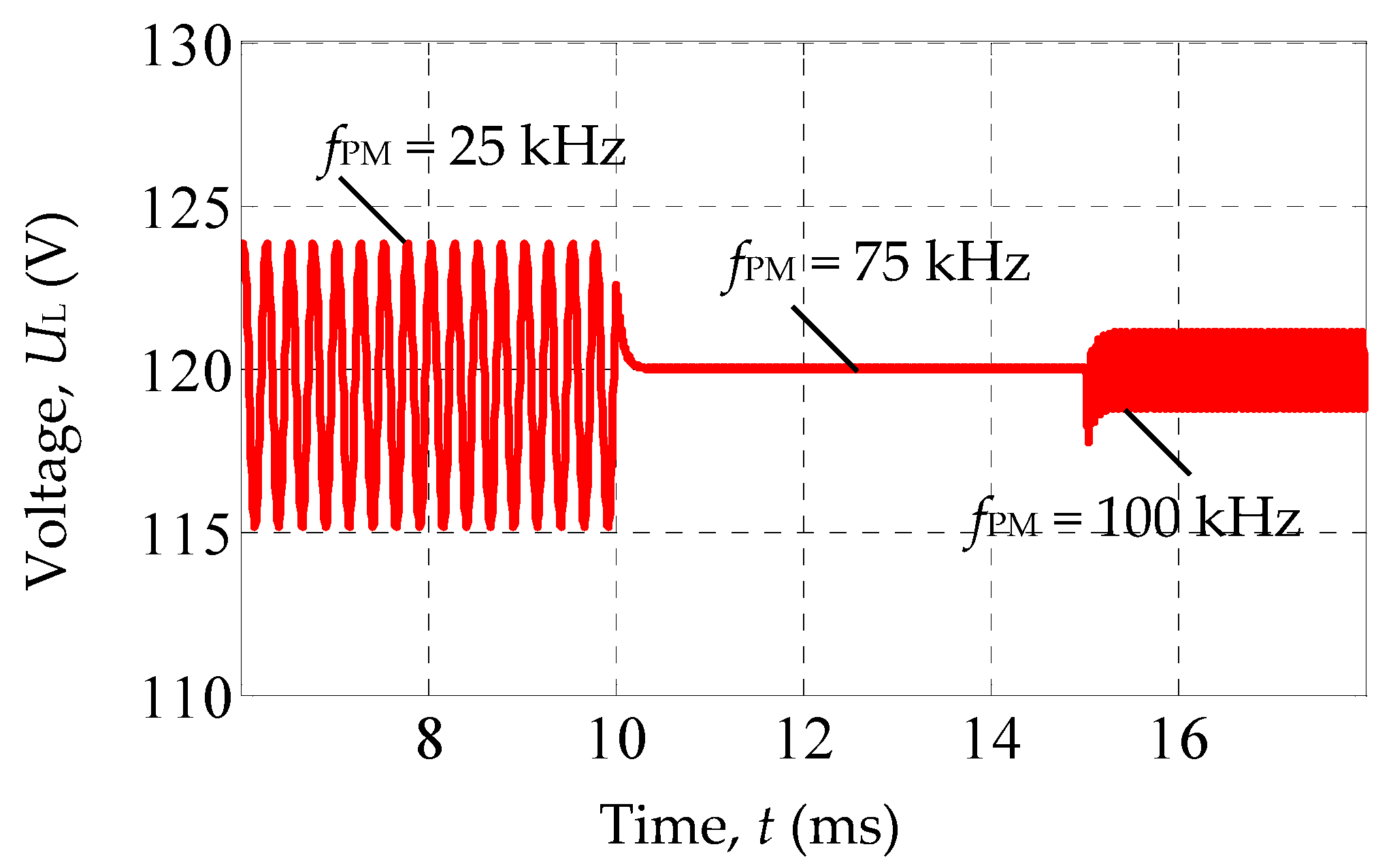
To determine the voltage ripple on the solar panel at different frequencies of current change, consider the mode of its operation with an active load
IL = 29 A, containing a harmonic component with a frequency
fPM and an amplitude of 0.1 A. This mode corresponds to the operating point on the steeply dipping section of the current–voltage characteristic of the solar panel, where the panel voltage is most sensitive to changes in current (see
Figure 4). The simulation results are shown in
Figure 8.
Ripple ∆ULof voltage UL at frequencies fPM = 25 kHz, 75 kHz, and 100 kHz were, respectively, ∆UL= ±4 V, ±0.015 V, and ±1.25 V. The ripple values at the voltage resonance frequency fr = 75 kHz are, as expected, negligible. This circumstance indicates the advisability of choosing the carrier frequency fPM of the pulse-width modulator equal to the resonance frequency fr. This choice will reduce the requirements for smoothing filters in the power supply system. Note that the presence of inductance in the cable that connects the solar panel to the switch shifts the actual resonance frequency downward relative to the value fr = 75 kHz.
Let us now consider transients on the photocells of the panel, i.e., voltage change
Up during shunt switching. According to the equivalent circuit in
Figure 2, this voltage in the model can be observed directly across the capacitor
Cp.
To analyze the transient processes due to the inherent properties of the solar panel, the model shown in
Figure A2 was used. In order to fully consider the course of the transient process, the switching frequency of the switch is chosen rather low:
fPM = 1 kHz.
The complete transient timing diagrams are shown in
Figure A3. The enlarged fragments of the change in the current
ISB at the panel output and voltage
Up on the photocells are shown in
Figure 9.
The analysis of the transient process in
Figure 9 shows that the fundamental harmonic of the current oscillations has a frequency
fr = 75 kHz. There are also small oscillations with a frequency of 200 kHz. Thus, the resonance frequency
fr = 75 kHz plays a dominant role in the transient processes of the solar panel when it works together with the shunt switch.
When the shunt switch is closed, the capacitor
Cp with a full charge voltage (in this case, about 170 V) begins to discharge. The discharge process is accompanied by its significant oscillation (see
Figure 9). In this case, the voltage on the capacitor, and therefore on the photocells, has an alternating character and reaches a value of −110 V. Such significant reverse voltages on photocells may be unacceptable according to the technical conditions of their operation. It is desirable to find such operating modes of the solar panel, in which the voltage fluctuations on the photocells did not leave the region of positive values.
Let us study how the switching frequency fPM of the shunt switch affects the alternating voltage character. It should be expected that the maximum oscillation amplitude will be observed at the resonance frequency fr = 75 kHz, and will decrease as the switching frequency fPM increases due to the proportional increase in the inductance resistance Lc.
For this study, the active resistance and inductance Lb,k of the cable connecting the solar panel with the shunt switch were introduced into the model.
Note that the introduction of the cable inductance
Lb,k = 4.8 × 10
−6 H between the panel and the switch reduces the frequency
fr of the panel resonance:
Simulation results for a range of frequencies
fPM = 25-55-88-110 kHz are shown in
Figure 10.
It follows from
Figure 10 that the full placement of the voltage fluctuation range
Up in the positive region occurs at a switching frequency
fPM not less than twice the resonant frequency of the solar panel, taking into account the cable connected to it. In this case, it is enough to choose
fPM = 110 kHz. We will use this value in the following calculations.
In general, the ratio fPM ≥ 2fp can be ensured not only by increasing the switching frequency fPM of the shunt switch, but also by reducing the resonant frequency fp by introducing, for example, an additional choke into the cable between the panel and the switch.
The need to fulfill the relation
fPM ≥ 2
fp leads to an increase in voltage ripple
V at the output terminals of the panel (see
Figure 8 and comments to it). Therefore, the decision to choose
fPM = 110 kHz requires the introduction of a low-pass filter into the power supply system. Its parameters are shown in
Figure A4.
4. System Controller Synthesis Method
As a result of the above study of the frequency responses of the system elements, it is advisable to design the controller based on the frequency responses of the open-loop system [
7,
20].
A simulation model for removing these characteristics is shown in
Figure A4, and the results of their construction are shown in
Figure 11:
Li,
φi are the initial and
Ld,
φd are the desired frequency response (decibel-log frequency response and phase-log frequency response).
Analysis of frequency responses indicates a significant phase stability margin: 90 degrees.
From
Figure 11, for the operating frequency range from 0 to 2000 Hz, the transfer functions of the initial
Wi(
s) and the desired
Wd(
s) open system are obtained:
From (11), we obtain an expression for the controller transfer function:
Transfer function (13) is a typical link of the isodrome [
21,
22].
The resulting link, or the so-called PI-regulator, is widely used in automatic control systems due to the following advantages [
23,
24]:
allows the possibility of synthesis based on a simplified Model (11) of the object;
the controller provides a zero steady-state error ε(t→∞) = 0 for constant action, i.e., first-order astatism not only with respect to the reference signal Ur, but also with respect to the disturbance—the load current IL(t);
provides a monotonic transient process in the system;
easy to implement in both continuous and discrete versions. In particular, most modern controllers support functions of PI regulation and pulse-width modulation signal shaping.
In addition, the introduction of a PI-regulator into the system requires checking the margin of its stability when the parameters of the object change. For this purpose, we will use the complete model of the synthesized system shown in
Section 5 and compose the differential equation of the system in small deviations with respect to the reference action
Ur(
t):
The nominal numerical values of the coefficients of Equation (14) are given in
Table A1.
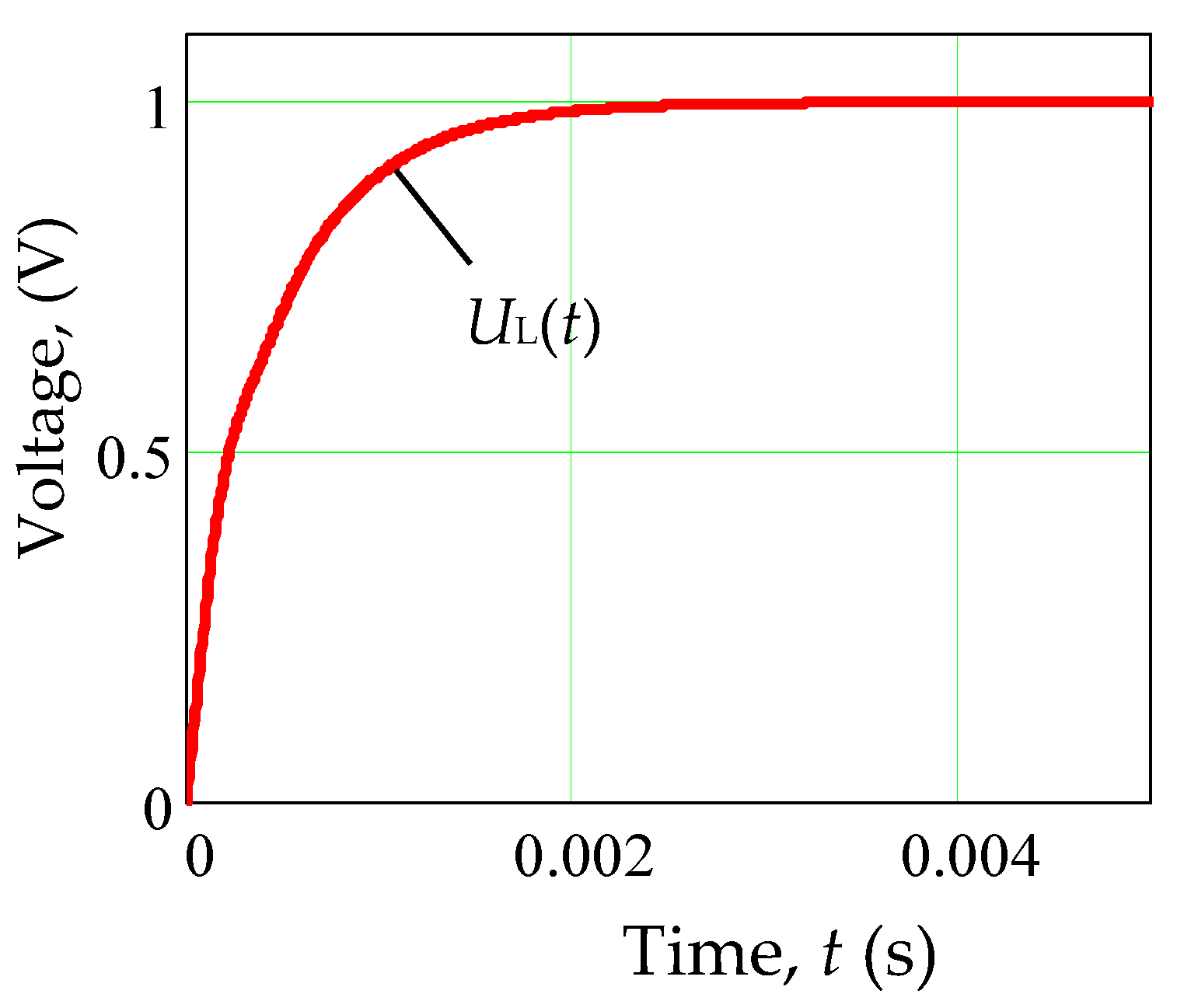
The transient process obtained from the differential Equation (14) for the voltage
UL(
t) with a single step jump of the reference signal
Ur(
t) is shown in
Figure 12 and has a monotonic character.
The transient time is about 2 ms (see
Figure 12). This characteristic of the system implies the most important requirement for the controller: the cycle time of its operation in the control loop should not exceed 0.2 ms.
To analyze the robustness of the system to change its parameters, let us first calculate its zeros and poles,
Table 2.
Analysis of
Table 2 allows us to single out three dominant poles for further study
s4 = −7.57 × 10
3 + 1.28 × 10
4i;
s5 = −7.57 × 10
3 + 1.28 × 10
4i,
s6 = −2.09 × 10
3, the real part of which is several orders of magnitude larger than the other poles.
Then, representing the characteristic polynomial
P(
s) of the system in the zpk-form
P(
s) = (
s −
s4)·(
s −
s5)·(
s −
s6), we obtain the characteristic equation:
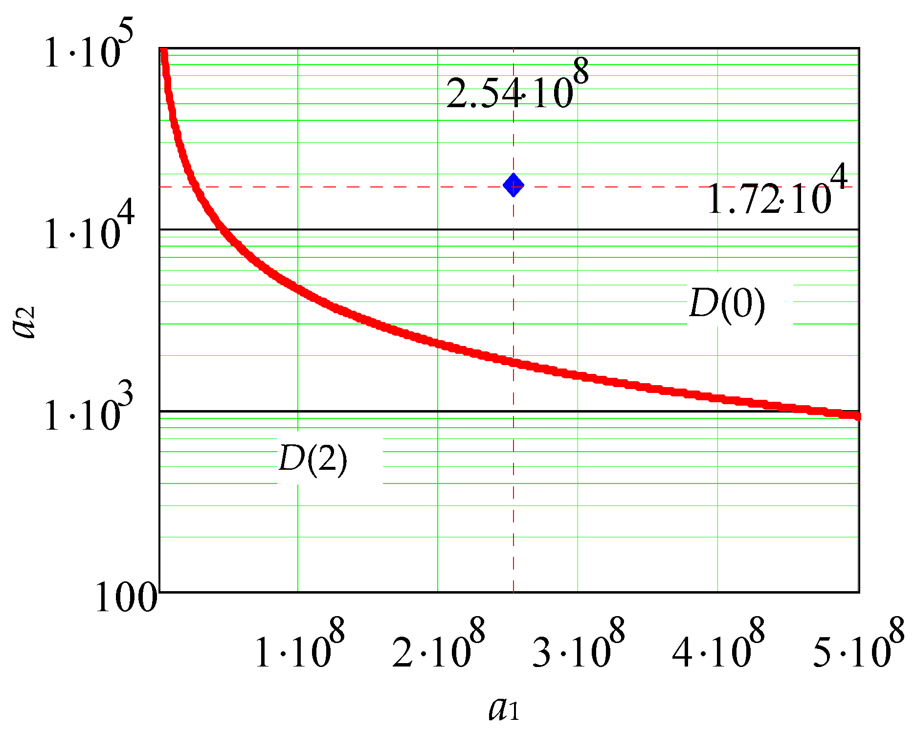
Rewriting (15) in the form:
and using the Hurwitz stability criterion:
a2a1 −
a0 > 0, we define the stability region
D(0) in the space of coefficients
a1,
a2 in the form of the inequality:
A graphical illustration of
D(0) is shown in
Figure 13. The nominal values
a1 and
a2 correspond to the operating point in the region
D(0), which is distant from the boundary of the stability region with approximately a 10-fold margin.
Let us proceed to the analysis of the robustness of the system to change the parameter a0.
The coefficient
a0 physically represents the transmission coefficient
k of an open-loop system, and to analyze its influence on the stability of the system, we construct a root locus for the range
k = (100…465…3000) × 10
9,
Figure 14.
When the transmission coefficient k of an open-loop system changes 30 times, the PI-regulator ensures that its stability is maintained, i.e., provides robust system stabilization.
5. Development of a General Control Algorithm
The design of the regulator, set out in
Section 4, provided for the control of one autonomous solar panel. However, as a rule, a large number of parallel solar panels are used in the power supply system of spacecraft [
4,
5].
The problem arises of finding a technical solution that will allow using the regulator calculated above to control solar array of any total power [
25,
26].
The trivial way to control one regulator simultaneously with all parallel solar panels has the following disadvantages:
upon disconnection or failure of a part of simultaneously controlled solar panels, the dynamic characteristics of the system change. This can lead not only to a deterioration in the quality of regulation, but also to a loss of system stability;
the shunt switches of all regulated solar panels are in switching mode. With a large number of switches, the total energy losses on the keys and their heating become significant. The size of devices for heat removal grows. As a result, the weight and size characteristics of the system deteriorate, and the probability of a failure in it increases.
To eliminate these disadvantages, it is proposed to form a solar array control algorithm based on homeostatic principles of multilevel and selectivity [
27,
28,
29,
30,
31].
The essence of these principles is that if the operating conditions of the system change to such an extent that it will not be able to maintain the normal performance of its functions, then there is a transition to another level of management, which has more resources to counter external influences [
32,
33].
In this case, the implementation of this control method consists in the fact that at load currents IL< 30 A, power supply is provided by only one solar panel with the conditional number 1. The rest of the solar panels are shunted by their switches, which are completely open, i.e., do not switch. If the load current becomes more than 30 A, i.e., the power of solar panel No. 1 will be completely exhausted, and then solar panel No. 2 will automatically connect. Now solar panel No. 1 (its switch is completely closed) gives its maximum current to the load, and the switch of solar panel No. 2 switches and maintains the set voltage level with small changes in the load current. The switches of all the remaining solar panel are still open, i.e., these solar cells do not participate in the power supply. As a result, only one solar panel is always in active regulation mode. At any load current, not the entire total power of the solar array supplied to the load is regulated, but only that part of it that falls on one solar panel. This ensures the constancy of the dynamic properties of the system and the high reliability of the shunt switches.
For automatic transfer of control between the solar panels, the general zone of regulation by shunt switches is divided into ranges, each of which determines the working area of only one solar panel,
Figure 15.
With a signal at the output of the regulator
Uc > 3.5 V, both solar panels tend to supply their full current to the power supply system. In the event that the sum of these currents (60 A) is excessive for consumers, and the inequality
Ur(
t) <
US(
t) begins to hold, then the error
ε(
t) =
Ur(
t) −
US(
t) becomes negative and, accordingly, the signal
Uc decreases. In this case, solar panel No. 2 will hit the active section
Uc = [2.5;3.5] V, within which the current delivered by it will be less than 30 A (see
Figure 15). If the total current of the solar array is still higher than the required one, then the voltage
Uc will continue to decrease, completely disconnect the solar panel No. 2, and go to the active section of the solar panel No. 1
Uc = [1;2] V, which will hold at the load currents
IL < 30 A.
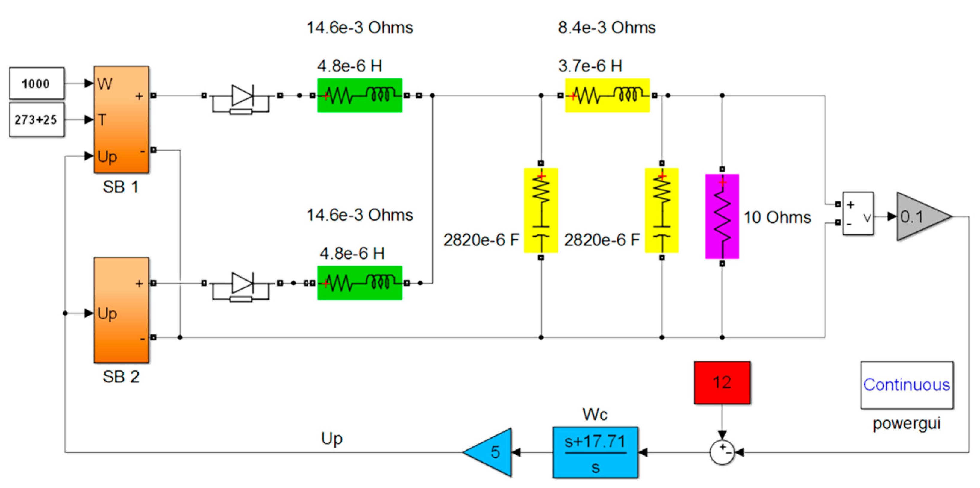
The structural diagram of the simulation model of the complete control system is shown in
Figure 16.
Blocks SB1 and SB2 include solar array models with actuators. Their contents are shown in
Figure A5.
6. Checking the System Quality Indicators on the Simulation Model
The quality indicators of the synthesized system were checked using the simulation model shown in
Figure 16. The system contains two solar panels, the current of each of which is limited to a maximum value of 30 A (at illumination
W = 1000 W/m
2 and temperature
T = 25 °C).
The main function of the control system is to maintain the load voltage at a constant level UL = 120 V with an allowable 5% deviation of this value in the current range IL = [0;50] A. In addition, the system must provide automatic connection or disconnection of the required amount of solar panels with variable shading and temperature changes in the range T = [−110;80] °C.
In accordance with these requirements, the system’s reactions to changes in the following values were studied:
load current when connecting and disconnecting consumers;
luminous flux density with partial shading of solar array;
solar panel temperature when the spacecraft enters and exits the shadow.
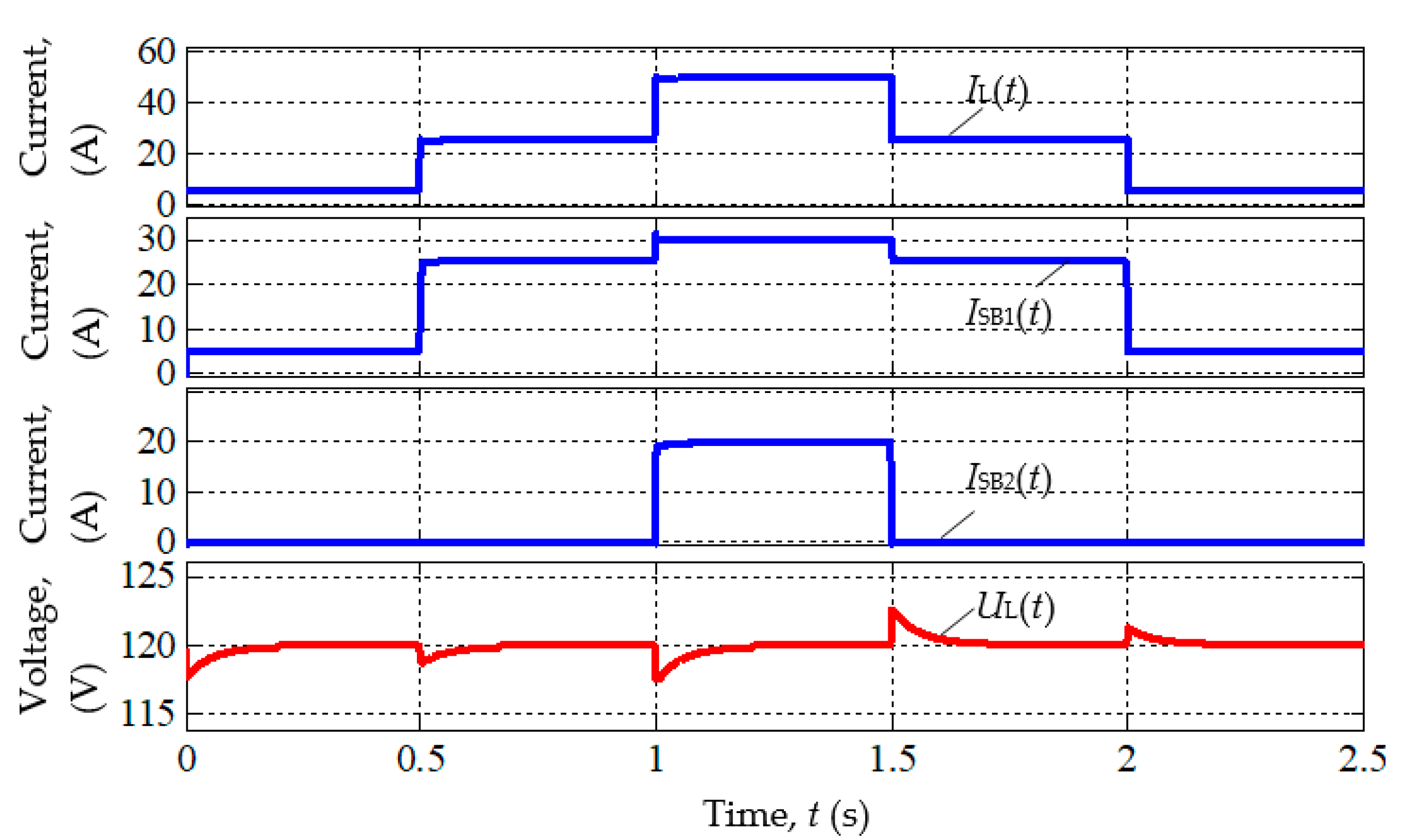
Figure 17 shows the response of the system to step changes in load current.
At time intervals t < 1 s and t > 1.5 s, the load current varies in the range from 5 to 25 A. Such values of currents can be supplied to the load by solar panel No. 1. Solar panel No. 2 is not connected to consumers, and voltage regulation is carried out only by the shunt switch of solar panel No. 1.
When the total consumer current increases to 50 A (t = [1;1.5] s), the control is automatically transferred to the second solar panel. In this case, the first solar panel delivers its full current of 30 A, and the second solar panel delivers a current of 20 A.
For all switchings, the surges of load voltage UL do not go beyond the 5% zone from 120 V: [114;126] V.
Figure 18 shows the transient processes in the system when the illumination of the first solar panel changes in the range
W = [200;1000] W/m
2 while maintaining the full illumination
W = 1000 W/m
2 of the second solar panel, i.e., partial shading mode is reproduced.
At illumination W = 1000 W/m2, the first solar panel delivers 25 A and fully supplies consumers. When its illumination is reduced to a value of W = 200 W/m2, the first solar panel can give consumers only 5 A, and the missing 20 A is delivered by solar panel No. 2. After restoring full illumination of the first solar panel, the second solar panel is automatically disconnected from the consumers, and control is again transferred to the active solar cell No. 1.
The ripple of load voltage UL is still within acceptable limits in this study.
Figure 19 reproduces the processes in the system when the temperature of the photocells of the first solar panel changes.
Analysis of
Figure 19 confirms the automatic transfer of control between the solar panels. At low temperatures, the first solar panel cannot provide the full current
IL = 29 A, and the load is distributed across two solar panels,
ISB1 ≈ 27 A,
ISB2 ≈ 2 A.
Thus, an experimental check confirms the system’s performance in a wide range of changes in external disturbing influences.
7. Discussion of the Results
Let us evaluate the compliance of the paper results with the goals stated in the introduction.
The mathematical model of the solar panel proposed in the paper has confirmed its adequacy and made it possible to carry out the planned studies of the control system on its basis. The model reveals the parametric dependence of the current–voltage characteristics of the solar panel on the luminous flux density and the temperature of the photocells. This made it possible to carry out a quantitative analysis of the operation of the control system in a given range of variation of the indicated values as disturbing influences.
The most important result of applying the proposed model is to obtain the dynamic characteristics of a solar panel in the frequency domain. The resonant properties of the solar panel, discovered as a result of the study of these characteristics, made it possible to establish the occurrence of a voltage of reverse polarity on its photocells, which is inadmissible according to the technical operating conditions. This phenomenon is eliminated by choosing the quantization frequency of the pulse-width modulator, at least twice the frequency of the lower resonance of the solar panel voltages together with the cable that connects it to the shunt switch.
The choice of the quantization frequency in accordance with this recommendation made it possible to ensure the quasi-continuity of the system in the operating frequency band and, as a consequence, to carry out a simple graphic-analytical identification of its parameters in the form of a dynamic first-order link. Implemented on this basis, the algebraic method for the synthesis of the controller ended in obtaining an analytical model of the controller in the form of a proportional-integral link. The introduction of this link into the control loop turned out to be sufficient to form the desired static and dynamic characteristics of the system, and the inclusion of an additional corrective link in it was not required.
For power supply systems using a large number of solar panels, a general control algorithm is proposed that reproduces the homeostatic mechanism of the functioning of biological systems. For this purpose, a multi-level, hierarchical structure of information and energy interaction of solar panels is formed in the system, which ensures the transfer of control from a lower level to a higher level only if the energy resources of the lower level are exhausted. The modular structure of such a structure, combined with its multilevel structure, allows one at any time to actively control not all the power supplied to consumers, but only that part of it that corresponds to the power of one module. This eliminates the occurrence of a cascading, increasing propagation of failures in the system, since any single failure is localized in one module, and the functions of the faulty module are redistributed between the remaining solar panels. The described mechanism of homeostasis gives the power supply system the property of survivability, which is necessary in spacecraft intended for long-term autonomous flights.
The verification of the specified approach to organizing the joint operation of several solar panels, carried out in the paper, demonstrated high flexibility and efficiency of transferring control between them. It should be noted that the proposed algorithm for solar array control corresponds to the modern concept of building cyber-physical systems.
8. Conclusions and Prospects for Further Studies
Let us briefly formulate the results of the work.
General scientific result:
The proposed modular principle of constructing a control system with the organization of a hierarchical structure of interaction of solar panels makes it possible to reproduce the homeostatic mechanism of functioning of biological organisms in the power supply system. The implementation of this mechanism provides the power supply system with the vitality property required in spacecrafts intended for long-term autonomous flights.
Applied results:
The developed mathematical model of the solar panel and the studies carried out using this model made it possible to establish that when the panel works together with a shunt PWM switch, a voltage resonance occurs in it. In this case, a voltage of reverse polarity appears on the photocells, which is unacceptable according to the technical conditions of their operation.
To eliminate the voltage of reverse polarity, it is recommended to use a PWM signal with a sampling frequency of at least twice the lower resonance frequency of the solar panel with a switch. The simulation results confirmed the effectiveness of this recommendation.
Frequency analysis of the characteristics of the power supply system indicates the possibility of achieving the control goal with the PI controller. The use of this controller provides a monotonic nature of transient processes in the system and zero steady-state control error in the presence of disturbing influences: changes in load current, illumination, and temperature of solar photocells.
Root analysis of the differential equation of the control system confirms the high degree of its robustness in relation to changes in internal parameters and external load parameters.
Prospects for further studies:
- ○
Providing consumers with electric energy in conditions of complete shading of solar panels requires the presence of storage batteries on the spacecraft. In this regard, an urgent task for further studies is to analyze the joint work and transfer of control between the control subsystems of solar arrays and storage batteries.
- ○
Concentration of electrical equipment in spacecrafts sets the task of electromagnetic compatibility of this equipment, including the task of ensuring the noise immunity of the power supply system itself. The relevance of this problem increases when spacecraft leave the near-earth space and during flights under conditions of the full spectrum of cosmic radiation.
- ○
The current trend of increasing the service life of space equipment up to 15 years and more brings to the fore the problem of the robustness of the operational characteristics of this equipment to the inevitable change in the parameters of the internal elements. Ensuring this robustness presupposes a transition from the simplest principle of output control to state control; in particular, to modal control. The study of the possibilities of modal control for maintaining the quality of regulation in a wide range of system parameters is also of practical and scientific interest for further studies.


