Corrected Evolutive Kendall’s τ Coefficients for Incomplete Rankings with Ties: Application to Case of Spotify Lists

Abstract

Mathematical analysis of rankings is essential for a wide range of scientific, public, and industrial applications (e.g., group decision-making, organizational methods, R&D sponsorship, recommender systems, voter systems, sports competitions, grant proposals rankings, web searchers, Internet streaming-on-demand media providers, etc.). Recently, some methods for incomplete aggregate rankings (rankings in which not all the elements are ranked) with ties, based on the classic Kendall’s tau coefficient, have been presented. We are interested in ordinal rankings (that is, we can order the elements to be the first, the second, etc.) allowing ties between the elements (e.g., two elements may be in the first position). We extend a previous coefficient for comparing a series of complete rankings with ties to two new coefficients for comparing a series of incomplete rankings with ties. We make use of the newest definitions of Kendall’s tau extensions. We also offer a theoretical result to interpret these coefficients in terms of the type of interactions that the elements of two consecutive rankings may show (e.g., they preserve their positions, cross their positions, and they are tied in one ranking but untied in the other ranking, etc.). We give some small examples to illustrate all the newly presented parameters and coefficients. We also apply our coefficients to compare some series of Spotify charts, both Top 200 and Viral 50, showing the applicability and utility of the proposed measures.

1. Introduction

The analysis of rankings of scores (cardinal rankings) or, particularly, rankings composed of natural numbers (ordinal rankings), have been studied from different perspectives attending to the ultimate goal of the researchers or practitioners (see [1]). When the interest is on obtaining a consensus score that summarizes the opinion of various judges, the used mathematical tools are usually aimed to find a ranking that minimizes a given distance metric (see the seminal paper [2,3] for some properties of different metrics). In such a case, we say that a distance metric minimizes disagreement. We can place in this area the methods called voter systems, ranking aggregation, and others (see the detailed review in [4]).

When the interest is focused on comparing two series of rankings, one of the key points is to obtain a measure that describes the evolution of the series. In this case, we have a series of rankings such that each one of them prioritizes the elements based on the scores obtained at a particular time (see [5]). For example, sports rankings belong to this category. Obviously, at the end of a season, there is no need to find a consensus ranking since, by the nature of sports leagues, it is the last ranking that serves to summarize the result of the overall season. The same happens with the Stock Market, the richest people rankings made by the Fortune magazine [6], university rankings (e.g., [7,8]), songs rankings based on the number of downloads, streaming, or sales (see [9]), etc. Our work is focused on a series of rankings behavior.

The terminology applied to rankings is not unique. For example, in [10] the term partial is used to indicate rankings in which ties are presented, while in [11] the term partial indicates that not all the objects are compared. In this paper, we use the terminology coined in [4,12]. We talk of complete rankings when all the objects are compared (as in a football league) and incomplete when there are absent objects (as in a Top k ranking). We explicitly use the terms with ties or without ties to indicate whether we consider the presence of tied objects in the rankings. We recall that in [11] the term linear order is used when all objects are compared and no ties are allowed (that is, for us, complete rankings with no ties) and the term weak ordering when all objects are compared, but ties are allowed (that is, for us, complete rankings with ties).

Incomplete rankings appear in multiple areas. For example, in national or European grant calls, judges evaluate only a subset of the applications, and therefore each judge handles an incomplete ranking. The same happens in literary contests, where each judge only reads a small number of manuscripts. In the case of the results shown by search engines, it is clear that only the first Top k web pages are displayed, being, as a consequence, an incomplete ranking.

We use, and extend, the results of some previous papers. Some concepts are taken from [5], where a method to compare series of complete rankings with no ties was presented, and from [13], where a method to compare series of complete rankings with ties was analyzed. We also make reference to [14], where some theoretical aspects where studied. In all these works, there are two main ingredients:

1.

The use of generalizations of the classical concept of Kendall’s $\tau$ coefficient of disagreement [15,16,17];

2.

The use of graphs associated to the series of rankings as a tool to visualize and also to help in the definition the coefficients that summarize the “behaviour” of the series of rankings.

Regarding to extensions of Kendall’s $\tau$ coefficient, the first attempt to incorporate an axiomatic distance metric was in [2], followed by the works [11,18,19].

More recently, in [4] these previous works were revised and a new axiomatic framework for incomplete rankings was introduced. To the best of our knowledge, the last paper devoted to an axiomatic study for incomplete rankings is [12], where it is shown as an extension of Kendall’s $\tau$ coefficient to the case of incomplete rankings with ties.

Kendall’s $\tau$ has been extensively used, and some extensions can be found in the literature up to the present day on [10,12,20]. In particular, Kendall’s $\tau$ has been recently reviewed for ophthalmic research in [21] and it is a tool used in neuroscience studies—e.g., [22]—and in bioinformatics [23].

Regarding the use of graphs to represent a series of rankings, we recall, in particular, that a graph can be used to describe the crossings between two rankings. This graph is called a permutation graph (see [24,25]). When a graph is defined to show the consecutive crossings between a series of m rankings, it is called a Competitivity graph [5]. This concept corresponds to that of intersection graph of a concatenation of permutation diagrams in graph theory (see [26]). For more relations on graphs associated with rankings, see [14].

In this paper, we take some results of [4,12] as our starting point to develop two coefficients to describe the evolution of a series of $m\ge 2$ incomplete rankings with ties. When applied to the case of only two rankings, our measures reduce to the measures given in [4,12].

We also extend the study of a series of complete rankings with ties developed in [13] to the case of incomplete rankings with ties. We make use of the standard modern notation in the field of rankings mainly based on [10,12,27], among others.

We take as our starting point the definition of ${\tau }_x$ of [12] that is based on the computation of a certain sum of the form ${\sum }_{i=1}^n{\sum }_{j=1}^n{A}_{ij}{B}_{ij}$ that involves the terms of some matrix A and B that indicate the relative positions of the elements of two rankings. In Theorem 1, we give an expression of this sum as a function of the type of interactions between a pair of elements $\{i,j\}$ from one ranking to the next one (e.g., interchanges from tie to untie, absence of one of the elements in one ranking, crossings, etc.). This result allows for writing ${\tau }_x$ (and ${\widehat{\tau }}_x$) in terms of the interactions of the elements of the rankings.

On the one hand, this theoretical result also allows a computation of the sum ${\sum }_{i=1}^n{\sum }_{j=1}^n{A}_{ij}{B}_{ij}$ without computing explicitly the involved matrices. On the other hand, it allows for interpreting the interactions of a series of rankings by using a permutation graph or, more generally speaking, a competitivity graph. The edges are weighted to represent the weight of the corresponding interactions and the whole series of rankings.

We define two coefficients ${\tau }_{ev}^{•}$ and ${\widehat{\tau }}_{ev}^{•}$ for series of incomplete rankings with ties by using an analogy based on previous well-established definitions. We recall that, in the field of incomplete rankings, “intuition” is usually used for some measures over others since when you handle an incomplete ranking, there is no unique form to interpret the results (see this kind of reasoning in [4,12]). In our case, our measures’ behaviour is checked by ensuring that they are well normalized and that they reduce to well-known cases in limit situations.

Finally, other contributions of the paper are placed on a practical field. We give a methodology to study the movements of rankings (of songs) in Spotify by using two different approaches: the cases of series of incomplete rankings without ties and series of incomplete rankings with ties.

The structure of the paper is as follows. In Section 2, we recall Kendall’s $\tau$ and give the fundamental relations that will be useful throughout the paper. In Section 3, we recall the notation and basic results for the case of two incomplete rankings with ties allowed.

In Section 4, we give the fundamental theoretical result of the paper and some remarks that give insight both into the validity and application of this result. In Section 5, we recall some definitions from [13] to measure the evolution of m complete rankings with ties. In Section 6, we present two coefficients, denoted as ${\tau }_{ev}^{•}$ and ${\widehat{\tau }}_{ev}^{•}$ to characterize the evolution of m incomplete rankings with ties and some examples are given. In Section 7, we illustrate the applicability of the new coefficients by using some real data obtained from Spotify charts. Finally, in Section 8, we outline the main conclusions of the paper.

2. Preliminaries

In [16] it is shown that Kendall’s $\tau$ coefficient (also called measure of disarray) associated with two rankings with the same number of elements n, can be written in the form

$$\tau =1-\frac{2s}{\frac{1}{2}n(n-1)}$$

(1)

where s is the minimum number of interchanges required to transform one ranking into the other. This coefficient is a measure of the intensity of rank correlation. The coefficient can also be written as

$$\tau =\frac{P-Q}{\frac{1}{2}n(n-1)}$$

(2)

where P is the number of pair of elements that maintain its relative order when passing from the first ranking to the second one (that is, the first element is above or below the second in both rankings) and Q is the number of pairs of elements that interchange its order (that is, in one ranking, the first element is above the second and, in the other ranking, the first element is below the second, or vice-versa).

Note that Q and s are equal. Furthermore, this quantity can be identified with the number of crossings or inversions when passing from the first ranking to the second. For this reason, throughout the paper, we will keep in mind that Equation (1) gives the equivalence between the number of crossings and the associated $\tau$. This will be important in what follows since we will deal with different extensions of Kendall’s $\tau$ coefficient and since one of our preferred tools will be counting the number of crossings, as in [5].

We recall from [27] that a distance metric $d(\mathbf{a},\mathbf{b})$ can be transformed into a correlation coefficient $\tau (\mathbf{a},\mathbf{b})$ by the formula

$$\tau (\mathbf{a},\mathbf{b})=1-\frac{2d(\mathbf{a},\mathbf{b})}{d_{max}(\mathbf{a},\mathbf{b})}$$

(3)

where $d_{max}(\mathbf{a},\mathbf{b})$ is the maximum possible distance between two rankings. We recall that a distance metric between two rankings $\mathbf{a}$ and $\mathbf{b}$ is a non-negative real function f, such that it is symmetric ($f(\mathbf{a},\mathbf{b})=f(\mathbf{b},\mathbf{a})$, for any pair of rankings), regular ($f(\mathbf{a},\mathbf{b})=0\leftrightarrow \mathbf{a}=\mathbf{b}$) and satisfying the triangle inequality ($f(\mathbf{a},\mathbf{c})\le f(\mathbf{a},\mathbf{b})+f(\mathbf{b},\mathbf{c})$, for any rankings a, b, and c). Note that Equation (1) is of this form, since $n(n-1)/2$ is the maximum number of crossings between two given rankings. The same happens with the Spearman’s $\rho$ coefficient. In [16] the Spearman’s $\rho$ for two ordinal complete rankings $\mathbf{x}=(x_1,x_2,\dots ,x_n)$ and $\mathbf{y}=(y_1,y_2,\dots ,y_n)$ with $x_i,y_i\in \mathbb{N}$ is defined by

$$\rho =1-\frac{6{\sum }_{i=1}^n{(x_i-y_i)}^2}{n^3-n}$$

and this is of the form (3) since it is easy to show that the maximum value of ${\sum }_{i=1}^n{(x_i-y_i)}^2$ occurs when one ranking is the reverse of the other and, as a consequence, the maximum value of the distance metric $d(\mathbf{x},\mathbf{y})={\sum }_{i=1}^n{(x_i-y_i)}^2$ is $\frac{1}{3}(n^3-n)$ (see [3] for this and other properties of distance metrics).

We also recall that a permutation graph (called competitivity graph in [5]) is associated with two rankings over the same elements in such a way that the nodes represent the elements and two nodes and are connected with an edge if they cross their positions when passing from one ranking to the other.

In this way, it is clear that the number of edges of this graph is, precisely, s. Furthermore, another quantity (borrowed from graph theory) is also introduced in [5]: the Normalized Mean Strength $NS$; that is, the normalized sum of the weights of the edges of a weighted graph. When considering only two rankings and its corresponding competitivity graph, we have the following relation

$$NS=\frac{1-\tau }{2}$$

(4)

that gives the equivalence between the Normalized Mean Strength and Kendall’s $\tau$ for two rankings. Note that $\tau \in [-1,1]$ and $NS\in [0,1]$. We consider that the measure $NS$ is more intuitive than $\tau$ since it allows us to interpret the movements or activity of a series of rankings as a percentage.

3. Coefficients for Two Incomplete Rankings with Ties

In this section, we recall some definitions used in [4,12]. We will use the next three ingredients in order to define a coefficient to compare two rankings:

1.

A vector to define the ordinal ranking (including the description of absent elements and tied elements);

2.

A matrix to indicate the relative positions of the elements of the ranking (including absent and tied elements);

3.

A formula to define the coefficients for a pair of rankings by using the entries of their associate matrices defined in the previous step.

Let $V=\{v_1,v_2,\cdots ,v_n\}$ be the objects to be ranked, with $n>1$. The ranking is given by

$$\mathbf{a}=[a_1,a_2,\cdots ,a_n]$$

(5)

where $a_i$ is the position of $v_i$ in the ranking. Note that if $a_i=a_j$, then $v_i$ and $v_j$ are tied. If $v_i$ is not ranked, then it is denoted as $a_i=•$. We also define the set

$$V_{\mathbf{a}}=\{v_i\in V|a_i\ne •\}.$$

We define an $n\times n$ matrix $A=\left(A_{ij}\right)$, with entries $A_{ij}$ associated to $\mathbf{a}$ as follows:

$$A_{ij}=\left\{\begin{array}{cc}\hfill 1& \mathrm{if}{a}_i\le a_j\hfill \\ \hfill -1& \mathrm{if}{a}_i>a_j\hfill \\ \hfill 0& \mathrm{if}i=j,a_i=•,\mathtt{or}{a}_j=•\hfill \end{array}\right.$$

(6)

According to [12], we define the coefficients

$${\tau }_x(\mathbf{a},\mathbf{b})=\frac{{\sum }_{i=1}^n{\sum }_{j=1}^n{A}_{ij}{B}_{ij}}{n(n-1)}$$

(7)

and, when $\overline{n}>1$

$${\widehat{\tau }}_x(\mathbf{a},\mathbf{b})=\frac{n(n-1)}{\overline{n}(\overline{n}-1)}{\tau }_x(\mathbf{a},\mathbf{b})$$

(8)

where $\overline{n}$ is the number of common ranked elements $v_i$ to $\mathbf{a}$ and $\mathbf{b}$. That is:

$$\overline{n}=|V_a\cap V_b|$$

(9)

Example 1.

Let $V=\{1,2,3,4,5,6,7,8\}$, and let us consider two rankings $\mathbf{a}$ and $\mathbf{b}$. Then, $\mathbf{a}=[6,4,5,5,•,2,1,3]$ represents the incomplete ranking with ties $(7,6,8,2,3-4,1)$, where $3-4$ indicate tied elements. Analogously, $\mathbf{b}=[3,3,2,2,•,1,•,4]$ represents the ranking $(6,3-4,1-2,8)$. Note that $n=8$ and $\overline{n}=6$.

Note that ${\tau }_x$ with complete rankings and no ties reduces to the classic Kendall’s $\tau$ given by (1), while ${\widehat{\tau }}_x$ is a renormalization of ${\tau }_x$, verifying $|{\widehat{\tau }}_x|\ge |{\tau }_x|$.

As we will see, Definition 6 in Section 6, is based on an analogy with Equation (1). To that end, it will be necessary to count all the possible cases when passing from $\mathbf{a}$ to $\mathbf{b}$ (interactions between the relative positions of pair of elements such as crossings, pass from tie to untie, from being in the ranking to quitting it, etc.). We do this in the next section.

4. Main Result

The following result is the fundamental theoretical result of this paper. This result will allow us to write ${\tau }_x$ and ${\widehat{\tau }}_x$ in terms of the interactions of the rankings’ elements. It opens the possibility of giving weights to the interactions, as is a common practice in modern definitions of Kendall’s tau [10]. This result also constitutes our starting point to define a coefficient for a series of more than two incomplete rankings. This theorem also allows giving insight into the differences between ${\tau }_x$ and ${\widehat{\tau }}_x$. Some other consequences are detailed in the remarks below and in Corollary 1.

Theorem 1.

Given two vectors $\mathbf{a}$, $\mathbf{b}$ representing incomplete rankings of n elements with ties, represented as in (5), and their corresponding matrices $A=\left(A_{ij}\right)$ and $B=\left(B_{ij}\right)$ defined by (6), it holds that

$$\sum _{i=1}^n\sum _{j=1}^n{A}_{ij}{B}_{ij}=n(n-1)-4s-2n_{tu}-2N_{inc}$$

(10)

where

$$N_{inc}=\left(\genfrac{}{}{0pt}{}{n_{••}}{2}\right)+\left(\genfrac{}{}{0pt}{}{n_{\ast •}}{2}\right)+\left(\genfrac{}{}{0pt}{}{n_{•\ast }}{2}\right)+n_{••}(n_{\ast •}+n_{•\ast }+n_{\ast \ast })+n_{\ast \ast }(n_{\ast •}+n_{•\ast })+n_{\ast •}{n}_{•\ast }$$

(11)

• s is the number of crossings—that is, the number of pairs $\{i,j\}$—such that $a_i<a_j$ and $b_i>b_j$, or $a_i>a_j$ and $b_i<b_j$.
• $n_{tu}$ is the number of pairs that are tied in only one ranking (from tie to untie or viceversa), that is, such that $a_i=a_j$ and $b_i\ne b_j$, or $a_i\ne a_j$ and $b_i=b_j$.

In the definitions of s, and $n_{tu}$, it is assumed that $a_i$ and $b_i$ are different from •. For the cases when one or more • may appear, the following notation holds:

• $n_{••}$ is the number of entries such that $a_i=b_i=•$;
• $n_{•\ast }$ is the number of entries, such that $a_i=•$ and $b_i\ne •$;
• $n_{\ast •}$ is the number of entries, such that $a_i\ne •$ and $b_i=•$.

Finally, it is also needed to define $n_{\ast \ast }$ as the number of entries, such that $a_i\ne •$ and $b_i\ne •$.

Proof of Theorem 1. 

For each pair $\{i,j\}$ we will evaluate each term $A_{ij}{B}_{ij}+A_{ji}{B}_{ji}$ in the expression ${\sum }_{i=1}^n{\sum }_{j=1}^n{A}_{ij}{B}_{ij}$. The case $i=j$ gives $A_{ii}{B}_{ii}+A_{ii}{B}_{ii}=0$.

Thus, we focus on pairs $\{i,j\}$ with $i\ne j$. There is a total number of $n(n-1)/2$ of these pairs. It is useful to consider the basic cell of the pair $\{i,j\}$ with $i<j$.

$$\left(\begin{array}{cc}{a}_i& b_i\\ a_j& b_j\end{array}\right)$$

where $a_k$ and $b_k$ can be natural numbers or a • if the element k is not ranked in $\mathbf{a}$ or $\mathbf{b}$.

Let us study first the cases that can appear when no • is present in the basic cell.

The Complete Case (C):

That is $a_k\ne •,b_k\ne •$, for all $k\in \{1,2,\dots n\}$. We distinguish four types of basic cells.

Type C.1: Not crossing, and no ties in a nor in b.

For example:

$$\left(\begin{array}{cc}1& 3\\ 2& 4\end{array}\right)\mathrm{or}\left(\begin{array}{cc}2& 4\\ 1& 3\end{array}\right).$$

So that, we have $a_i\ne a_j$ and $b_i\ne b_j$ and two cases can appear:

C.1.1.

If $a_i<a_j\mathrm{and}{b}_i<b_j$, then $A_{ij}{B}_{ij}+A_{ji}{B}_{ji}=1·1+(-1)·(-1)=2$.

C.1.2.

If $a_i>a_j\mathrm{and}{b}_i>b_j$, then $A_{ij}{B}_{ij}+A_{ji}{B}_{ji}=(-1)·(-1)+1·1=2$.

Type C.2: Crossing.

For example:

$$\left(\begin{array}{cc}1& 4\\ 2& 3\end{array}\right)\mathrm{or}\left(\begin{array}{cc}2& 3\\ 1& 4\end{array}\right).$$

Again, we have $a_i\ne a_j$ and $b_i\ne b_j$ and two more cases can appear:

C.2.1.

If $a_i<a_j\mathrm{and}{b}_i>b_j$, then $A_{ij}{B}_{ij}+A_{ji}{B}_{ji}=1·(-1)+(-1)·1=-2$.

C.2.2.

If $a_i>a_j\mathrm{and}{b}_i<b_j$, then $A_{ij}{B}_{ij}+A_{ji}{B}_{ji}=(-1)·\left(1\right)+1·(-1)=-2$.

Type C.3: From tie to untie or viceversa.

For example:

$$\left(\begin{array}{cc}1& 3\\ 1& 4\end{array}\right),\left(\begin{array}{cc}1& 4\\ 1& 3\end{array}\right),\left(\begin{array}{cc}3& 1\\ 4& 1\end{array}\right),\mathrm{or}\left(\begin{array}{cc}4& 1\\ 3& 1\end{array}\right)$$

We have $a_i=a_j\mathrm{and}{b}_i\ne b_j$ or $a_i\ne a_j\mathrm{and}{b}_i=b_j$. Therefore, four cases can appear:

C.3.1.

If $a_i=a_j\mathrm{and}{b}_i<b_j$ then $A_{ij}{B}_{ij}+A_{ji}{B}_{ji}=1·1+1·(-1)=0$.

C.3.2.

If $a_i=a_j\mathrm{and}{b}_i>b_j$ then $A_{ij}{B}_{ij}+A_{ji}{B}_{ji}=1·(-1)+1·1=0$.

C.3.3.

If $a_i<a_j\mathrm{and}{b}_i=b_j$ then $A_{ij}{B}_{ij}+A_{ji}{B}_{ji}=1·1+(-1)·1=0$.

C.3.4.

If $a_i>a_j\mathrm{and}{b}_i=b_j$ then $A_{ij}{B}_{ij}+A_{ji}{B}_{ji}=(-1)·1+1·1=0$.

Type C.4: From tie to tie.

For example:

$$\left(\begin{array}{cc}1& 2\\ 1& 2\end{array}\right)$$

That is, we have: $a_i=a_j\mathrm{and}{b}_i=b_j$, and then $A_{ij}{B}_{ij}+A_{ji}{B}_{ji}=1·1+1·1=2$.

We denote the number of pairs of each case using the terminology of

Table 1. Number of pairs $\{i,j\}$ corresponding to each type for the complete cases.

Type	Number of Pairs
C.1	$n_{nc}$
C.2	s
C.3	$n_{tu}$
C.4	$n_{tt}$

. Note that $n_{tt}$ is the number of pairs that are tied in both rankings, that is, such that $a_i=a_j$ and $b_i=b_j$. Note also that $n_{tu}$ is the number of pairs that go from tie to untie or viceversa.

The Incomplete Case (I):

There is at least one • in the basic cell. In other words, there is some k such that $a_k=•$, or $b_k=•$, or both. We distinguish seven cases:

Type I.1: Four • That is $a_i=a_j=b_i=b_j=•$, or graphically

$$\left(\begin{array}{cc}•& •\\ •& •\end{array}\right)$$

Then $A_{ij}{B}_{ij}+A_{ji}{B}_{ji}=0·0+0·0=0$. Let us denote by $n_{••}$ the number of null rows that appear in the matrix with columns $\mathbf{a}$ and $\mathbf{b}$. Therefore, we have $\left(\genfrac{}{}{0pt}{}{n_{••}}{2}\right)$ pairs $\{i,j\}$ of this type.

Type I.2: Three •. That is, a cell of one of these forms

$$\left(\begin{array}{cc}•& •\\ \ast & •\end{array}\right),\left(\begin{array}{cc}\ast & •\\ •& •\end{array}\right),\left(\begin{array}{cc}•& •\\ •& \ast \end{array}\right),\mathrm{or}\left(\begin{array}{cc}•& \ast \\ •& •\end{array}\right)$$

where ∗ is a number (not a •). Therefore, we have four cases, but all are similar to this one: $a_i\ne •$ and $a_j=b_i=b_j=0$. Then, $A_{ij}{B}_{ij}+A_{ji}{B}_{ji}=0·0+0·0=0$.

Denoting $n_{\ast •}$ the number of rows of the form $(\ast •)$ in the $n\times 2$ matrix $\left(\mathbf{a}\mathbf{b}\right)$, and $n_{•\ast }$ the number of rows of the form $(•\ast )$ in the same matrix, it is clear that the number of pairs $\{i,j\}$ of this type is: $n_{••}(n_{\ast •}+n_{•\ast })$.

Type I.3: Two •, one on each ranking. That is, any cell of one of these forms

$$\left(\begin{array}{cc}•& •\\ \ast & \ast \end{array}\right),\left(\begin{array}{cc}\ast & \ast \\ •& •\end{array}\right),\left(\begin{array}{cc}•& \ast \\ \ast & •\end{array}\right),\mathrm{or}\left(\begin{array}{cc}\ast & •\\ •& \ast \end{array}\right)$$

These four cases can be reduced to two:

I.3.1.

If $a_i=b_i=•,a_i\ne •\mathrm{and}{b}_j\ne •$, then $A_{ij}{B}_{ij}+A_{ji}{B}_{ji}=0·0+0·0=0$.

I.3.2.

If $a_i=•,a_j\ne •,b_i\ne •\mathrm{and}{b}_j=•$, then $A_{ij}{B}_{ij}+A_{ji}{B}_{ji}=0·0+0·0=0$.

Denoting by $n_{\ast \ast }$ the number of rows of the form $(\ast \ast )$ in the $n\times 2$ matrix $\left(\mathbf{a}\mathbf{b}\right)$, it is clear that the number of pairs $\{i,j\}$ of this type is $n_{••}{n}_{\ast \ast }+n_{\ast •}{n}_{•\ast }$.

Type I.4: Tied in one ranking and two • in the other. For example,

$$\left(\begin{array}{cc}1& •\\ 1& •\end{array}\right),\left(\begin{array}{cc}•& 1\\ •& 1\end{array}\right)$$

That is, we have two cases, which are similar to this $a_i=a_j\mathrm{and}{b}_i=b_j=•$, and then $A_{ij}{B}_{ij}+A_{ji}{B}_{ji}=0·0+0·0=0$.

Let us denote by $n_a$ the number of different natural numbers in $\mathbf{a}$ and by $n_b$ be the number of different natural numbers in $\mathbf{b}$. Let $n_{i•}$ be the number of rows of the form $(i,•)$ in that matrix, for $i=1,\dots ,n_a$ and, analogoulsly, let $n_{•i}$ be the number of rows of the form $(•,i)$ in the matrix $\left(\mathbf{a}\mathbf{b}\right)$ for $i=1,\dots ,n_b$. Then, it is straightforward to see that the number of cases of this type is given by

$${\displaystyle \sum _{i=1}^{n_a}\left(\genfrac{}{}{0pt}{}{n_{i•}}{2}\right)+\sum _{i=1}^{n_b}\left(\genfrac{}{}{0pt}{}{n_{•i}}{2}\right).}$$

Type I.5: Tied in one ranking, one • in the other. For example

$$\left(\begin{array}{cc}1& •\\ 1& 2\end{array}\right),\left(\begin{array}{cc}1& 2\\ 1& •\end{array}\right),\left(\begin{array}{cc}•& 1\\ 2& 1\end{array}\right),\left(\begin{array}{cc}2& 1\\ •& 1\end{array}\right).$$

We have the following 4 cases:

I.5.1.

If $a_i=a_j\mathrm{and}{b}_i=•\mathrm{and}{b}_j\ne •$, then $A_{ij}{B}_{ij}+A_{ji}{B}_{ji}=0·0+0·0=0$.

I.5.2.

If $a_i=a_j\mathrm{and}{b}_i\ne •\mathrm{and}{b}_j=•$, then $A_{ij}{B}_{ij}+A_{ji}{B}_{ji}=0·0+0·0=0$.

I.5.3.

If $a_i=•\mathrm{and}{a}_j\ne •\mathrm{and}{b}_i=b_j$, then $A_{ij}{B}_{ij}+A_{ji}{B}_{ji}=0·0+0·0=0$.

I.5.4.

If $a_i\ne •\mathrm{and}{a}_j=•\mathrm{and}{b}_i=b_j$, then $A_{ij}{B}_{ij}+A_{ji}{B}_{ji}=0·0+0·0=0$.

Let $n_{i\ast }$ be the number of rows of the form $(i,\ast )$ (where ∗ can be i) in the same matrix, with $i\in \{1,2,\dots n_a\}$.

Analogously, let $n_{\ast i}$ be the number of rows of the form $(\ast ,i)$ (where ∗ can be i) in the matrix $\left(\mathbf{a}\mathbf{b}\right)$. Then, it is straightforward to see that the number of cases of this type is given by

$$\sum _{i=1}^{n_a}{n}_{i\ast }{n}_{i•}+\sum _{i=1}^{n_b}{n}_{\ast i}{n}_{•i}.$$

Type I.6: Two • in one ranking and different numbers in the other.

For example

$$\left(\begin{array}{cc}1& •\\ 2& •\end{array}\right),\left(\begin{array}{cc}•& 2\\ •& 1\end{array}\right)$$

We have here only two cases:

I.6.1.

If $a_i\ne a_j\mathrm{and}{b}_i=b_j=•$ then $A_{ij}{B}_{ij}+A_{ji}{B}_{ji}=(\pm 1)·0+(\pm 1)·0=0$.

I.6.2.

If $a_i=a_j=•\mathrm{and}{b}_i\ne b_j$ then $A_{ij}{B}_{ij}+A_{ji}{B}_{ji}=0·(\pm 1)+0·(\pm 1)=0$.

Then, it is easy to see that the number of pairs $\{i,j\}$ of this type is

$${\displaystyle \left(\genfrac{}{}{0pt}{}{n_{\ast •}}{2}\right)+\left(\genfrac{}{}{0pt}{}{n_{•\ast }}{2}\right)-\sum _{i=1}^{n_a}{n}_{i\ast }{n}_{i•}-\sum _{i=1}^{n_b}{n}_{\ast i}{n}_{•i}}$$

where we have subtracted the number of cases of the type I.4.

Type I.7: Only one • and no ties.

For example, they are cases of the form

$$\left(\begin{array}{cc}1& 1\\ 2& •\end{array}\right),\left(\begin{array}{cc}1& •\\ 2& 1\end{array}\right),\left(\begin{array}{cc}1& 1\\ •& 2\end{array}\right),\left(\begin{array}{cc}•& 2\\ 1& 1\end{array}\right)$$

We can have four cases that are similar to these

If

$a_i<a_j\mathrm{and}{b}_i\ne •,b_j=•$ then $A_{ij}{B}_{ij}+A_{ji}{B}_{ji}=1·0+(-1)·0=0$.

If

$a_i>a_j\mathrm{and}{b}_i\ne •,b_j=•$ then $A_{ij}{B}_{ij}+A_{ji}{B}_{ji}=(-1)·0+1·0=0$.

Let $n_{i\ast }$ be number of rows of the form $(i,\ast )$ (where ∗ can be i) in the same matrix, with $i\in \{1,2,\dots ,n_a\}$ and, analogously, let $n_{\ast i}$ be the number of rows of the form $(\ast ,i)$ (where ∗ can be i) in the matrix $\left(\mathbf{a}\mathbf{b}\right)$, with $i\in \{1,2,\dots ,n_a\}$. Then, the number of pairs $\{i,j\}$ of this type is given by

$${\displaystyle n_{\ast \ast }(n_{\ast •}+n_{•\ast })-\sum _{i=1}^{n_a}{n}_{i\ast }{n}_{i•}-\sum _{i=1}^{n_b}{n}_{\ast i}{n}_{•i}}$$

where we have subtracted the number of cases of the type I.5.

In

Table 2. Number of pairs $\{i,j\}$ corresponding to each type for the incomplete cases.

Type	Number of Pairs $\{\mathit{i},\mathit{j}\}$
I.1	${\displaystyle \left(\genfrac{}{}{0pt}{}{n_{••}}{2}\right)}$
I.2	$n_{••}(n_{\ast •}+n_{•\ast })$
I.3	$n_{••}{n}_{\ast \ast }+n_{\ast •}{n}_{•\ast }$
I.4	${\displaystyle \sum _{i=1}^{n_a}\left(\genfrac{}{}{0pt}{}{n_{i•}}{2}\right)+\sum _{i=1}^{n_b}\left(\genfrac{}{}{0pt}{}{n_{•i}}{2}\right)}$
I.5	${\displaystyle \sum _{i=1}^{n_a}{n}_{i\ast }{n}_{i•}+\sum _{i=1}^{n_b}{n}_{\ast i}{n}_{•i}}$
I.6	${\displaystyle \left(\genfrac{}{}{0pt}{}{n_{\ast •}}{2}\right)+\left(\genfrac{}{}{0pt}{}{n_{•\ast }}{2}\right)-\sum _{i=1}^{n_a}\left(\genfrac{}{}{0pt}{}{n_{i•}}{2}\right)-\sum _{i=1}^{n_b}\left(\genfrac{}{}{0pt}{}{n_{•i}}{2}\right)}$
I.7	${\displaystyle n_{\ast \ast }(n_{\ast •}+n_{•\ast })-\sum _{i=1}^{n_a}{n}_{i\ast }{n}_{i•}-\sum _{i=1}^{n_b}{n}_{\ast i}{n}_{•i}}$

we overview the number of cases for each type of the incomplete case.

To end the proof, we add the contributions for all the cases, complete (C) and incomplete (I), to the sum ${\sum }_{i=1}^n{\sum }_{j=1}^n{A}_{ij}{B}_{ij}$ and we obtain

$$\sum _{i=1}^n\sum _{j=1}^n{A}_{ij}{B}_{ij}=2n_{nc}-2s+2n_{tt}$$

(12)

Now, taking into account that all the cases must amount up to the total number of pairs we have

$$\frac{n(n-1)}{2}=n_{nc}+s+n_{tt}+n_{tu}+N_{inc}$$

(13)

where $N_{inc}$ is the sum of all the cases in Table 2. By plugging $n_{nc}=\frac{n(n-1)}{2}-s-n_{tt}-n_{tu}-N_{inc}$ into (12), we finally get

$$\sum _{i=1}^n\sum _{j=1}^n{A}_{ij}{B}_{ij}=n(n-1)-4s-2n_{tu}-2N_{inc}$$

where

$$N_{inc}=\left(\genfrac{}{}{0pt}{}{n_{••}}{2}\right)+\left(\genfrac{}{}{0pt}{}{n_{\ast •}}{2}\right)+\left(\genfrac{}{}{0pt}{}{n_{•\ast }}{2}\right)+n_{••}(n_{\ast •}+n_{•\ast }+n_{\ast \ast })+n_{\ast \ast }(n_{\ast •}+n_{•\ast })+n_{\ast •}{n}_{•\ast }$$

□

In the next example, we illustrate the previous result.

Example 2.

Given the rankings $\mathbf{a}=[1,•,2,•,3,2,•,•,•,1]$ and $\mathbf{b}=[2,•,4,2,•,1,3,3,•,2]$, then $n=10$, $n_{••}=2$, $n_{•\ast }=3$, $n_{\ast •}=1$, $n_{\ast \ast }=4$, $s=2$ (corresponding to the pairs $\{1,6\}$ and $\{6,10\}$), $n_{tu}=1$ (corresponding to the pair $\{3,6\}$), $n_{tt}=1$ (corresponding to the pair $\{1,10\}$), $n_a=3$, $n_b=4$, $n_{1•}=n_{2•}=0$, $n_{3•}=1$, $n_{•1}=0,n_{•2}=1$, $n_{•3}=2$, $n_{•4}=0$, $n_{1\ast }=2,n_{2\ast }=2$, $n_{3\ast }=0$, $n_{\ast 1}=1,n_{\ast 2}=2$, $n_{\ast 3}=0$, and, $n_{\ast 4}=1$.

From the parameters of

Table 3. Number of pairs $\{i,j\}$ that have some •, corresponding to Example 2. Note that the sum of all the types is, by definition in (11) , $N_{inc}$.

Type	Number of Pairs $\{\mathit{i},\mathit{j}\}$
I.1	${\displaystyle \left(\genfrac{}{}{0pt}{}{n_{••}}{2}\right)=1}$
I.2	$n_{••}(n_{\ast •}+n_{•\ast })=8$
I.3	$n_{••}{n}_{\ast \ast }+n_{\ast •}{n}_{•\ast }=11$
I.4	${\displaystyle \sum _{i=1}^{n_a}\left(\genfrac{}{}{0pt}{}{n_{i•}}{2}\right)+\sum _{i=1}^{n_b}\left(\genfrac{}{}{0pt}{}{n_{•i}}{2}\right)=1}$
I.5	${\displaystyle \sum _{i=1}^{n_a}{n}_{i\ast }{n}_{i•}+\sum _{i=1}^{n_b}{n}_{\ast i}{n}_{•i}=2}$
I.6	${\displaystyle \left(\genfrac{}{}{0pt}{}{n_{\ast •}}{2}\right)+\left(\genfrac{}{}{0pt}{}{n_{•\ast }}{2}\right)-\sum _{i=1}^{n_a}\left(\genfrac{}{}{0pt}{}{n_{i•}}{2}\right)-\sum _{i=1}^{n_b}\left(\genfrac{}{}{0pt}{}{n_{•i}}{2}\right)=2}$
I.7	${\displaystyle n_{\ast \ast }(n_{\ast •}+n_{•\ast })-\sum _{i=1}^{n_a}{n}_{i\ast }{n}_{i•}-\sum _{i=1}^{n_b}{n}_{\ast i}{n}_{•i}=14}$

, we obtain $N_{inc}=39$. Thus, it is easy to check that ${\sum }_{i=1}^n{\sum }_{j=1}^n{A}_{ij}{B}_{ij}=n(n-1)-4s-2n_{tu}-2N_{inc}=2$ as stated in Theorem 1.

The number of pairs $\{i,j\}$ is 45, corresponding to the following cells

$$\left(\begin{array}{cc}1& 2\\ •& •\end{array}\right),\left(\begin{array}{cc}1& 2\\ 2& 4\end{array}\right),\left(\begin{array}{cc}1& 2\\ •& 2\end{array}\right),\left(\begin{array}{cc}1& 2\\ 3& •\end{array}\right),\left(\begin{array}{cc}1& 2\\ 2& 1\end{array}\right),\left(\begin{array}{cc}1& 2\\ •& 3\end{array}\right),\left(\begin{array}{cc}1& 2\\ •& 3\end{array}\right),\left(\begin{array}{cc}1& 2\\ •& •\end{array}\right)$$

$$\left(\begin{array}{cc}1& 2\\ 1& 2\end{array}\right),\left(\begin{array}{cc}•& •\\ 2& 4\end{array}\right),\left(\begin{array}{cc}•& •\\ •& 2\end{array}\right),\left(\begin{array}{cc}•& •\\ 3& •\end{array}\right),\left(\begin{array}{cc}•& •\\ 2& 1\end{array}\right),\left(\begin{array}{cc}•& •\\ •& 3\end{array}\right),\left(\begin{array}{cc}•& •\\ •& 3\end{array}\right),\left(\begin{array}{cc}•& •\\ •& •\end{array}\right)$$

$$\left(\begin{array}{cc}•& •\\ 1& 2\end{array}\right),\left(\begin{array}{cc}2& 4\\ •& 2\end{array}\right),\left(\begin{array}{cc}2& 4\\ 3& •\end{array}\right),\left(\begin{array}{cc}2& 4\\ 2& 1\end{array}\right),\left(\begin{array}{cc}2& 4\\ •& 3\end{array}\right),\left(\begin{array}{cc}2& 4\\ •& 3\end{array}\right),\left(\begin{array}{cc}2& 4\\ •& •\end{array}\right),\left(\begin{array}{cc}2& 4\\ 1& 2\end{array}\right)$$

$$\left(\begin{array}{cc}•& 2\\ 3& •\end{array}\right),\left(\begin{array}{cc}•& 2\\ 2& 1\end{array}\right),\left(\begin{array}{cc}•& 2\\ •& 3\end{array}\right),\left(\begin{array}{cc}•& 2\\ •& 3\end{array}\right),\left(\begin{array}{cc}•& 2\\ •& •\end{array}\right),\left(\begin{array}{cc}•& 2\\ 1& 2\end{array}\right),\left(\begin{array}{cc}3& •\\ 2& 1\end{array}\right),\left(\begin{array}{cc}3& •\\ •& 3\end{array}\right)$$

$$\left(\begin{array}{cc}3& •\\ •& 3\end{array}\right),\left(\begin{array}{cc}3& •\\ •& •\end{array}\right),\left(\begin{array}{cc}3& •\\ 1& 2\end{array}\right),\left(\begin{array}{cc}2& 1\\ •& 3\end{array}\right),\left(\begin{array}{cc}2& 1\\ •& 3\end{array}\right),\left(\begin{array}{cc}2& 1\\ •& •\end{array}\right),\left(\begin{array}{cc}2& 1\\ 1& 2\end{array}\right),\left(\begin{array}{cc}•& 3\\ •& 3\end{array}\right)$$

$$\left(\begin{array}{cc}•& 3\\ •& •\end{array}\right),\left(\begin{array}{cc}•& 3\\ 1& 2\end{array}\right),\left(\begin{array}{cc}•& 3\\ •& •\end{array}\right),\left(\begin{array}{cc}•& 3\\ 1& 2\end{array}\right),\left(\begin{array}{cc}•& •\\ 1& 2\end{array}\right)$$

and the number of cases of each type for the incomplete case appearing on Theorem 1 are shown in Table 3.

Remark 1.

By using (10) and (7) we obtain

$${\tau }_x=1-\frac{4(s+\frac{1}{2}{n}_{tu})+2N_{inc}}{n(n-1)}$$

(14)

that can be thought of an extension of (1) to the case of two incomplete rankings with ties. This formula is one of the original contributions of this paper. Note that the term $N_{inc}$ is known since it is given by (11). This formula will be useful in Section 6 to define our measure of correlation for a series of incomplete rankings with ties.

Remark 2.

For two complete rankings with ties allowed, Equation (10) simplifies to

$$\sum _{i=1}^n\sum _{j=1}^n{A}_{ij}{B}_{ij}=n(n-1)-4s-2n_{tu}$$

(15)

If we recall the definition of the distance of Kemeny and Snell [2] depending on a matrix $C\left(\mathbf{a}\right)=C_{ij}\left(\mathbf{a}\right)$ such that

$$C_{ij}\left(\mathbf{a}\right)=\left\{\begin{array}{cc}\hfill 1& \mathit{if}\mathit{element}i\mathit{is}\mathit{preferred}\mathit{to}\mathit{element}j\hfill \\ \hfill -1& \mathit{if}\mathit{element}j\mathit{is}\mathit{preferred}\mathit{to}\mathit{element}i\hfill \\ \hfill 0& \mathit{if}i=j,\mathit{or}\mathit{if}\mathit{both}\mathit{elements}i\mathit{and}j\mathit{are}\mathit{tied}\hfill \end{array}\right.$$

(16)

by following a similar procedure as in the proof of Theorem 1 it is easy to show that

$$\sum _{ij}|C_{ij}\left(\mathbf{a}\right)-C_{ji}\left(\mathbf{b}\right)|=4s+2n_{tu}$$

(17)

and by using (15) we get

$$\sum _{i=1}^n\sum _{j=1}^n{A}_{ij}{B}_{ij}=n(n-1)-\sum _{ij}|C_{ij}\left(\mathbf{a}\right)-C_{ji}\left(\mathbf{b}\right)|$$

(18)

that it is in agreement with the results shown in [27], but we obtain it as a particular case of Theorem 1.

Remark 3.

The common number of ranked elements in $\mathbf{a}$ and $\mathbf{b}$ that we denote as $\overline{n}$ in (9) is precisely $n_{\ast \ast }$. Moreover, by using that

$$n_{•\ast }+n_{\ast •}+n_{••}=n-\overline{n}$$

Let us check that $N_{inc}$ given by (11) can be rewritten as

$$N_{inc}=\left(\genfrac{}{}{0pt}{}{n}{2}\right)-\left(\genfrac{}{}{0pt}{}{\overline{n}}{2}\right)$$

(19)

To that end, it is needed to use that $n_{\ast \ast }=\overline{n}$ and

$$n_{•\ast }+n_{\ast •}+n_{••}=n-\overline{n}$$

(20)

To see how it is, we first note that

$$\begin{array}{ccc}\hfill \left(\genfrac{}{}{0pt}{}{n_{••}}{2}\right)+\left(\genfrac{}{}{0pt}{}{n_{\ast •}}{2}\right)+\left(\genfrac{}{}{0pt}{}{n_{•\ast }}{2}\right)& =& \frac{1}{2}\left[n_{••}^2+n_{\ast •}^2+n_{•\ast }^2-(n_{••}+n_{\ast •}+n_{•\ast })\right]\hfill \\ & =& \frac{1}{2}\left[n_{••}^2+n_{\ast •}^2+n_{•\ast }^2-n+\overline{n}\right]\hfill \\ \hfill \end{array}$$

(21)

Second, we can simplify, by using (20)

$$n_{••}(n_{\ast •}+n_{•\ast }+n_{\ast \ast })=n_{••}(n-n_{••})$$

(22)

Third, note that, by using (20),

$$n_{\ast \ast }(n_{\ast •}+n_{•\ast })=\overline{n}n-{\overline{n}}^2-\overline{n}{n}_{••}$$

(23)

Now, by using (21)–(23) we have that $N_{inc}$ given by (11) becomes

$$N_{inc}=\frac{1}{2}{n}_{••}^2+\frac{1}{2}{(n_{\ast •}+n_{•\ast })}^2+\frac{1}{2}(\overline{n}-n)+n_{••}(n-n_{••}-\overline{n})+\overline{n}(n-\overline{n})$$

and since

$$\frac{1}{2}{(n_{\ast •}+n_{•\ast })}^2=\frac{1}{2}\left(n^2-2n\overline{n}+{\overline{n}}^2+2\overline{n}{n}_{••}-2n{n}_{••}+n_{••}^2\right)$$

we get

$$N_{inc}=\frac{1}{2}(\overline{n}-n)+\frac{1}{2}\left(n^2-2n\overline{n}+{\overline{n}}^2\right)+\overline{n}n-{\overline{n}}^2=\frac{n(n-1)}{2}+\frac{\overline{n}-{\overline{n}}^2}{2}$$

that is to say

$$N_{inc}=\left(\genfrac{}{}{0pt}{}{n}{2}\right)-\left(\genfrac{}{}{0pt}{}{\overline{n}}{2}\right)$$

and the proof is done. Note also that, by using (13), we have: $\left(\genfrac{}{}{0pt}{}{\overline{n}}{2}\right)=n_{nc}+s+n_{tt}+n_{tu}$.

This last remark motivates the next result.

Corollary 1.

Given two vectors $\mathbf{a}$, $\mathbf{b}$ representing incomplete rankings of n elements with ties and their corresponding matrices $A=\left(A_{ij}\right)$ and $B=\left(B_{ij}\right)$, it holds that

$$\sum _{i=1}^n\sum _{j=1}^n{A}_{ij}{B}_{ij}=\overline{n}(\overline{n}-1)-4s-2n_{tu}$$

(24)

where $\overline{n}$ is the number of common ranked elements in both rankings—see (9)—s is the number of crossings, that is, the number of pairs $\{i,j\}$, such that $a_i<a_j$ and $b_i>b_j$ or $a_i>a_j$ and $b_i<b_j$, and $n_{tu}$ is the number of pairs that are tied in only one ranking (from tie to untie or viceversa), that is, such that $a_i=a_j$ and $b_i\ne b_j$, or $a_i\ne a_j$ and $b_i=b_j$.

With (24), it is easy to obtain the maximum and minimum of the expression ${\sum }_{i=1}^n{\sum }_{j=1}^n{A}_{ij}{B}_{ij}$. When $s=0$ and $n_{tu}=0$ we have

$$\sum _{i=1}^n\sum _{j=1}^n{A}_{ij}{B}_{ij}=\overline{n}(\overline{n}-1)$$

that is the maximum value of ${\sum }_{i=1}^n{\sum }_{j=1}^n{A}_{ij}{B}_{ij}$. Analogously, by taking $s=\left(\genfrac{}{}{0pt}{}{\overline{n}}{2}\right)$, that is the maximum number of crossings and consequently $n_{tu}=0$, we obtain from (24)

$$\sum _{i=1}^n\sum _{j=1}^n{A}_{ij}{B}_{ij}=\overline{n}(\overline{n}-1)-4\left(\genfrac{}{}{0pt}{}{\overline{n}}{2}\right)=-\overline{n}(\overline{n}-1)$$

that is the minimum value of ${\sum }_{i=1}^n{\sum }_{j=1}^n{A}_{ij}{B}_{ij}$. These facts, that are in agreement with the results shown in [12], explain why ${\widehat{\tau }}_x$ defined by (8) takes values in $[-1,1]$.

Remark 4.

By using (7) and (24) we obtain

$${\tau }_x=\frac{\overline{n}(\overline{n}-1)}{n(n-1)}-\frac{4s+2n_{tu}}{n(n-1)}$$

(25)

and from (8) and (25) we get

$${\widehat{\tau }}_x=1-\frac{4s+2n_{tu}}{\overline{n}(\overline{n}-1)}$$

(26)

Remark 5.

As we have pointed out in (3), a distance metric $d(\mathbf{a},\mathbf{b})$ can be transformed into a correlation coefficient $\tau (\mathbf{a},\mathbf{b})$ by the formula

$$\tau (\mathbf{a},\mathbf{b})=1-\frac{2d(\mathbf{a},\mathbf{b})}{d_{max}(\mathbf{a},\mathbf{b})}$$

(27)

Note that in expression (14), when $N_{inc}\ne 0$, the quantity $n(n-1)$ is not the maximum value of the distance metric $d(\mathbf{a},\mathbf{b})=2s+n_{tu}+N_{inc}$ (see Example 6). This problem does not appear with the use of ${\widehat{\tau }}_x$ since, by using (26) we can identify a “distance metric” given by $\widehat{d}(\mathbf{a},\mathbf{b})=2s+n_{tu}$ and its maximum value is achieved when $s=\overline{n}(\overline{n}-1)/2$ (and consequently $n_{tu}=0$) and has the value of

$${\widehat{d}}_{max}=\overline{n}(\overline{n}-1)/2$$

Therefore, ${\widehat{\tau }}_x$ should be preferred over ${\tau }_x$ in terms of normalization (see [12] for other considerations). This fact will be useful for the definition that we will introduce in Section 6.

In the next examples, we illustrate the two previous remarks. Note that when $s=0$ and $n_{tu}=0$ then, by (26), ${\widehat{\tau }}_x=1$ and it is not affected by the presence of • in the rankings. By analogy with (4), we denote the Normalized Mean Strength of a and b as

$$NS({\mathbf{a}}_1,{\mathbf{a}}_2)=\frac{(1-{\tau }_x)}{2},\mathrm{and}\widehat{NS}({\mathbf{a}}_1,{\mathbf{a}}_2)=\frac{(1-{\widehat{\tau }}_x)}{2}.$$

Example 3.

Let ${\mathbf{a}}_1=[1,2,3,•,•,•]$ and ${\mathbf{a}}_2=[1,•,2,3,•,•]$. It is easy to obtain: $N_{inc}({\mathbf{a}}_1,{\mathbf{a}}_2)=14$, ${\tau }_x({\mathbf{a}}_1,{\mathbf{a}}_2)=0.1556$, $NS({\mathbf{a}}_1,{\mathbf{a}}_2)=0.4222$, ${\widehat{\tau }}_x({\mathbf{a}}_1,{\mathbf{a}}_2)=1$, and $\widehat{NS}({\mathbf{a}}_1,{\mathbf{a}}_2)=0.0$.

Example 4.

Let ${\mathbf{a}}_1=[1,2,3,4,•,•]$ and ${\mathbf{a}}_2=[1,•,2,3,4,•]$. It is easy to obtain: $N_{inc}({\mathbf{a}}_1,{\mathbf{a}}_2)=12$, ${\tau }_x({\mathbf{a}}_1,{\mathbf{a}}_2)=0.2$, $NS({\mathbf{a}}_1,{\mathbf{a}}_2)=0.4$, ${\widehat{\tau }}_x({\mathbf{a}}_1,{\mathbf{a}}_2)=1$, and $\widehat{NS}({\mathbf{a}}_1,{\mathbf{a}}_2)=0.0$.

The next example shows the results when a ranking is compared to itself and its reverse ranking for the case of complete rankings (note that ${\tau }_x={\widehat{\tau }}_x$ since $\overline{n}=n$).

Example 5.

Let ${\mathbf{a}}_1=[1,2,3,4,5,6]$ and ${\mathbf{a}}_2=[6,5,4,3,2,1]$. Then

$$\begin{array}{ccc}& {\mathbf{a}}_1\to {\mathbf{a}}_1& {\mathbf{a}}_1\to {\mathbf{a}}_2\\ N_{inc}& 0& 0\\ {\tau }_x& 1.0& -1.0\\ NS& 0.0& 1.0\\ {\widehat{\tau }}_x& 1.0& -1.0\\ \widehat{NS}& 0.0& 1.0\end{array}$$

The next example shows that ${\tau }_x$ does not take its limit values when the rankings are incomplete and that ${\widehat{\tau }}_x$ is not defined when there are no elements in common in both rankings.

Example 6.

Let ${\mathbf{a}}_1=[1,2,3,•,•,•]$, ${\mathbf{a}}_2=[•,•,•,3,2,1]$, ${\mathbf{a}}_3=[1,2,3,4,•,•]$, and ${\mathbf{a}}_4=[•,•,4,3,2,1]$, Then

$$\begin{array}{cccc}& {\mathbf{a}}_1\to {\mathbf{a}}_1& {\mathbf{a}}_1\to {\mathbf{a}}_2& {\mathbf{a}}_3\to {\mathbf{a}}_4\\ N_{inc}& 12& 15& 14\\ {\tau }_x& 0.2& 0.0& -0.0667\\ NS& 0.4& 0.5& 0.5333\\ {\widehat{\tau }}_x& 1.0& \mathit{not}\mathit{defined}& -1.0\\ \widehat{NS}& 0.0& \mathit{not}\mathit{defined}& 1.0\end{array}$$

Our main practical result in this paper is the definition of a measure to deal not only with two rankings ${\mathbf{a}}_1$ and ${\mathbf{a}}_2$, as we have seen so far, but with a series of incomplete rankings with ties $\{{\mathbf{a}}_1,{\mathbf{a}}_2,\dots {\mathbf{a}}_m\}$ in which, in practical situations, some kind of time evolution is presented (e.g., a sport ranking during a session where there may be ties or inclusion/elimination of teams, charts of songs ordered on a daily/weekly basis, etc.). In order to define this measure, it will be useful to recall some concepts defined for complete rankings.

5. Treatment of More Than Two Complete Rankings. Known Results

To study the evolution of more than two rankings we will use the concept of Kendall distance defined in [10], where some weights were introduced to measure the changes when passing from one ranking to the next. After that, we will recall how to extend this definition to a series of m complete rankings, as in [13].

5.1. Kendall Distance for Complete Rankings with Penalty Parameters

We recall the definition of Kendall distance with penalty parameters p and q from [10,13].

Definition 1.

Let $\mathbf{a}$ and $\mathbf{b}$ be two complete rankings with ties of the set $N=\{1,\cdots ,n\}$, and penalty parameters $p\in [0,\frac{1}{2}]$ and $q\in [0,\frac{1}{2}]$. The Kendall distance with penalty parameters p and q is defined as

$$K^{(p,q)}(\mathbf{a},\mathbf{b})=\sum _{\{i,j\}\in N}{\overline{K}}_{i,j}^{(p,q)}(\mathbf{a},\mathbf{b})$$

(28)

where ${\overline{K}}_{i,j}^{(p,q)}(\mathbf{a},\mathbf{b})$ is computed according to the following cases:

• Case 1: If i and j are not tied in $\mathbf{a}$, nor in $\mathbf{b}$. If they cross their positions when passing from $\mathbf{a}$ to $\mathbf{b}$ then ${\overline{K}}_{i,j}^{(p,q)}=1$. Otherwise, ${\overline{K}}_{i,j}^{(p,q)}=0$.
• Case 2: If i and j are tied in both $\mathbf{a}$ and $\mathbf{b}$. Then ${\overline{K}}_{i,j}^{(p,q)}=q$.
• Case 3: If i and j are tied only in one ranking. Then ${\overline{K}}_{i,j}^{(p,q)}=p$.

Remark 6.

The penalty parameters p and q are bounded and take into account the cases where there exist tied elements in $\mathbf{a}$, in $\mathbf{b}$, or in both. For our purposes of measuring competitiveness, it is reasonable to assign $p=1/2$, to represent that they are tied in one ranking, and $q=0$ to represent that they are tied in both of them. These assignments are inspired by [10]. In particular, they proved that $p\in [0.5,1]$ in order to get that $K^{(p,0)}$ was a metric.

Remark 7.

Note that, by using the notation introduced in Theorem 1, it is easy to see that

$$K_{i,j}^{(p,q)}(\mathbf{a},\mathbf{b})=s+p{n}_{tu}+q{n}_{tt}$$

where $n_{tt}$ is the number of pairs $\{i,j\}$ that go from tie to tie. Therefore, by using (14) with $N_{inc}=0$ we get

$${\tau }_x(\mathbf{a},\mathbf{b})=1-\frac{4K^{(0.5,0)}(\mathbf{a},\mathbf{b})}{n(n-1)}$$

(29)

that is, once more, a relation of the form (3). We see here another consequence of Theorem 1: it opens the possibility of defining new metrics based on putting penalties to the cases $n_{••}$, $n_{•\ast }$, etc. since it gives an explicit expression on these cases.

With the previous definitions, we can deal with the general case of the study of a series of complete rankings. We do this in the next section.

5.2. Series of Complete Rankings with Ties

In [13], it was shown how to extend Definition 1 to m complete rankings with ties in a natural way. We recall these definitions here because they will be extended in Section 6 to a series of incomplete rankings.

Definition 2.

Given m complete rankings with ties ${\mathbf{a}}_1,{\mathbf{a}}_2,\dots {\mathbf{a}}_m$ of n elements, we define the evolutive Kendall distance with penalty parameters p and q as

$$K_{ev}^{(p,q)}({\mathbf{a}}_1,{\mathbf{a}}_2,\dots ,{\mathbf{a}}_m)=\sum _{i=1}^{m-1}{K}^{(p,q)}({\mathbf{a}}_i,{\mathbf{a}}_{i+1}).$$

(30)

When handling m rankings it is natural to include a new case (see [13]) that consists of a series of ties between a crossing (see Example 7 further on). Thus it is convenient to define a new case in the definition of $K_{ev}^{(p,q)}({\mathbf{a}}_1,{\mathbf{a}}_2,\dots ,{\mathbf{a}}_m)$ according to the following rule.

Definition 3.

Given m complete rankings with ties ${\mathbf{a}}_1,{\mathbf{a}}_2,\dots {\mathbf{a}}_m$ of n elements, we define the crossing after ties coefficient ${\overline{K}}_{i,j}^{cat}({\mathbf{a}}_1,{\mathbf{a}}_2,\dots ,{\mathbf{a}}_m)$ following the rule

Case 4.

If there exists a maximal set of rankings ${\mathbf{a}}_{t_1},\cdots ,{\mathbf{a}}_{t_k}$ such that for each $\ell =1,\cdots ,k$ the pair $\{i,j\}$ is not tied in ${\mathbf{a}}_{t_{\ell }}$, but is tied in ${\mathbf{a}}_{t_{\ell }+1},{\mathbf{a}}_{t_{\ell }+2},\dots ,{\mathbf{a}}_{t_{\ell }+s}$, with $s\ge 1$, it is not tied in ${\mathbf{a}}_{t_{\ell }+s+1}$ and, moreover, $\{i,j\}$ exchange their relative positions between ${\mathbf{a}}_{t_{\ell }}$ and ${\mathbf{a}}_{t_{\ell }+s+1}$. In this case ${\overline{K}}_{i,j}^{cat}({\mathbf{a}}_1,{\mathbf{a}}_2,\dots ,{\mathbf{a}}_m)=k$, where k is the number of rankings in the maximal set of rankings ${\mathbf{a}}_{t_1},\cdots ,{\mathbf{a}}_{t_k}$ verifying the aforementioned property.

Example 7.

Given the rankings with ties

$$\begin{array}{cccccc}{\mathbf{r}}_1& {\mathbf{r}}_2& {\mathbf{r}}_3& {\mathbf{r}}_4& {\mathbf{r}}_5& {\mathbf{r}}_6\\ 1& 1,2& 1,2& 2& 1,2& 1\\ 2& 3& 3& 1& 3& 2\\ 3& 4& 4& 3& 4& 3\\ 4& & & 4& 4& 4\end{array}$$

the corresponding ${\mathbf{a}}_i$ are

$$\begin{array}{cccccc}{\mathbf{a}}_1& {\mathbf{a}}_2& {\mathbf{a}}_3& {\mathbf{a}}_4& {\mathbf{a}}_5& {\mathbf{a}}_6\\ 1& 1& 1& 2& 1& 1\\ 2& 1& 1& 1& 1& 2\\ 3& 2& 2& 2& 2& 3\\ 4& 3& 3& 3& 3& 4\end{array}$$

we have that the only nonzero crossing after ties coefficient is

$${\overline{K}}_{1,2}^{cat}({\mathbf{a}}_1,{\mathbf{a}}_2,\dots ,{\mathbf{a}}_6)=2$$

since we have the appearance of the two series

$$\begin{array}{cccc}{\mathbf{a}}_1& {\mathbf{a}}_2& {\mathbf{a}}_3& {\mathbf{a}}_4\\ 1& 1& 1& 2\\ 2& 1& 1& 1\end{array}\mathrm{and}\begin{array}{ccc}{\mathbf{a}}_4& {\mathbf{a}}_5& {\mathbf{a}}_6\\ 2& 1& 1\\ 1& 1& 2\end{array}$$

that show a series of ties between a crossing of the pair $\{i=1,j=2\}$.

By including the cases given by Definition 3 in the sum defined in Definition 2, in [13] a corrected evolutive distance in the following form is defined.

Definition 4.

Given m complete rankings with ties ${\mathbf{a}}_1,{\mathbf{a}}_2,\dots {\mathbf{a}}_m$ of n elements we define the corrected evolutive Kendall distance with penalty parameters p and q as follows:

$$K_{cev}^{(p,q)}({\mathbf{a}}_1,\dots ,{\mathbf{a}}_m)=K_{ev}^{(p,q)}({\mathbf{a}}_1,\dots ,{\mathbf{a}}_m)+\sum _{\{i,j\}}{\overline{K}}_{i,j}^{cat}({\mathbf{a}}_1,\dots ,{\mathbf{a}}_m),$$

(31)

where the summation is over the pairs $\{i,j\}$ that verify Case 4 in Definition 3.

Following the same argument as in [13], it is easy to show that

$$max\left[K_{cev}^{(0.5,0)}({\mathbf{a}}_1,\dots ,{\mathbf{a}}_m)\right]=\frac{1}{2}(m-1)n(n-1)$$

(32)

Now, in analogy with (3) and (14), the Kendall’s evolutive coefficient ${\tau }_{ev}$ for a series of m complete rankings with ties can be defined as

$${\tau }_{ev}({\mathbf{a}}_1,{\mathbf{a}}_2,\dots {\mathbf{a}}_m)=1-\frac{4K_{cev}^{(0.5,0)}({\mathbf{a}}_1,\dots ,{\mathbf{a}}_m)}{(m-1)n(n-1)}\in [-1,1]$$

(33)

With these previous definitions we can present the new coefficients for incomplete rankings with ties.

6. New Coefficients for Series of Incomplete Rankings with Ties

Given a series $\{{\mathbf{a}}_1,{\mathbf{a}}_2,\dots ,{\mathbf{a}}_m\}$ of incomplete rankings with ties, for each pair of rankings ${\mathbf{a}}_i$ and ${\mathbf{a}}_j$ we can use Definitions 1–4 straightforwardly to also apply for a series of incomplete rankings by assuming that there is no penalty for the case of absent elements (regarding Definitions 1 and 2) and that these absent elements (denoted by `•’) do not contribute to either ties or to crossings after ties (regarding Definitions 3 and 4). That is, those definitions are applied as they are, ignoring the effect of the absent elements.

Keeping this in mind and, in analogy with (14), given a series of m incomplete rankings we could include the effect of the incomplete cases by defining

$${\tau }_{ev}^{\ast }=1-\frac{2d_{evol}({\mathbf{a}}_1,{\mathbf{a}}_2,\dots ,{\mathbf{a}}_m)}{max\left(d_{evol}\right)}$$

(34)

with

$$d_{evol}({\mathbf{a}}_1,{\mathbf{a}}_2,\dots ,{\mathbf{a}}_m)=2K_{cev}^{(p=0.5,q=0)}({\mathbf{a}}_1,\dots ,{\mathbf{a}}_m)+\sum _{i=1}^{m-1}{N}_{inc}({\mathbf{a}}_i,{\mathbf{a}}_{i+1})$$

where $N_{inc}({\mathbf{a}}_i,{\mathbf{a}}_{i+1})$ is the number of incomplete cases when passing from ranking ${\mathbf{a}}_i$ to ranking ${\mathbf{a}}_{i+1}$. Note that the explicit form of $N_{inc}({\mathbf{a}}_i,{\mathbf{a}}_{i+1})$ for each pair of consecutive rankings is given by (11) in Theorem 1 and Corollary 1. The value of $max\left(d_{evol}\right)$ depends on $N_{inc}({\mathbf{a}}_i,{\mathbf{a}}_{i+1})$. We have seen in Remark 5 that the definition of ${\tau }_x$ corresponds to take $d_{max}(\mathbf{a},\mathbf{b})$ as the value corresponding to $N_{inc}=0$ (and that is the reason why ${\tau }_x$ is not well normalized). We can translate here the same reasoning and formalize it in the next definition.

Definition 5.

Given m incomplete rankings with ties ${\mathbf{a}}_1,{\mathbf{a}}_2,\dots {\mathbf{a}}_m$ of n elements we define the corrected evolutive Kendall’s τ coefficient for the series with penalty parameters $p=0.5$ and $q=0$ as follows:

$${\tau }_{ev}^{•}=1-\frac{4K_{cev}^{(0.5,0)}({\mathbf{a}}_1,\dots ,{\mathbf{a}}_m)+2{\sum }_{i=1}^{m-1}{N}_{inc}({\mathbf{a}}_i,{\mathbf{a}}_{i+1})}{(m-1)n(n-1)}$$

(35)

where $K_{cev}^{(0.5,0)}({\mathbf{a}}_1,\dots ,{\mathbf{a}}_m)$ is given by Definition 4, and $N_{inc}({\mathbf{a}}_i,{\mathbf{a}}_{i+1})$ is given by (11).

Here we have the same drawback as we showed for ${\tau }_x$ in Remark 5: ${\tau }_{ev}^{•}$ is not properly normalized and it cannot get the values $\pm 1$ if any $N_{inc}({\mathbf{a}}_i,{\mathbf{a}}_{i+1})\ne 0$. Therefore, in analogy with (26), we introduce a new coefficient in the following definition.

Definition 6.

Given m incomplete rankings with ties ${\mathbf{a}}_1,{\mathbf{a}}_2,\dots {\mathbf{a}}_m$ of n elements, such that ${\overline{n}}_{i,i+1}>1$, for all $i=1,2,\dots ,m-1$, we define the scaled corrected evolutive Kendall’s τ coefficient for the series with penalty parameters $p=0.5$ and $q=0$ as follows:

$${\widehat{\tau }}_{ev}^{•}=1-\frac{2K_{cev}^{(0.5,0)}({\mathbf{a}}_1,\dots ,{\mathbf{a}}_m)}{max(K_{cev}^{(0.5,0)}({\mathbf{a}}_1,\dots ,{\mathbf{a}}_m))}$$

(36)

where $K_{cev}^{(0.5,0)}({\mathbf{a}}_1,\dots ,{\mathbf{a}}_m)$ is given by Definition 4 and with

$$max\left[K_{cev}^{(0.5,0)}({\mathbf{a}}_1,\dots ,{\mathbf{a}}_m)\right]=\frac{1}{2}\sum _{i=1}^{m-1}{\overline{n}}_{i,i+1}({\overline{n}}_{i,i+1}-1)$$

(37)

where ${\overline{n}}_{i,i+1}$ denotes the common ranked elements between ${\mathbf{a}}_i$ and ${\mathbf{a}}_{i+1}$.

Note that we need that, for some i, ${\overline{n}}_{i,i+1}\ne 0$.

Remark 8.

In the limit case of m complete rankings with ties, note that Equation (37) collapses to Equation (32) . Note also that ${\widehat{\tau }}_{ev}^{•}$ is affected by the crossings, the pass from tie to untie (or viceversa) and the long crossings (crossings after ties given by ${\overline{K}}_{i,j}^{cat}({\mathbf{a}}_1,{\mathbf{a}}_2,\dots ,{\mathbf{a}}_m)$, given by Definition 3), due to the term $2K_{cev}^{(p=0.5,q=0)}({\mathbf{a}}_1,\dots ,{\mathbf{a}}_m)$. The effect of the elements that are out of the rankings appear explicitly by the term ${\overline{n}}_{i,i+1}$ that does not take into account the position in ${\mathbf{a}}_i$ nor in ${\mathbf{a}}_{i+1}$. ${\widehat{\tau }}_{ev}^{•}$ is well normalized, that is ${\widehat{\tau }}_{ev}^{•}\in [-1,1]$.

Example 8.

Let $n=6$. Given the series of incomplete rankings with ties ${\mathbf{a}}_1=[1,2,3,4,5,6]$, ${\mathbf{a}}_2=[1,2,3,•,•,•]$, and ${\mathbf{a}}_3=[1,2,•,•,•,•]$, an easy computation shows $K_{cev}({\mathbf{a}}_1,{\mathbf{a}}_2,{\mathbf{a}}_3)=0$ and thus ${\widehat{\tau }}_{ev}^{•}=1$. Note that ${\tau }_{ev}^{•}=0.1333$.

Example 9.

Let $n=6$. Given the series of incomplete rankings with ties ${\mathbf{a}}_1=[1,2,3,4,5,6]$, ${\mathbf{a}}_2=[3,2,1,•,•,•]$, and ${\mathbf{a}}_3=[1,2,•,•,•,•]$, it is easy to obtain that $K_{cev}({\mathbf{a}}_1,{\mathbf{a}}_2,{\mathbf{a}}_3)=4=max\left(K_{cev}\right)$ and thus ${\widehat{\tau }}_{ev}^{•}=-1$. Note that ${\tau }_{ev}^{•}=-0.1333$.

As we have seen in the above definitions, the importance of Theorem 1 and Corollary 1 consists of giving the explicit formula for $N_{inc}({\mathbf{a}}_i,{\mathbf{a}}_{i+1})$ to allow for the computation of the coefficient ${\widehat{\tau }}_{ev}^{•}$ for the series of m incomplete rankings with ties. Note that ${\widehat{\tau }}_{ev}^{•}\in [-1,1]$. For the particular case when the rankings are complete, we have $N_{inc}({\mathbf{a}}_i,{\mathbf{a}}_{i+1})=0$ for all the pairs of consecutive rankings and ${\overline{n}}_{i,i+1}=n$, for $i=1,2,\dots ,m-1$, and therefore Equation (36) reduces to the complete case given by Equation (33), that is, ${\widehat{\tau }}_{ev}^{•}$ collapses to ${\tau }_{ev}$.

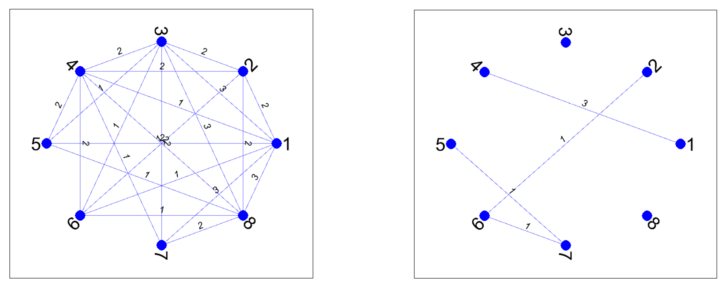
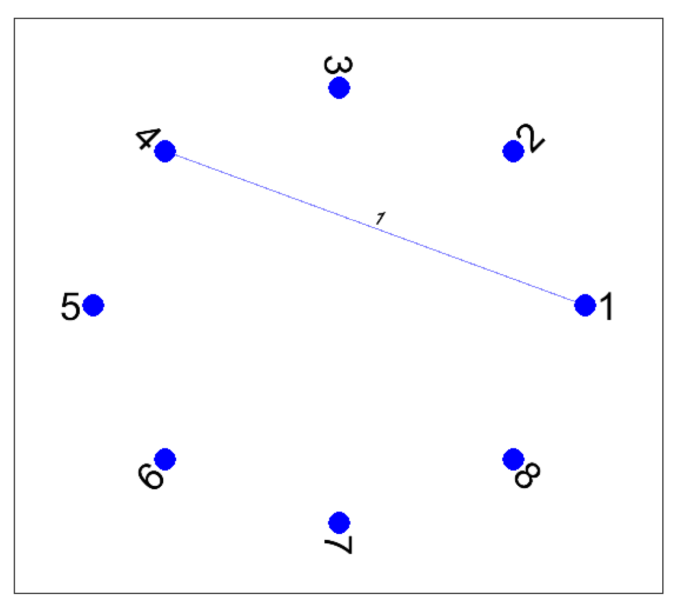
Another contribution of Theorem 1 and Definition 6 is that they are useful to describe the behavior of the series of m rankings in terms of a competitivity graph. We can define a weighted graph for each one of the interactions between the elements when passing from ${\mathbf{a}}_i$ to ${\mathbf{a}}_{i+1}$: crossings, passing from tie to untie (or vice-versa), and crossing after ties. Moreover, for each kind of graph, we can add the contributions of all the pairs of consecutive rankings to obtain a projected graph for any interaction (crossings, passing from tie to untie (or vice-versa), and crossing after ties). The procedure is the following: First, we construct an undirected graph for each pair of rankings ${\mathbf{a}}_k,{\mathbf{a}}_{k+1}$ by identifying each element i as a node and defining an edge between i and j by the rule: there is an edge connecting $\{i,j\}$ with weight ${\overline{K}}_{i,j}^{(p,q)}({\mathbf{a}}_k,{\mathbf{a}}_{k+1})$ when this weight is nonzero. By adding the $m-1$ pairs of undirected graphs we obtain a projected graph with a total sum of weights $K_{cev}^{(p=0.5,q=0)}({\mathbf{a}}_1,\dots ,{\mathbf{a}}_m)$. By adding the crossing after ties term to the projected graph we have all the ingredients appearing on Definition 6. We show this procedure by using the next example with $m=6$ and $n=8$.

Example 10.

Given the series of incomplete rankings with ties

$$\begin{array}{cccccc}{\mathbf{r}}_1& {\mathbf{r}}_2& {\mathbf{r}}_3& {\mathbf{r}}_4& {\mathbf{r}}_5& {\mathbf{r}}_6\\ 5& 2& 4& 6& 2& 1\\ 7& 1& 8& 1,4& 1,4& 5\\ 3& 8& 3& 3& 6,7& 8\\ 8& 3& 2,6& 8& 5& 3\\ 1,4& 5,7& 5,7& 2& 3& 4\\ & 4& 1& 7& 8& \end{array}$$

the corresponding ${\mathbf{a}}_i$ are

$$\begin{array}{cccccc}{\mathbf{a}}_1& {\mathbf{a}}_2& {\mathbf{a}}_3& {\mathbf{a}}_4& {\mathbf{a}}_5& {\mathbf{a}}_6\\ 5& 2& 6& 2& 2& 1\\ •& 1& 4& 5& 1& •\\ 3& 4& 3& 3& 5& 4\\ 5& 6& 1& 2& 2& 5\\ 1& 5& 5& •& 4& 2\\ •& •& 4& 1& 3& •\\ 2& 5& 5& 6& 3& •\\ 4& 3& 2& 4& 6& 3\end{array}$$

In this example we have $n=8$, and an easy computation leads to the parameters shown in

Table 4. Parameters for pairs of consecutive rankings. Example 10.

	${\mathbf{a}}_1\to {\mathbf{a}}_2$	${\mathbf{a}}_2\to {\mathbf{a}}_3$	${\mathbf{a}}_3\to {\mathbf{a}}_4$	${\mathbf{a}}_4\to {\mathbf{a}}_5$	${\mathbf{a}}_5\to {\mathbf{a}}_6$
$n_{••}$	1	0	0	0	0
$n_{•\ast }$	1	1	0	1	0
$n_{\ast •}$	0	0	1	0	3
$n_{\ast \ast }$	6	7	7	7	5
s	9	12	8	9	4
$n_{tu}$	2	0	2	1	1
$n_{tt}$	0	0	0	0	0
$N_{inc}$	13	7	7	7	18
$\overline{n}$	6	7	7	7	5
${\widehat{\tau }}_{ev}^{•}$	−0.3333	−0.1429	0.1429	0.0952	0.1000
${\widehat{NS}}^{•}$	0.6667	0.5714	0.4268	0.4524	0.4500
${\tau }_{ev}^{•}$	−0.1786	−0.1071	0.1071	0.0714	0.0357
$N{S}^{•}$	0.5893	0.5536	0.4464	0.4643	0.4821
${\tau }_x$	−0.1786	−0.1071	0.1071	0.0714	0.0357
${\widehat{\tau }}_x$	−0.3333	−0.1429	0.1429	0.0952	0.1000

. For each pair of consecutive rankings it is easy to compute the parameters defined in Theorem 1: $n_{••}$, $n_{•\ast }$, $n_{\ast •}$, $n_{\ast \ast }$, s, $n_{tu}$, and $n_{tt}$. Then, by using Equation (10) in Theorem 1 we can obtain, for any pair of rankings, the value $N_{inc}$. $\overline{n}$ is the number of common elements, given by (9). The coefficient ${\tau }_{ev}^{•}$ is given by (35) , and the coefficient ${\widehat{\tau }}_{ev}^{•}$ is given by (36). In analogy with (4) we can define the corresponding normalized mean strengths given by

$$N{S}^{•}=\frac{(1-{\tau }_{ev}^{•})}{2}$$

(38)

and

$${\widehat{NS}}^{•}=\frac{(1-{\widehat{\tau }}_{ev}^{•})}{2}$$

(39)

Finally, in Table 4 we include the coefficients ${\tau }_x$ and ${\widehat{\tau }}_x$ given by (7) and (8), respectively. These last coefficients are included to show that our new coefficients ${\tau }_{ev}^{•}$ and ${\widehat{\tau }}_{ev}^{•}$ reduce to them when only a pair of rankings are considered.

To compute our new coefficients ${\tau }_{ev}^{•}$ and ${\widehat{\tau }}_{ev}^{•}$ for the whole series of rankings ${\mathbf{a}}_1$ to ${\mathbf{a}}_6$ we need some previous parameters. First, we need the value

$$\sum _{i=1}^5{N}_{inc}({\mathbf{a}}_i,{\mathbf{a}}_{i+1})=52$$

To compute $K_{cev}^{(p=0.5,q=0)}({\mathbf{a}}_1,\dots ,{\mathbf{a}}_6)$, given by (31), we need to know, previously, the value of the crossing after ties coefficients ${\overline{K}}_{i,j}^{cat}({\mathbf{a}}_1,\dots ,{\mathbf{a}}_6)$, given by Definition 3. Note that the unique long crossing occurs for the pair $\{1,4\}$: the elements tagged as 1 and 4 are such that 4 is above 1 in ${\mathbf{r}}_{\mathbf{3}}$, both elements are tied in rankings ${\mathbf{r}}_4$ and ${\mathbf{r}}_5$, and, finally, 4 is below 1 in ranking ${\mathbf{r}}_6$. Note, for example, that the pair $\{5,7\}$ does not accomplish the conditions of crossing after ties. Therefore the only term that contributes to ${\sum }_{\{i,j\}}{\overline{K}}_{i,j}^{cat}$ is ${\overline{K}}_{1,4}^{cat}({\mathbf{a}}_1,\dots ,{\mathbf{a}}_6)=1$.

With respect to $K_{ev}^{(p=0.5,q=0)}({\mathbf{a}}_1,\dots ,{\mathbf{a}}_6)$, given by (30), we need to compute the terms ${\overline{K}}_{i,j}^{(p,q)}({\mathbf{a}}_{\mathbf{i}},{\mathbf{a}}_{\mathbf{i}+\mathbf{1}})$, given by (28), for any pair of consecutive rankings. A detailed computation shows that, in this example, we have 42 crossings and 6 cases of tie to untie or viceversa. The precise pairs of elements that contribute to these cases are shown in the corresponding projected weighted graphs in Figure 1. The crossing after ties case is represented in Figure 2.

Therefore we have all the ingredients to compute $K_{cev}^{(p=0.5,q=0)}$. That is

$$\begin{array}{ccc}\hfill K_{cev}^{(p=0.5,q=0)}({\mathbf{a}}_1,\dots ,{\mathbf{a}}_6)& =& K_{ev}^{(p=0.5,q=0)}({\mathbf{a}}_1,\dots ,{\mathbf{a}}_6)+\sum _{\{i,j\}}{\overline{K}}_{i,j}^{cat}({\mathbf{a}}_1,\dots ,{\mathbf{a}}_6)\hfill \\ & =& \sum _{i=1}^5{K}^{(p,q)}({\mathbf{a}}_i,{\mathbf{a}}_{i+1})+\sum _{\{i,j\}}{\overline{K}}_{i,j}^{cat}({\mathbf{a}}_1,\dots ,{\mathbf{a}}_6)\hfill \\ \hfill \end{array}$$

and, by Remark (7), we know that

$$K_{i,j}^{(p,q)}(\mathbf{a},\mathbf{b})=s+p{n}_{tu}+q{n}_{tt}$$

Therefore, we have

$$\begin{array}{ccc}\hfill K_{cev}^{(p=0.5,q=0)}({\mathbf{a}}_1,\dots ,{\mathbf{a}}_6)& =& (9+12+8+9+4)+0.5(2+0+2+1+1)+{\overline{K}}_{1,4}^{cat}({\mathbf{a}}_1,\dots ,{\mathbf{a}}_6)\hfill \\ & =& 42+3+1=46.\hfill \\ \hfill \end{array}$$

By using (35), we obtain

$${\tau }_{ev}^{•}=1-\frac{4·46+2·52}{(6-1)8·7}=1-1.0286=-0.0286$$

that corresponds to an equivalent normalized mean strength

$$N{S}^{•}=\frac{(1-{\tau }_{ev}^{•})}{2}=0.5143$$

Finally, regarding ${\widehat{\tau }}_{ev}^{•}$, we have

$${\widehat{\tau }}_{ev}^{•}=1-\frac{2·46}{\frac{1}{2}(6·5+7·6+7·6+7·6+5·4)}=1-\frac{4·46}{176}=-0.0455$$

that corresponds to

$${\widehat{NS}}^{•}=0.5227.$$

All in all, we conclude that ${\widehat{\tau }}_{ev}^{•}$ is a proper coefficient for the evaluation of m incomplete rankings with ties and can be considered as a natural extension of the coefficient ${\widehat{\tau }}_x$ presented in [12]. In the next section we apply the new coefficients ${\tau }_{ev}^{•}$ and ${\widehat{\tau }}_{ev}^{•}$ to real rankings appearing on Spotify charts.

7. Results

Spotify is one of the major music streaming services worldwide, with 299 million monthly active users, as of July 2020 [28]. The company Spotify Technology S.A. has been listed on the New York Stock Exchange since 2018. As of September 2020, the company offers a catalog of 60 million tracks and operates in 92 countries from Albania to Vietnam [29]. Spotify divides the monthly active users into four regions [30]: Europe (35%), North America (26%), Latin America (22%) and rest of the world (17%). The app is available on several devices, such as computers, smartphones, tablets, wearable devices, etc. The users can choose between a free service (called Freemium or Ad-Supported) or a Premium service. In any case, the user can listen by streaming any song of the catalog (that is, the user does not own the song’s digital file, but can listen to it). It is accepted that music streaming services have transformed the entire music market—see [31]—and they have evolved very fast, changing their services and capabilities. For example, Spotify has signed some partnerships with Microsoft [32], Sony [33] and Facebook [34] among other big companies. There exists a large amount of literature about Spotify, but it is mainly focused on Economics and Music. To the best of our knowledge, a small number of papers are devoted to the mathematical aspects of the rankings produced by Spotify. Among these papers, we have [35,36]. A paper that studies the relationship between personality and type of music is [37]. See [38] for more details about Spotify.

Like other services on the Internet, Spotify provides some chart lists (song rankings) based on the platform’s number of streamings. To this kind of rankings belongs the Top 200 (see [39,40,41]), that is one of the topics of our study. Another ranking that we are interested in is called Viral 50 which is an evolution of the original Social 50 ranking (see [42,43,44]) that incorporated in the song chart the effect of the social sharing of a track by Spotify users. This sharing included platforms such as Facebook and Twitter. It is not completely clear for us how this rank is computed, but it aims to gather fresh songs that acquire high impact on social networks by new release promotions, special apparitions on tv-shows, music festivals, tours, etc. (see [45] for an example of how a viral song transformed into a Top 100 song in 2013).

Due to the situation caused by the COVID-19 pandemic, the live music business reflected some drawbacks, such as festivals being cancelled worldwide, a reduction in public-performance licensing, and other related factors—see [46]. As an example, Warner Music Group Corp showed a total revenue fall of $1.7\%$ in the first quarter of 2020 compared to the first quarter of 2019 [47]. Spotify also reported some impact on their business, but in the first quarter of 2020, it seemed that the consumption recovered and monthly active users increased faster in the first quarter of 2020 than in the same period of 2019 [30]. Some perturbations in Spotify streaming were also reported by the music analytic company Chartmetric that observed a change in the type of consumption of Spotify streamings by music genre in the period between 3 March 2020 to 9 April 2020, concluding that it seemed that it had been a pandemic-induced lifestyle change [48].

With regard to the Top 50 viral, it is reasonable to think that the fact that many artists (such as Lady Gaga, Alicia Keys, and Cardi B. [46]) have postponed big releases may have decreased the movements in these charts.

7.1. Method to Convert Spotify Lists into Incomplete Rankings

Both Spotify Top 200 and Viral 50 lists can be treated as incomplete rankings since some elements (songs) quit the list and some others that appear on the list (new songs). Let us call any of these rankings as Top k rankings. In order to handle these Top k rankings, our methodology consists of the following steps:

1.

Select a set of m lists $\{{\mathbf{v}}_1,{\mathbf{v}}_2,\dots ,{\mathbf{v}}_m\}$ with k entries in each ${\mathbf{v}}_i$.

2.

Denote as n the number of different songs that appear on these m lists. We tag these songs from 1 to n, following the order they first appear, reading the lists from the first to the last one, and each list from top to bottom. Denote ${\mathbf{t}}_i$ the tagged version of ${\mathbf{v}}_i$, for $i=1,2,\dots ,m$, including all the n songs.

3.

Denote ${\mathbf{r}}_1$ a vector with entries from 1 to n. The first k values correspond to the elements in ${\mathbf{v}}_1$.

4.

Construct the rankings ${\mathbf{r}}_i$ for $2=1,\dots m$, in the following form:

(a)

The first k entries of ${\mathbf{r}}_i$ are copied from ${\mathbf{t}}_i$;

(b)

The rest of the entries form a vector ${\mathbf{s}}_i$ and come from the the elements that quit from ${\mathbf{t}}_{i-1}$ plus the elements that, being in ${\mathbf{s}}_{i-1}$, are not included in ${\mathbf{t}}_i$.

These $n-k$ elements preserve their relative order. This order is not important since these elements are not included in the Top k ranking ${\mathbf{t}}_i$.

5.

From each ${\mathbf{t}}_i$, we construct the corresponding incomplete ranking ${\mathbf{a}}_i$ given by (5).

Example 11.

Let us consider three Top 4 lists (${\mathbf{v}}_1,{\mathbf{v}}_2,{\mathbf{v}}_3$) and construct the corresponding three rankings (${\mathbf{a}}_1,{\mathbf{a}}_2,{\mathbf{a}}_3$). Here we have $m=3$ and $k=4$.

$$\left|\begin{array}{c}\begin{array}{ccc}{\mathbf{v}}_1& {\mathbf{v}}_2& {\mathbf{v}}_3\end{array}\\ \begin{array}{ccc}A& B& F\\ B& C& C\\ C& E& B\\ D& A& E\end{array}\end{array}\right|\to \begin{array}{c}\begin{array}{ccc}& & \\ {\mathbf{t}}_1& {\mathbf{t}}_2& {\mathbf{t}}_3\\ & & \end{array}\\ \begin{array}{ccc}& & \\ {\mathbf{s}}_1& {\mathbf{s}}_2& {\mathbf{s}}_3\end{array}\end{array}\begin{array}{c}\begin{array}{ccc}{\mathbf{r}}_1& {\mathbf{r}}_2& {\mathbf{r}}_3\end{array}\\ \left\{\begin{array}{c}\begin{array}{c}\begin{array}{ccc}1& 2& 6\\ 2& 3& 3\\ 3& 5& 2\\ 4& 1& 5\end{array}\end{array}\end{array}\right\}\\ \left\{\begin{array}{c}\overline{\begin{array}{ccc}5& 4& 1\end{array}}\\ \begin{array}{ccc}6& 6& 4\end{array}\end{array}\right\}\end{array}⟶\begin{array}{ccc}{\mathbf{a}}_1& {\mathbf{a}}_2& {\mathbf{a}}_3\\ 1& 4& •\\ 2& 1& 3\\ 3& 2& 2\\ 4& •& •\\ •& 3& 4\\ •& •& 1\end{array}$$

We have denoted as ${\mathbf{s}}_i$ the elements beyond the k position in each ranking ${\mathbf{r}}_i$. The rankings ${\mathbf{a}}_i$ are constructed looking at ${\mathbf{r}}_i$ from positions 1 to 4. Since the elements that do no belong to ${\mathbf{t}}_i$ are in ${\mathbf{s}}_i$, we tagged them as •.

7.2. Comparison of Two Series of Top 200 Rankings

From the site [49] we downloaded the series of Top 200 (Global) rankings corresponding to the following time intervals:

• 2019 Series: 18 weekly rankings ranging from 28 December 2018 to 3 May 2019.
• 2020 Series: 18 weekly rankings ranging from 27 December 2019 to 1 May 2020.

The term Global means that the charts were produced from streaming on Spotify from all over the world. By using the methodology explained in the previous section, we convert the 18 downloaded rankings to a series of incomplete rankings (with no ties) ${\mathbf{a}}_1,\dots ,{\mathbf{a}}_{18}$, and we compute our parameters. This is repeated for each considered year. The results are shown in

Table 5. Parameters for two series of incomplete rankings obtained from Spotify Top 200 lists.

	2019 Series	2020 Series
n	474	556
$N_{inc}$	$1.6\times {10}^6$	$2.4\times {10}^6$
$<{\overline{n}}_{i,i+1}>$	182	175
${\tau }_{ev}^{•}$	0.1256	0.0836
$N{S}^{•}$	0.4372	0.4582
${\widehat{\tau }}_{ev}^{•}$	0.8540	0.8421
${\widehat{NS}}^{•}$	0.0730	0.0789

.

In Table 5 we have denoted by $<{\overline{n}}_{i,i+1}>$ the average of $\left\{{\overline{n}}_{i,i+1}\right\}$ for $i=1,2,\dots ,17$, that is the mean number of common elements from each pair of consecutive rankings. We see that the number of songs involved in the 2019 series is $n=474$, which is lower than the 2020 series number. This fact could indicate that there was more activity in the 2020 series since more new songs appeared than the previous year. By extension, we can also conclude that the activity on Spotify of the users was higher in the 2020 series.

The same tendency is observed by looking at $N_{inc}$ and ${\overline{n}}_{i,i+1}$. Our coefficients $N{S}^{•}$ and ${\widehat{NS}}^{•}$ corroborate this intuition since they take higher values in the 2020 Series than in the 2019 Series. Analogously, by looking at ${\tau }_{ev}^{•}$ and ${\widehat{\tau }}_{ev}^{•}$, we see a decrease when comparing the 2019 Series with the 2020 Series. Recall that the coefficients $N{S}^{•}$ and ${\widehat{NS}}^{•}$ introduced in this paper offer a measure of the movements in the rankings, since they take into account the number of crossings and, in this case, that we do not have ties, due to the effect of absent elements.

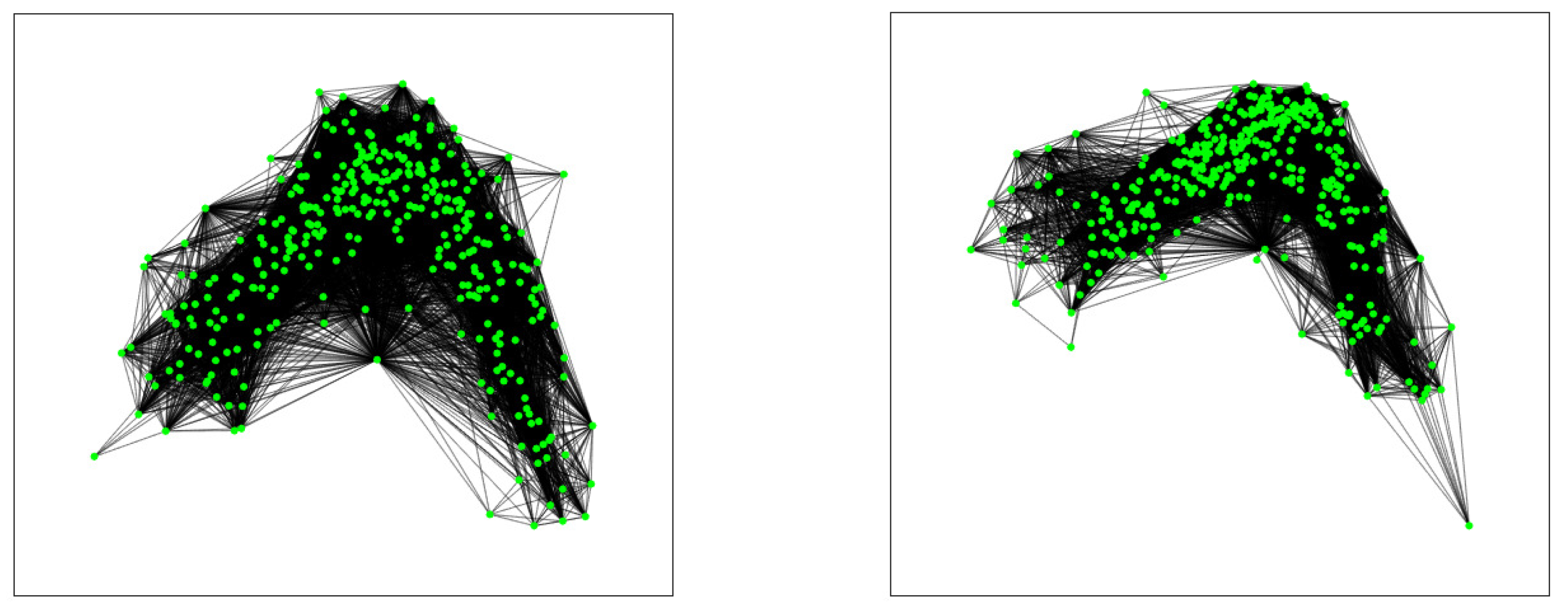
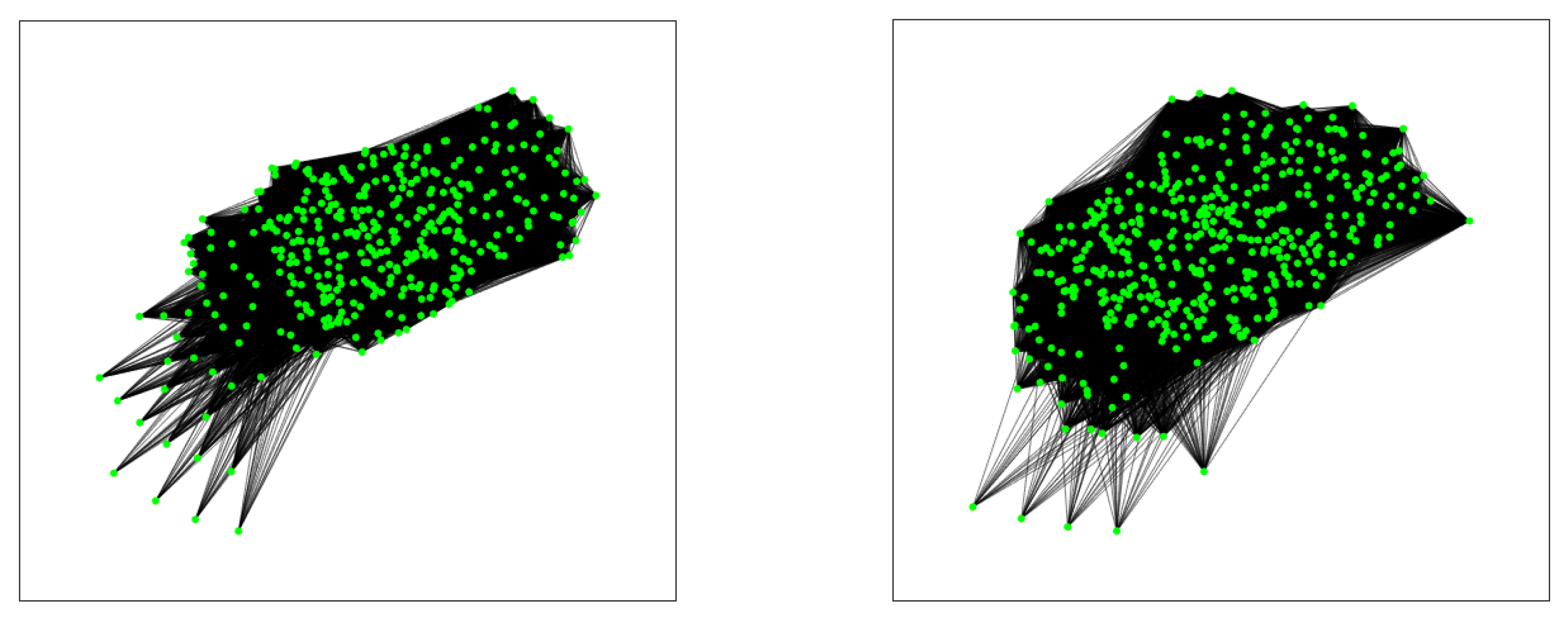
In the same manner, as we did in Example 10, we can construct the projected graph corresponding to the crossings for each series. We show these graphs in Figure 3, that have been plotted with MATLAB by using the option ”subspace”.

7.3. Comparison of Two Series of Viral-50 Rankings

From the site [50], we downloaded the series of Viral 50 (Global) weekly rankings corresponding to the following periods:

• 2019 Series: 18 weekly rankings ranging from 3 January 2019 to 2 May 2019.
• 2020 Series: 18 weekly rankings ranging from 2 January 2020 to 30 April 2020.

For each considered year, we convert the 18 downloaded rankings to a series of incomplete rankings (with no ties) ${\mathbf{a}}_1,\dots ,{\mathbf{a}}_{18}$, and we computed again the aforementioned parameters. The results are shown in

Table 6. Parameters for two series of incomplete rankings obtained from Spotify Viral 50 lists.

	2019 Series	2020 Series
n	315	300
$N_{inc}$	$8.3\times {10}^5$	$7.5\times {10}^5$
$<{\overline{n}}_{i,i+1}>$	33.6	35
${\tau }_{ev}^{•}$	0.0067	0.0093
$N{S}^{•}$	0.4966	0.4954
${\widehat{\tau }}_{ev}^{•}$	0.6037	0.6922
${\widehat{NS}}^{•}$	0.1982	0.1539

.

The number of songs involved in the 2019 series is $n=315$, that is greater than the number involved in the 2020 series. This fact could indicate that there was less viral activity in the 2020 series since fewer new songs appeared than the previous year. The same tendency is observed at $N_{inc}$. This intuition is corroborated by our coefficients. $N{S}^{•}$ and ${\widehat{NS}}^{•}$ since they take lower values in the 2020 series than in the 2019 series. We also see an increase in ${\tau }_{ev}^{•}$ and ${\widehat{\tau }}_{ev}^{•}$ when comparing the 2019 series with the 2020 series.

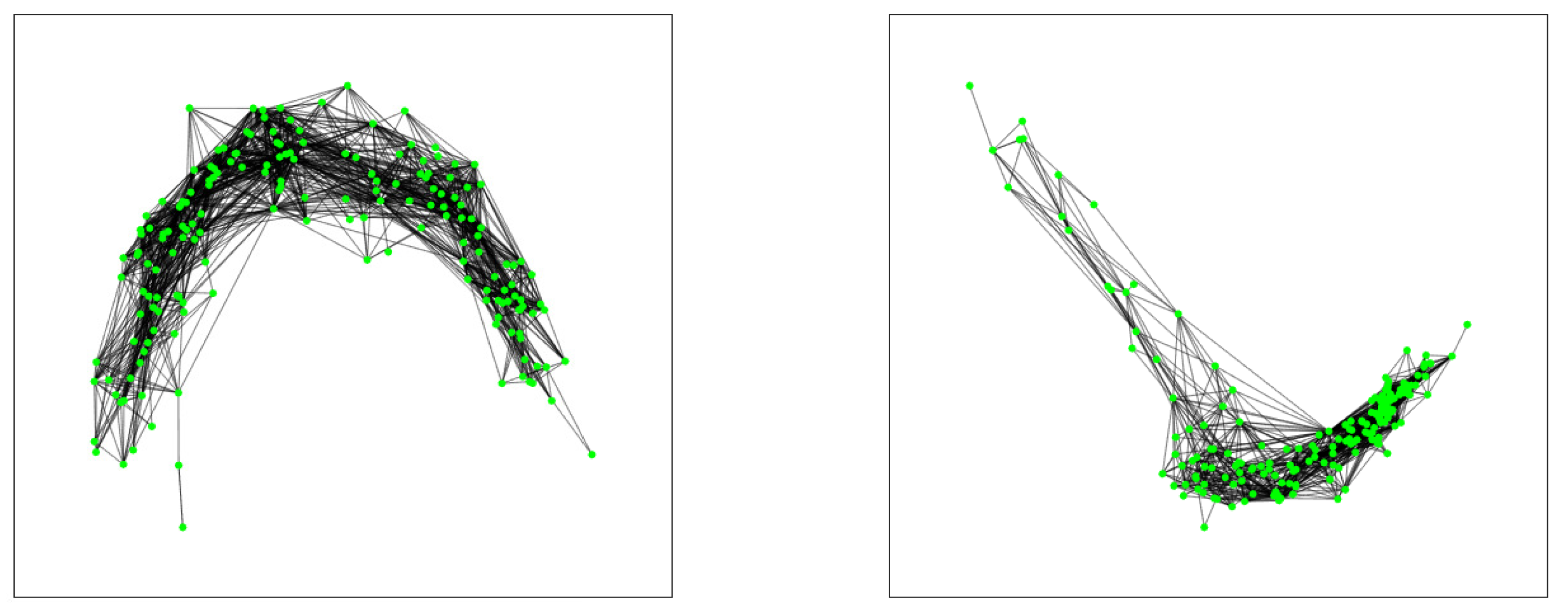
If we compare these results with those obtained in the previous section, we conclude that Spotify’s viral activity was negatively affected by the Pandemic. This may seem reasonable since many events that produce sharing in Social Networks, such as shows, new releases, and performances, were postponed during these months, as we have already discussed. We again plot the projected graph corresponding to the crossings for each series in Figure 4.

7.4. Comparison of a Series of Top 200 and a Series of Viral 50 Rankings

Given that our coefficients ${\tau }_{ev}^{•}$, ${\widehat{\tau }}_{ev}^{•}$, $N{S}^{•}$, and ${\widehat{NS}}^{•}$ are normalized, we can compare series of rankings of different type. Looking at Table 5 and Table 6, we conclude (e.g., looking at ${\widehat{NS}}^{•}$) that the Viral-50 rankings present more activity than the Top 200 rankings. For example in the 2019 series the value of ${\widehat{NS}}^{•}$ is $0.1982$ for the Viral-50 rankings, and only $0.0730$ for the Top 200 rankings. This conclusion seems reasonable, taking into account that the Viral-50 rankings are constructed by looking at the behaviours of songs that may rapidly change, since they are viral phenomena.

7.5. Comparison of the Evolution of Two Series of Incomplete Ranking with Ties

Spotify charts Top 200 do not present ties, but we can construct incomplete rankings with ties if we take into account the Top 200 ranking and the rest of the songs that appear in the whole studied interval. In detail, to obtain a series of incomplete rankings with ties from a Top 200 series on Spotify, we will consider the whole list of tracks along with the m rankings and focus on what happens in positions greater than 200. Using the terminology used in Example 11 we consider the elements that appear on the rankings, denoted as ${\mathbf{s}}_1$, ${\mathbf{s}}_2,\dots$. In this ranking we consider the following:

(i)

All the tracks in ${\mathbf{s}}_1$ are tied. That is ${\mathbf{a}}_1=\left[{•}_{1,200}{\mathbf{1}}^{n-200}\right]$ where ${•}_{1,200}$ is a row vector of 200 entries of the type •, and ${\mathbf{1}}^{n-200}$ is the row vector of all-ones, with $n-200$ entries, being n the total number of different tracks in the m rankings.

(ii)

For $i=2,3\dots m$, we consider that in ${\mathbf{s}}_i$ we have (at most) two buckets of tied elements. In one bucket we have the elements (if any) that come from ${\mathbf{t}}_{i-1}$. In the other bucket, we consider the rest of the elements of ${\mathbf{s}}_i$

The next example with a series of $m=7$ Top 4 charts illustrates this methodology.

Example 12.

Let us consider the series of seven Top 4 tracks ${\mathbf{v}}_i$ with $n=10$ elements $\{A,B,\dots ,J\}$ given by the rankings

$$\begin{array}{ccccccc}A& A& F& G& G& G& J\\ B& B& E& H& H& I& C\\ C& E& A& C& C& B& A\\ D& F& C& E& E& A& H\end{array}$$

from these rankings we construct the rankings ${\mathbf{t}}_i$ and ${\mathbf{s}}_i$ to obtain the rankings in the form

$$\begin{array}{cc}\begin{array}{c}\begin{array}{c}\end{array}{\mathbf{t}}_i\\ \\ \\ \\ {\mathbf{s}}_i\\ \\ \\ \end{array}& \begin{array}{ccccccc}1& 1& 6& 7& 7& 7& 10\\ 2& 2& 5& 8& 8& 9& 3\\ 3& 5& 1& 3& 3& 2& 1\\ 4& 6& 3& 5& 5& 1& 8\\ 5& 3& 2& 6& 6& 8& 7\\ 6& 4& 4& 1& 1& 3& 9\\ 7& 7& 7& 2& 2& 5& 2\\ 8& 8& 8& 4& 4& 6& 5\\ 9& 9& 9& 9& 9& 4& 6\\ 10& 10& 10& 10& 10& 10& 4\end{array}\end{array}$$

Now, we consider the rankings ${\mathbf{s}}_i$ as a series of incomplete rankings with ties with the convention explained above and we compute the corresponding ${\mathbf{a}}_i$ vectors to obtain the rankings

$$\begin{array}{ccccccc}{\mathbf{a}}_1& {\mathbf{a}}_2& {\mathbf{a}}_3& {\mathbf{a}}_4& {\mathbf{a}}_5& {\mathbf{a}}_6& {\mathbf{a}}_7\\ •& •& •& 1& 1& •& •\\ •& •& 1& 2& 1& •& 1\\ •& 1& •& •& •& 1& •\\ •& 1& 2& 2& 1& 2& 2\\ 1& •& •& •& •& 1& 2\\ 1& •& •& 1& 1& 2& 2\\ 1& 2& 2& •& •& •& 1\\ 1& 2& 2& •& •& 1& •\\ 1& 2& 2& 2& 1& •& 1\\ 1& 2& 2& 2& 1& 2& •\end{array}$$

Note that, since there are at most two buckets, the entries of ${\mathbf{a}}_i$ belong to the set $\{1,2,•\}$. Note also that in ${\mathbf{s}}_5$ there is only one bucket.

By using this methodology, we have converted the series of rankings studied in Section 7.2 to the corresponding series ${\mathbf{a}}_i$ with ties. The parameters obtained are shown in

Table 7. Series of incomplete rankings with ties obtained from Spotify Top 200 charts.

	2019 Series	2020 Series
n	474	556
$N_{inc}$	$1.4\times {10}^6$	$1.7\times {10}^6$
$<{\overline{n}}_{i,i+1}>$	256	331
${\tau }_{ev}^{•}$	0.2577	0.3108
$N{S}^{•}$	0.3712	0.3446
${\widehat{\tau }}_{ev}^{•}$	0.8848	0.8757
${\widehat{NS}}^{•}$	0.0576	0.0621

.

If we look at n, $N_{inc}$, $<{\overline{n}}_{i,i+1}>$, and ${\widehat{NS}}^{•}$ in Table 7, we conclude that there has been more activity in the 2020 Series than in the 2019 Series. However, by looking at ${NS}^{•}$ (and ${\tau }_{ev}^{•}$), the conclusion seems to be the reverse. Here we see, therefore, that ${\tau }_{ev}^{•}$ and ${\widehat{\tau }}_{ev}^{•}$ can present different tendencies. This is related to the form in which they are normalized, as we have commented in Remark 5 and in Section 6. These results provide an example of how the transformation from ${\tau }_{ev}^{•}$ to ${\widehat{\tau }}_{ev}^{•}$ is not linear, since ${\tau }_{ev}^{•}$ increases from 2019 to 2020 but ${\widehat{\tau }}_{ev}^{•}$ decreases in the same period.

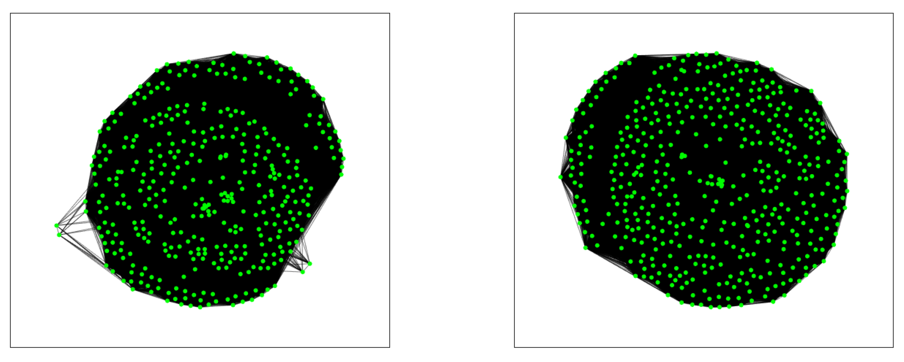
In Figure 5, we show the plot of the giant component corresponding to the projected graph showing the interactions of the form tie to untie or viceversa. That is, there is a link between elements (nodes) i and j when the pair $\{i,j\}$ goes from tie to untie (or vice versa) in any pair of consecutive rankings ${\mathbf{a}}_i$ and ${\mathbf{a}}_{i+1}$. We see many more interactions of this type in the 2020 series than in the 2019 series.

In Figure 6, we show the plot of the giant component corresponding to the projected graph showing the interactions of the form tie to tie, that is, there is a link between elements (nodes) i and j when the pair $\{i,j\}$ goes from tie to tie in any pair of consecutive rankings ${\mathbf{a}}_i$ and ${\mathbf{a}}_{i+1}$. We also see many more interactions of this type in the 2020 series than in the 2019 series.

Therefore, and taking into account the values of Table 7, we can conclude (for this artificial model of incomplete ranking with ties) that there was more activity in the 2020 series than in the 2019 series.

We have shown the application of the new coefficients introduced in this work, as long as the utility of the visualizations based on the projected graph plots of the (evolutive) competitive graph associated to a series of incomplete rankings with or without ties.

8. Conclusions

We present the main conclusions of our work:

• We provide a theoretical result that allows for understanding, in terms of the type of interactions between pairs of elements in a series of incomplete rankings with ties, two recently introduced coefficients, given in [4,12].
• We have defined two new coefficients to characterize a series of incomplete rankings with ties in terms of the interactions mentioned above.
• We have presented a methodology to treat Spotify charts (both Top 200 and Viral 50) as a series of incomplete rankings. This methodology allows us to obtain conclusions about the movements in the lists and, therefore, on the activity of the users of the app.
• We have obtained an artificial series of incomplete rankings with ties based on Spotify Top 200 lists, to apply our coefficients and show the applicability of the method.
• The main theoretical result (Theorem 1) may serve to define new coefficients by giving weight to the interactions between pairs of elements when going from one ranking to the next one. The applications can be of interest in other fields (neuroscience, sports, bioinformatics, etc.).