Transboundary Basins Need More Attention: Anthropogenic Impacts on Land Cover Changes in Aras River Basin, Monitoring and Prediction


 , ,
, ,  ,
,
Abstract
:1. Introduction
2. Materials and Methods
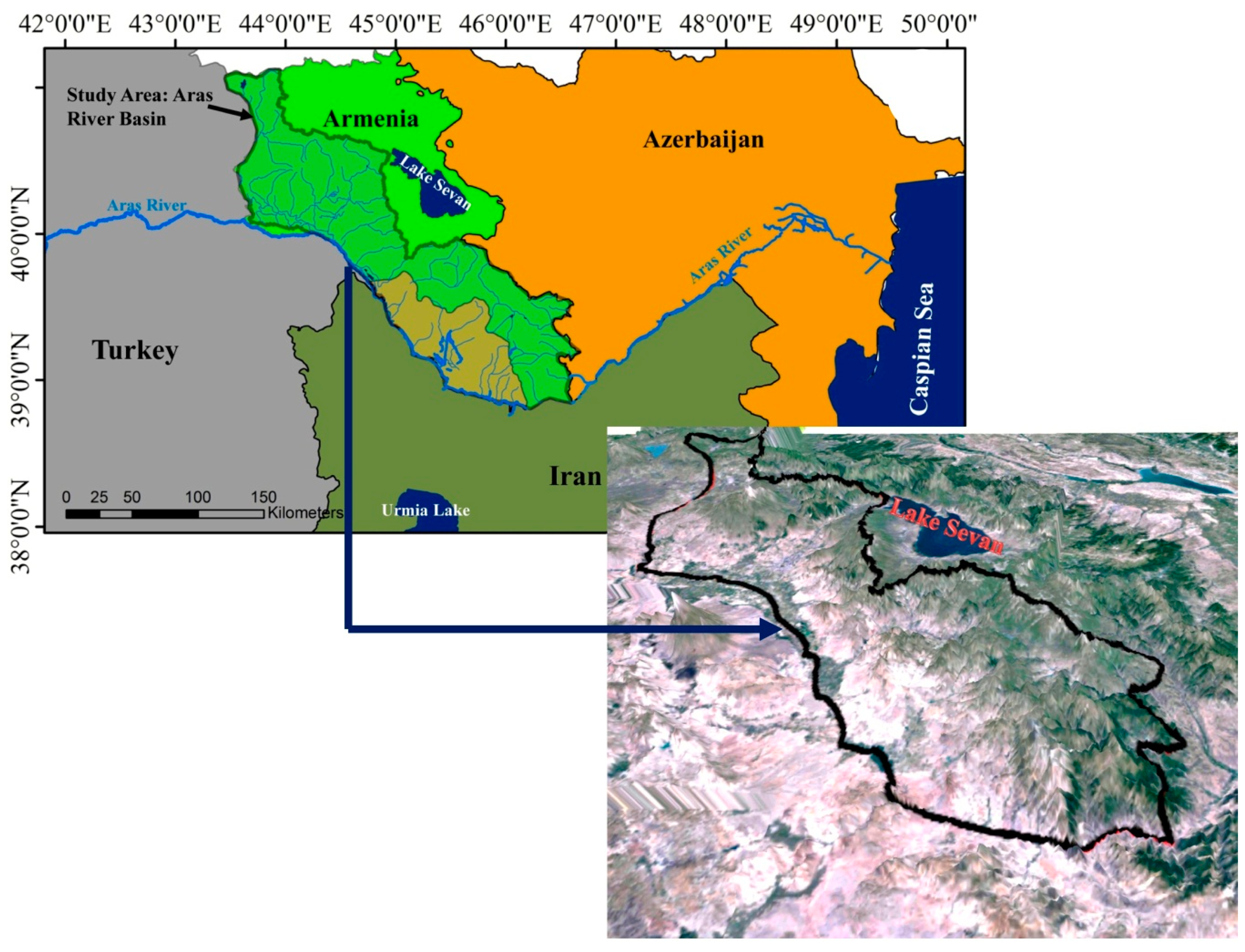
2.1. Study Area
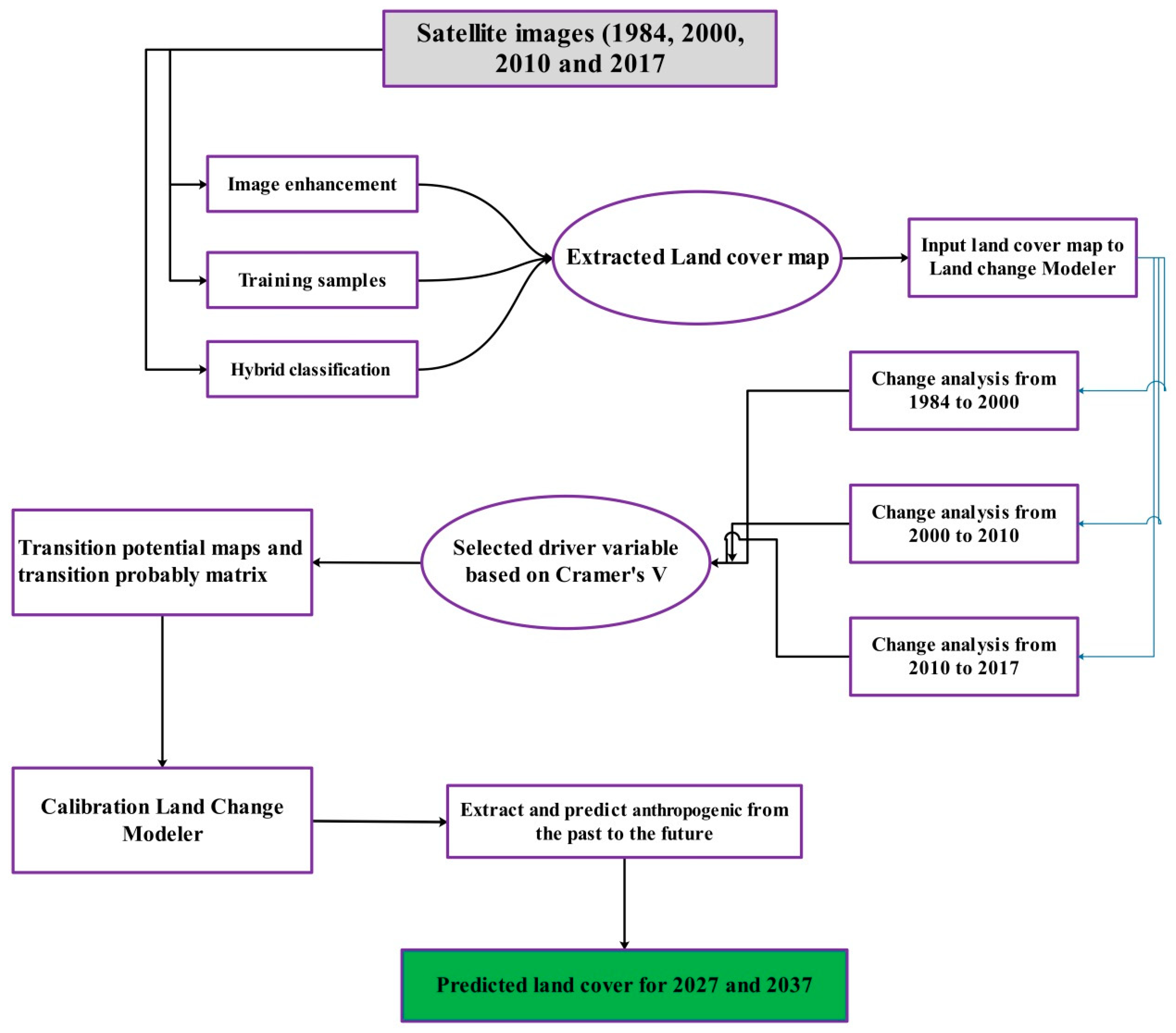
2.2. Overview of Data Collection and Research Methods
2.2.1. Preparing Satellite Image and Preprocessing
2.2.2. Producing LC Maps and Accuracy Assessment
2.2.3. Land Cover Change Prediction
2.2.4. Details of Sub-Models
3. Results
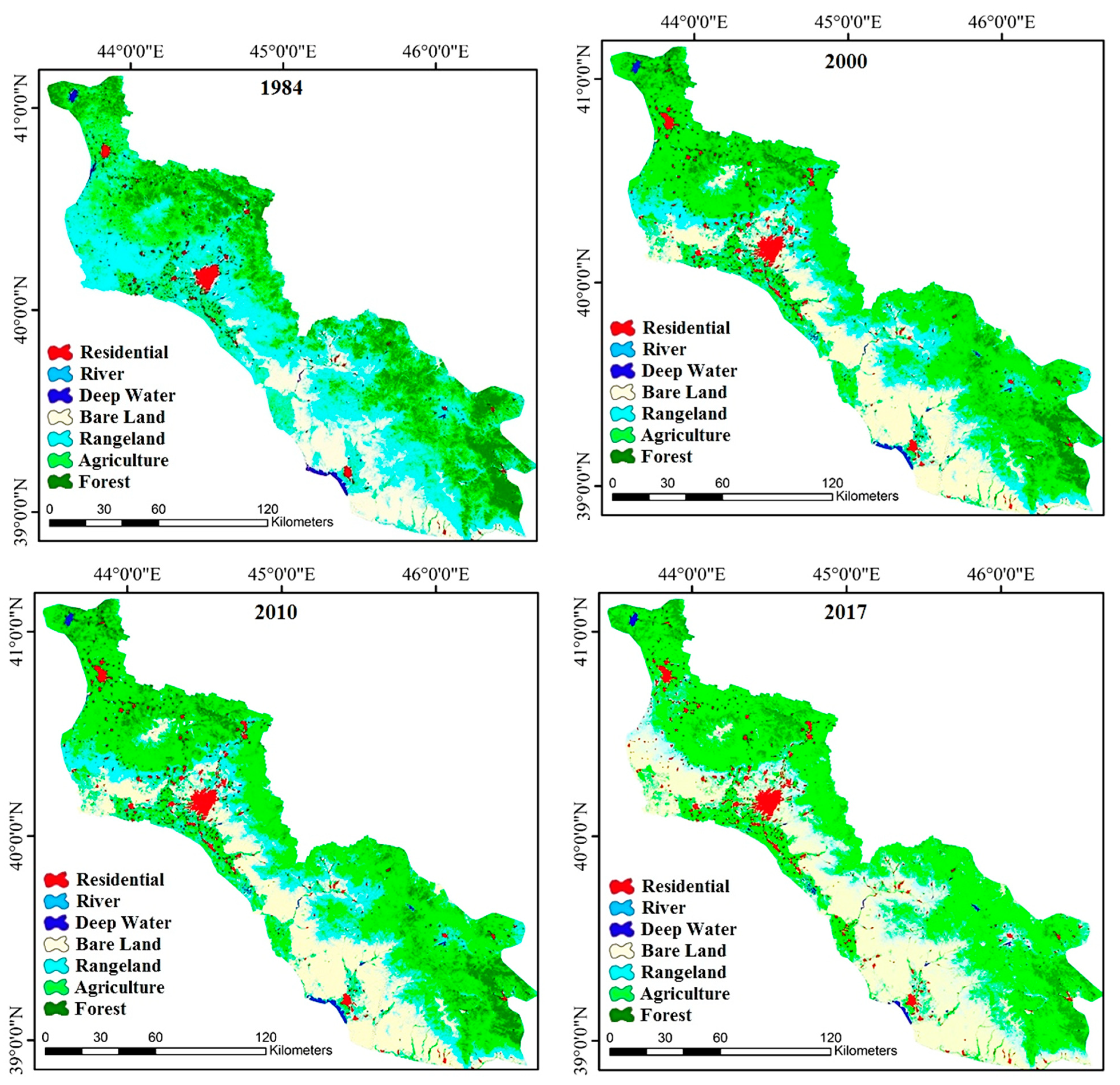
3.1. LC Maps
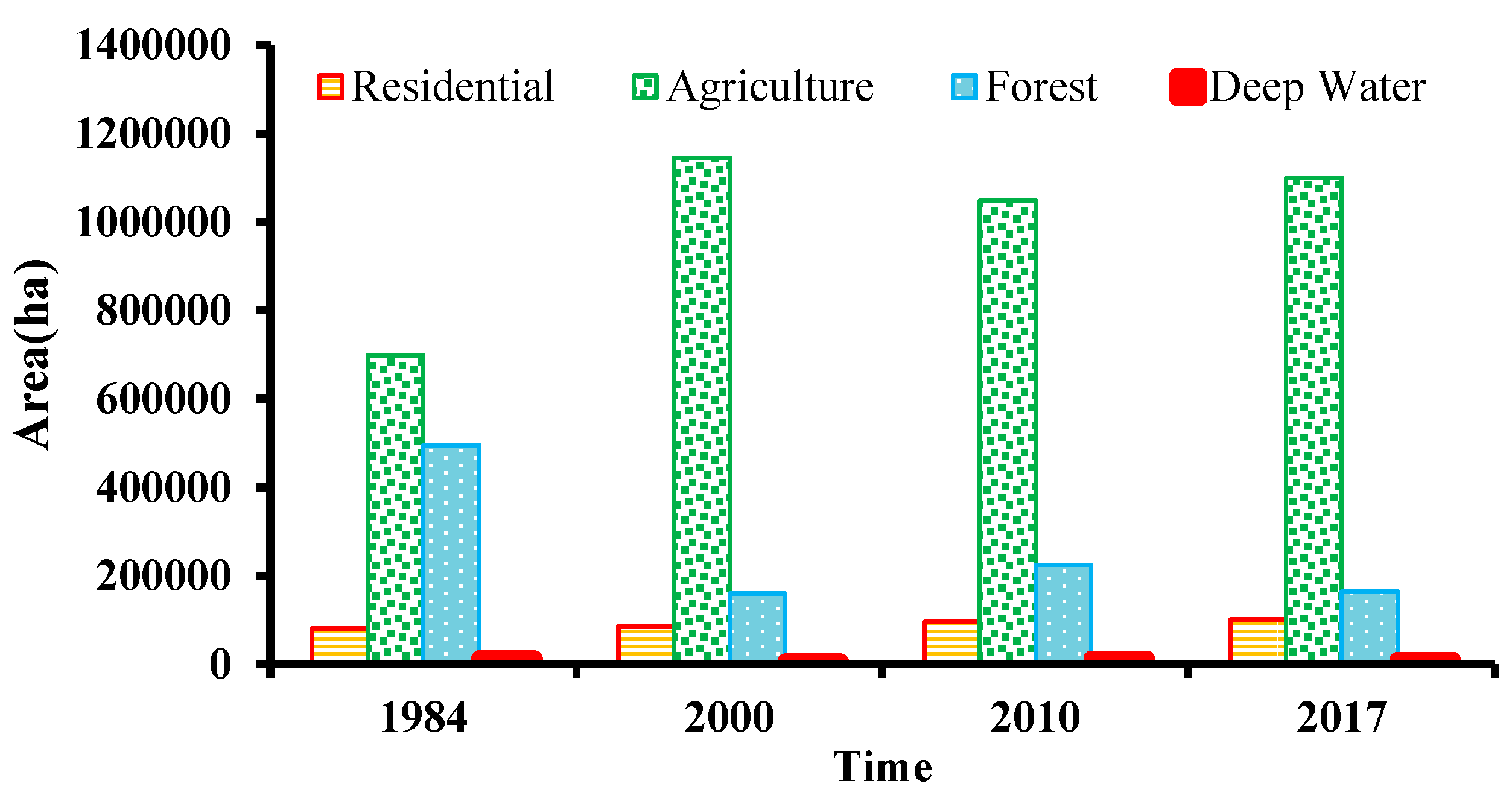
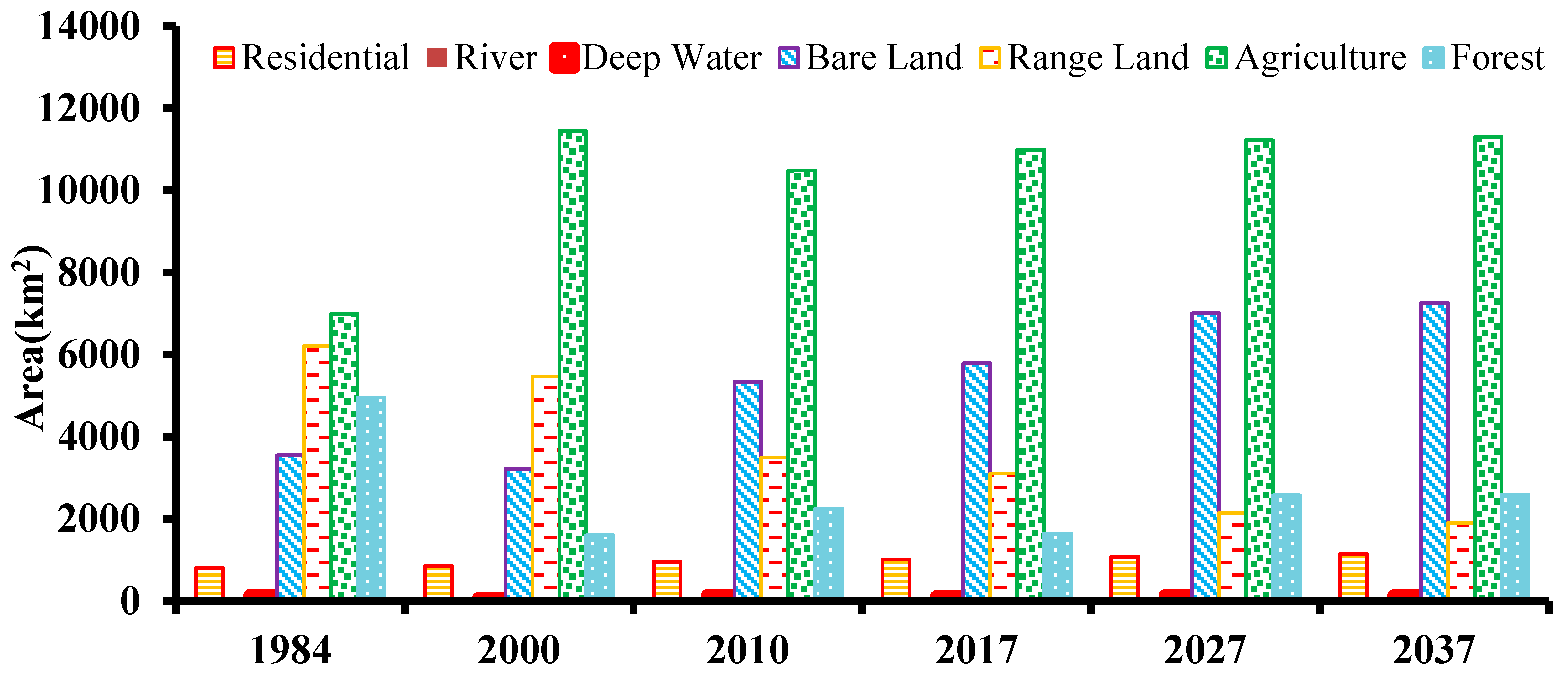
3.2. Anthropogenic LC Changes
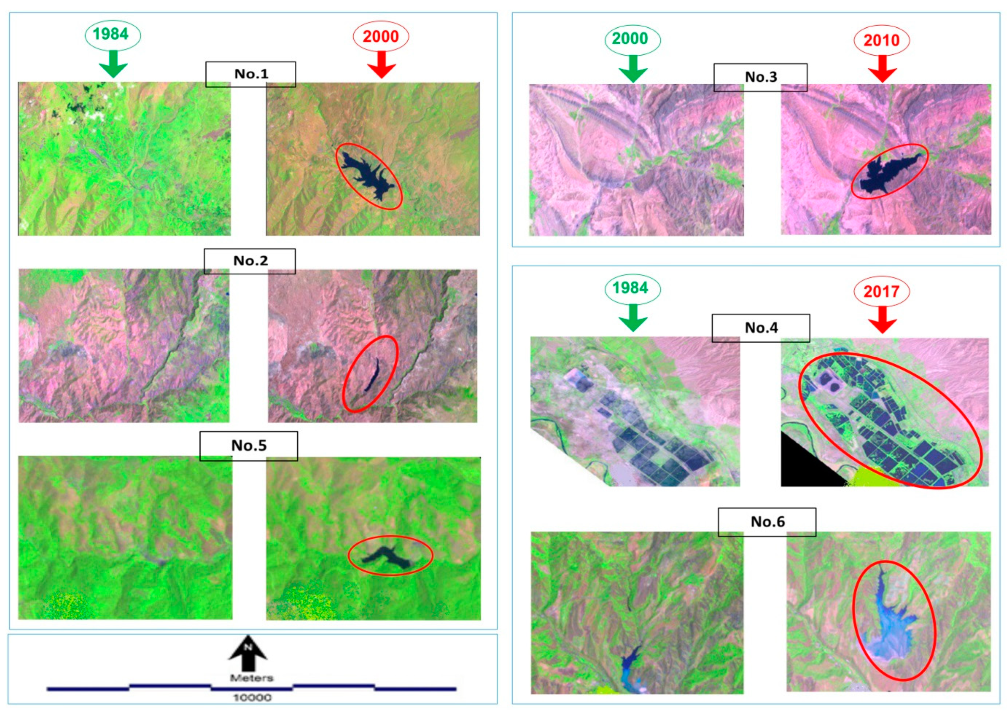
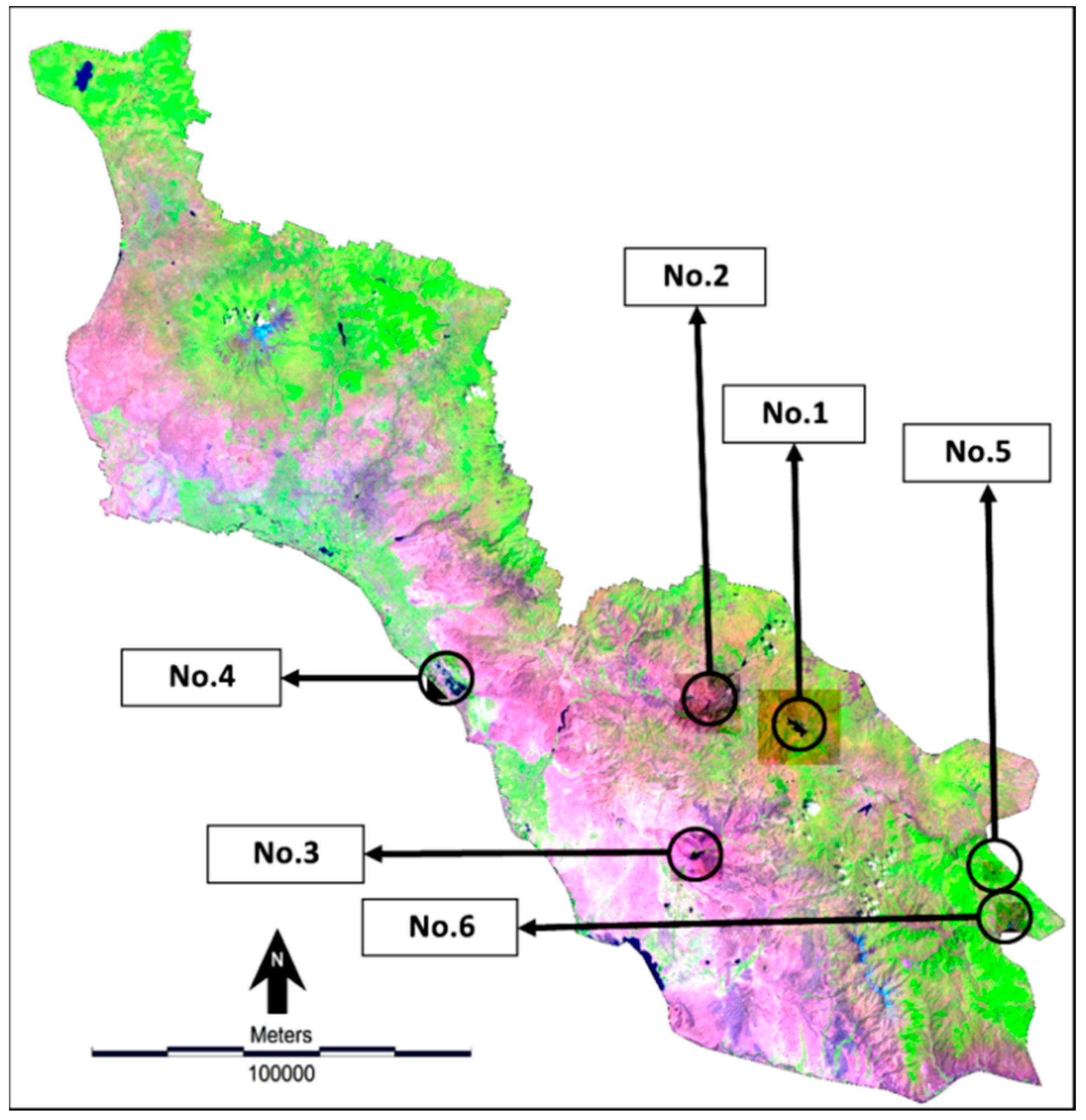
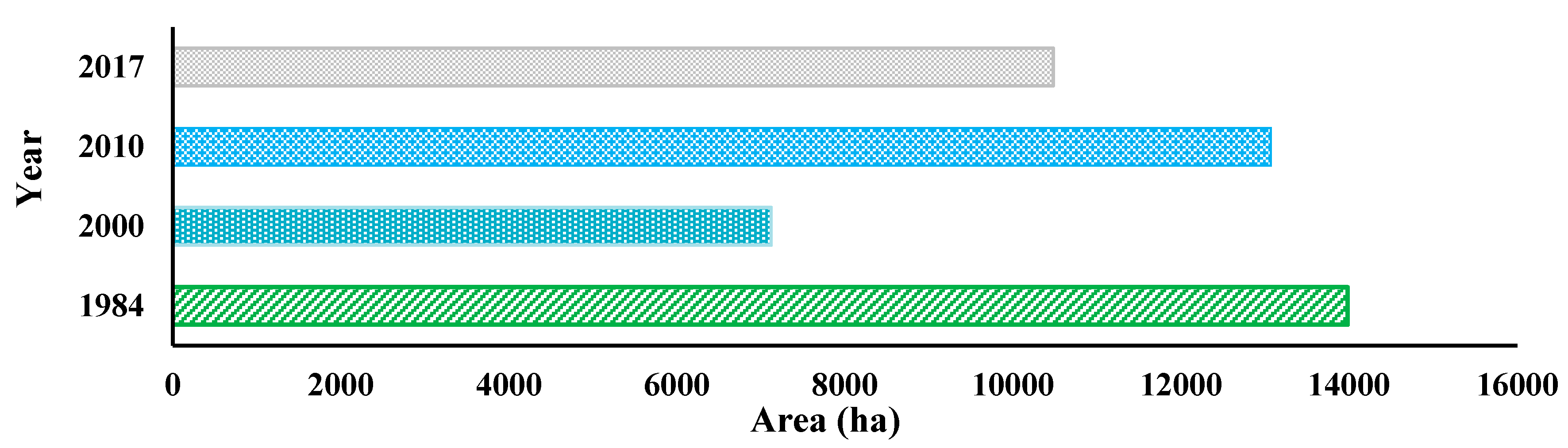
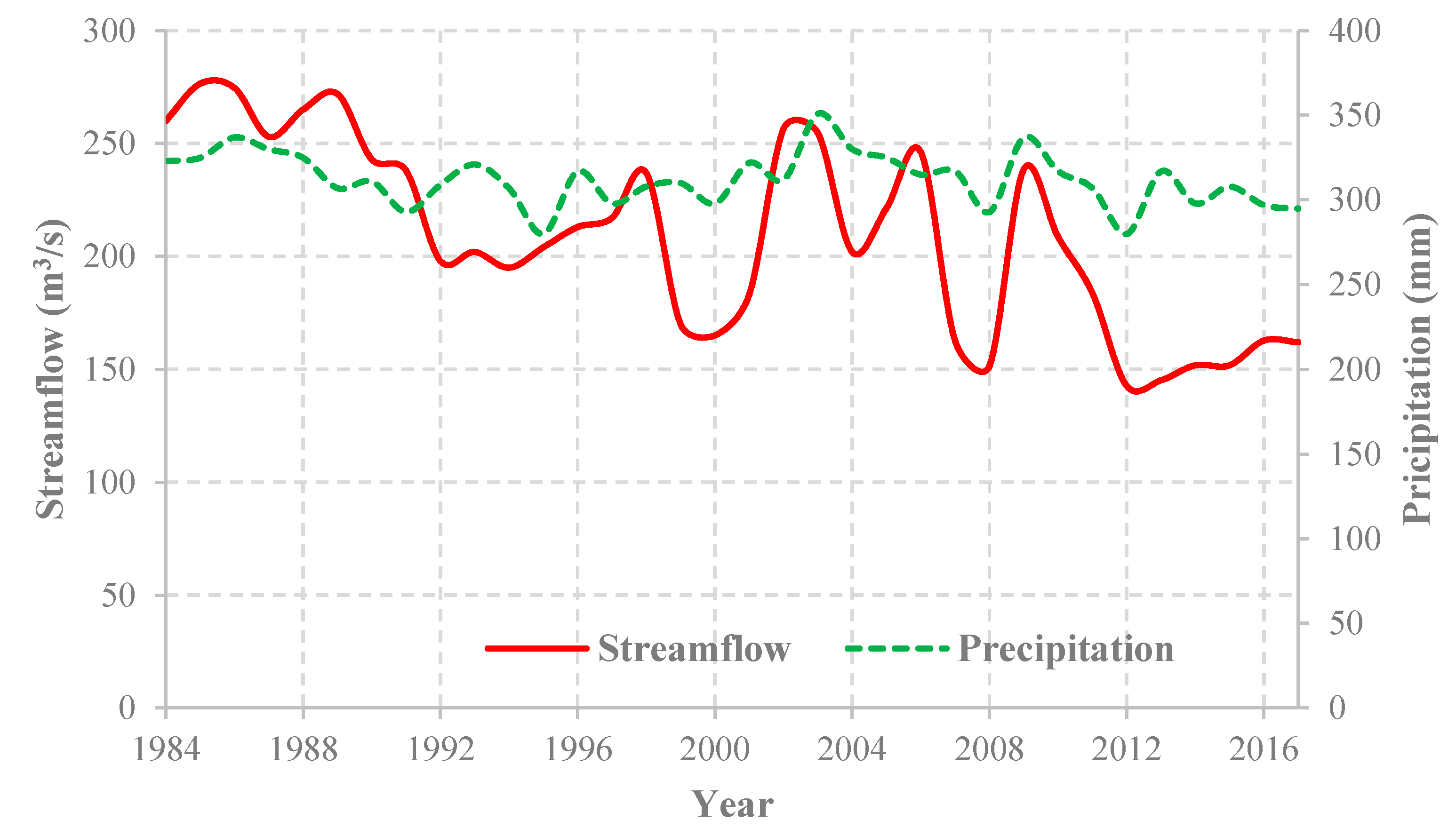
3.2.1. Changes in Water Bodies
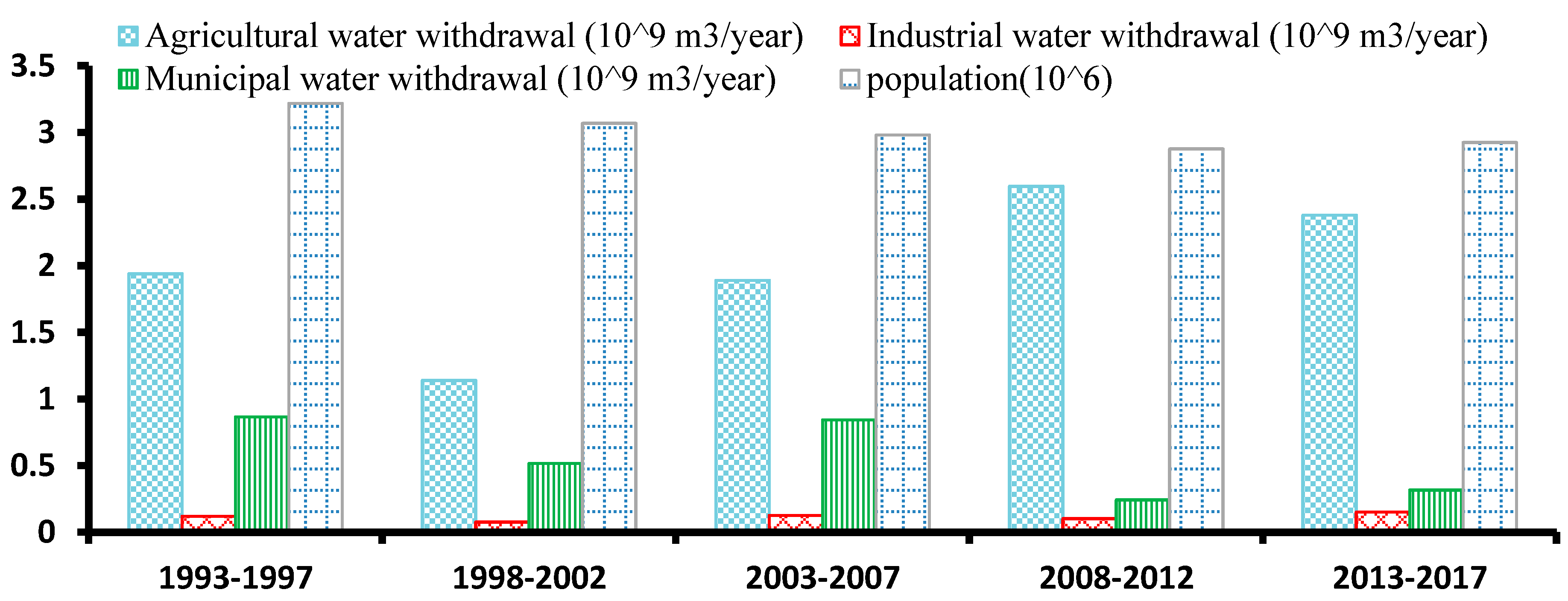
3.2.2. Changes in Agriculture, Forest, and Rangeland
3.3. LC Map Processing and Validation
3.4. Predicting Future LCs
4. Discussion
Limitations of the Study
5. Conclusions and Outlook
Author Contributions
Funding
Acknowledgments
Conflicts of Interest
References
- Yu, S.; Lu, H. Chemosphere Relationship between urbanisation and pollutant emissions in transboundary river basins under the strategy of the Belt and Road Initiative. Chemosphere 2018, 203, 11–20. [Google Scholar] [CrossRef] [PubMed]
- Castagna, J.; Calvello, M.; Esposito, F.; Pavese, G. Remote Sensing of Environment Analysis of equivalent black carbon multi-year data at an oil pre-treatment plant: Integration with satellite data to identify black carbon transboundary sources. Remote Sens. Environ. 2019, 235, 111429. [Google Scholar] [CrossRef]
- UNEP. Transboundary River Basins Status and Trends. In River Basins; Available online: http://www.geftwap.org/publications/river-basins-spm (accessed on 7 September 2020).
- Munia, H.; Guillaume, J.H.A.; Mirumachi, N.; Porkka, M.; Wada, Y.; Kummu, M. Water stress in global transboundary river basins: Significance of upstream water use on downstream stress. Environ. Res Lett. 2016, 11, 014002. [Google Scholar]
- De Stefano, L.; Duncan, J.; Dinar, S.; Stahl, K.; Strzepek, K.M.; Wolf, A.T. Climate change and the institutional resilience of international river basins. Peace Res. 2012, 49, 193–209. [Google Scholar] [CrossRef] [Green Version]
- Degefu, D.M.; He, W.; Yuan, L.; Zhao, J.H. Water Allocation in Transboundary River Basins under Water Scarcity: A Cooperative Bargaining Approach. Water Resour. Manag. 2016, 30, 4451–4466. [Google Scholar] [CrossRef]
- Konkoly-gyuró, É. Land Use Policy Conceptualisation and perception of the landscape and its changes in a transboundary area. A case study of the Southern German-French borderland. Land Use Policy 2018, 79, 556–574. [Google Scholar] [CrossRef]
- Mattsson, B.J.; Arih, A.; Heurich, M.; Santi, S.; Štemberk, J.; Vacik, H. Land Use Policy Evaluating a collaborative decision-analytic approach to inform conservation decision-making in transboundary regions. Land Use Policy 2019, 83, 282–296. [Google Scholar] [CrossRef]
- Ly, K.; Metternicht, G.; Marshall, L. Journal of Hydrology: Regional Studies Transboundary river catchment areas of developing countries: Potential and limitations of watershed models for the simulation of sediment and nutrient loads. A review. J. Hydrol. Reg. Stud. 2019, 24, 100605. [Google Scholar] [CrossRef]
- Mianabadi, H.; Mostert, E.; Pande, S. Weighted Bankruptcy Rules and Transboundary Water Resources Allocation. Water Resource Manag. 2015, 29, 2303–2321. [Google Scholar] [CrossRef] [Green Version]
- Guzha, A.C.; Rufino, M.C.; Okoth, S.; Jacobs, S.; Nóbrega, R.L.B. Impacts of land use and land cover change on surface runoff, discharge and low flows: Evidence from East Africa. J. Hydrol. Reg. Stud. 2018, 15, 49–67. [Google Scholar] [CrossRef]
- Younis, S.M.Z.; Ammar, A. Quantification of impact of changes in land use-land cover on hydrology in the upper Indus Basin, Pakistan. Egypt. J. Remote Sens. Space Sci. 2018, 21, 255–263. [Google Scholar] [CrossRef]
- Quyen, N.T.N.; Liem, N.D.; Loi, N.K. Effect of land use change on water discharge in Srepok watershed, Central Highland, Viet Nam. Int. Soil Water Conserv. Res. 2014, 2, 74–86. [Google Scholar] [CrossRef] [Green Version]
- Cuo, L.; Zhang, Y.; Gao, Y.; Hao, Z.; Cairang, L. The impacts of climate change and land cover/use transition on the hydrology in the upper Yellow River Basin, China. J. Hydrol. 2013, 502, 37–52. [Google Scholar] [CrossRef]
- Rahman, M.; Howladar, M.F.; Hossain, A.; Muzemder, A.T.M.S.H.; Numanbakth, A. Al Impact assessment of anthropogenic activities on water environment of Tillai River and its surroundings, Barapukuria Thermal Power Plant, Dinajpur, Bangladesh. Groundw. Sustain. Dev. 2019, 100310. [Google Scholar] [CrossRef]
- Mallinis, G.; Koutsias, N.; Arianoutsou, M. Science of the Total Environment Monitoring land use / land cover transformations from 1945 to 2007 in two peri-urban mountainous areas of Athens metropolitan area, Greece. Sci. Total Environ. 2014, 490, 262–278. [Google Scholar] [CrossRef]
- Gudmundsson, L.; Leonard, M.; Do, H.X.; Westra, S.; Seneviratne, S.I. Observed Trends in Global Indicators of Mean and Extreme Streamflow. Geophys. Res. Lett. 2019, 46, 756–766. [Google Scholar] [CrossRef] [Green Version]
- Ritchie, H.; Roser, M. Water Use and Stress. Available online: https://ourworldindata.org/water-use-stress (accessed on 9 October 2020).
- Sharma, P.J.; Patel, P.L.; Jothiprakash, V. Impact of rainfall variability and anthropogenic activities on stream fl ow changes and water stress conditions across Tapi Basin in India. Sci. Total Environ. 2019, 687, 885–897. [Google Scholar] [CrossRef]
- Kuenzer, C.; Campbell, I.; Roch, M.; Leinenkugel, P.; Quoc, V.; Stefan, T. Understanding the impact of hydropower developments in the context of upstream—Downstream relations in the Mekong river basin. Sustain. Sci. 2012, 8, 565–584. [Google Scholar] [CrossRef]
- Yang, J.; Yang, Y.C.E.; Chang, J.; Zhang, J.; Yao, J. Impact of Dam Development and Climate Change on Hydroecological Conditions and Natural Hazard Risk in the Mekong River Basin. J. Hydrol. 2019. [Google Scholar] [CrossRef]
- Nugroho, P.; Marsono, D.; Sudira, P.; Suryatmojo, H. The 3 rd International Conference on Sustainable Future for Human Security Impact of land-use changes on water balance. Procedia Environ. Sci. 2013, 17, 256–262. [Google Scholar] [CrossRef] [Green Version]
- Deng, X.; Shi, Q.; Zhang, Q.; Shi, C.; Yin, F. Impacts of land use and land cover changes on surface energy and water balance in the Heihe River Basin of China, 2000–2010. J. Phys. Chem. EAR 2015, 2000–2010. [Google Scholar] [CrossRef]
- Sun, Z.; Wu, F.; Shi, C.; Zhan, J. The impact of land use change on water balance in Zhangye city, China. Phys. Chem. Earth 2016. [Google Scholar] [CrossRef]
- Gao, J.; Li, F.; Gao, H.; Zhou, C.; Zhang, X. The impact of land-use change on water-related ecosystem services: A study of the Guishui River Basin, Beijing, China. J. Clean. Prod. 2017, 163, S148–S155. [Google Scholar] [CrossRef]
- Lang, Y.; Song, W.; Deng, X. Projected land use changes impacts on water yields in the karst mountain areas of China. Phys. Chem. Earth 2018, 104, 66–75. [Google Scholar] [CrossRef]
- Ferreira, P.; Van Soesbergen, A.; Mulligan, M.; Freitas, M.; Vale, M.M. Can forests buffer negative impacts of land-use and climate changes on water ecosystem services? The case of a Brazilian megalopolis. Sci. Total Environ. 2019, 685, 248–258. [Google Scholar] [CrossRef]
- Giri, S.; Arbab, N.N.; Lathrop, R.G. Assessing the potential impacts of climate and land use change on water fl uxes and sediment transport in a loosely coupled system. J. Hydrol. 2019, 577, 123955. [Google Scholar] [CrossRef]
- Shrestha, S.; Bhatta, B.; Shrestha, M.; Shrestha, P.K. assessment of the climate and landuse change impact on hydrology and water quality in the Songkhram River Basin, Thailand. Sci. Total Environ. 2018, 643, 1610–1622. [Google Scholar] [CrossRef]
- Amjath-babu, T.S.; Sharma, B.; Brouwer, R.; Rasul, G.; Wahid, S.M.; Neupane, N.; Bhattarai, U.; Sieber, S. Integrated modelling of the impacts of hydropower projects on the water- food-energy nexus in a transboundary Himalayan river basin. Appl. Energy 2019, 239, 494–503. [Google Scholar] [CrossRef]
- Jin-song, D.; Ke, W.; Jun, L.; Yan-hua, D. Urban Land Use Change Detection Using Multisensor Satellite Images. Pedosphere 2009, 19, 96–103. [Google Scholar] [CrossRef]
- Rogan, J.; Chen, D. Remote sensing technology for mapping and monitoring land-cover and land-use change. Prog. Plan. 2004, 61, 301–325. [Google Scholar] [CrossRef]
- Roy, D.P.; Wulder, M.A.; Loveland, T.R.; Woodcock, C.E.; Allen, R.G.; Anderson, M.C.; Helder, D.; Irons, J.R.; Johnson, D.M.; Kennedy, R.; et al. Remote Sensing of Environment Landsat-8: Science and product vision for terrestrial global change research. Remote Sens. Environ. 2014, 145, 154–172. [Google Scholar] [CrossRef] [Green Version]
- Li, X.; Zhou, Y. A national dataset of 30-m annual urban extent dynamics (1985–2015) in the conterminous United States. Earth Syst. Sci. Data 2020, 12, 357–371. [Google Scholar] [CrossRef] [Green Version]
- Shang, R.; Zhu, Z. Remote Sensing of Environment Harmonizing Landsat 8 and Sentinel-2: A time-series-based re fl ectance adjustment approach. Remote Sens. Environ. 2019, 235, 111439. [Google Scholar] [CrossRef]
- Heidari, A. Aras transboundary river basin cooperation perspective Aras transboundary river basin cooperation perspective. In Proceedings of the Commission on Large Dams 79th Annual Meeting, Lucerne, Switzerland, 1 June 2011. [Google Scholar]
- FAO. Kura-Araks River Basin, Irrigation in the Middle East Region in Tabures—AQUASTAT Survey; FAO: Rome, Italy, 2008; pp. 1–6. [Google Scholar]
- Nasehi, F.; Hassani, A.; Monavvari, M.; Karbassi, A.; Khorasani, N.; Imani, A. Heavy Metal Distributions in Water of the Aras River. J. Water Resource Protect. 2012, 2012, 73–78. [Google Scholar] [CrossRef] [Green Version]
- Nasrabadi, T.; Nabi, R.; Karbassi, A.R.; Pezeshk, H. Influence of Sungun copper mine on groundwater quality, NW Iran Influence of Sungun copper mine on groundwater quality. Environ. Geol. 2009, 58, 693–700. [Google Scholar] [CrossRef]
- Schneider, A. Monitoring land cover change in urban and peri-urban areas using dense time stacks of Landsat satellite data and a data mining approach. Remote Sens. Environ. 2012, 124, 689–704. [Google Scholar] [CrossRef]
- Clark, M.L.; Aide, T.M. Virtual interpretation of Earth Web-Interface Tool (VIEW-IT) for collecting land-use/land-cover reference data. Remote Sens. 2011, 3, 601–620. [Google Scholar] [CrossRef] [Green Version]
- Ahmed, K.R.; Akter, S. Analysis of landcover change in southwest Bengal delta due to floods by NDVI, NDWI and K-means cluster with landsat multi-spectral surface reflectance satellite data. Remote Sens. Appl. Soc. Environ. 2017, 8, 168–181. [Google Scholar] [CrossRef]
- Szabó, S.; Gácsi, Z.; Balázs, B. Specific features of NDVI, NDWI and MNDWI as reflected in land cover categories. Landsc. Environ. 2016, 10, 194–202. [Google Scholar] [CrossRef]
- Gandhi, G.M.; Parthiban, S.; Thummalu, N.; Christy, A. Ndvi: Vegetation Change Detection Using Remote Sensing and Gis—A Case Study of Vellore District. Procedia Comput. Sci. 2015, 57, 1199–1210. [Google Scholar] [CrossRef] [Green Version]
- Rawat, J.S.; Kumar, M. Monitoring land use/cover change using remote sensing and GIS techniques: A case study of Hawalbagh block, district Almora, Uttarakhand, India. Egypt. J. Remote Sens. Space Sci. 2015, 18, 77–84. [Google Scholar] [CrossRef] [Green Version]
- Chang, H.; Yoon, W.S. Improving the classification of Landsat data using standardized principal components analysis. KSCE J. Civ. Eng. 2003, 7, 469–474. [Google Scholar] [CrossRef]
- Thakkar, A.; Desai, V.; Patel, A.; Potdar, M. Land use/land cover classification using remote sensing data and derived indices in a heterogeneous landscape of a khan-kali watershed, Gujarat. Asian J. Geoinform. 2015, 14. [Google Scholar]
- Erbek, F.S.; Özkan, C.; Taberner, M. Comparison of maximum likelihood classification method with supervised artificial neural network algorithms for land use activities. Int. J. Remote Sens. 2004, 25, 1733–1748. [Google Scholar] [CrossRef]
- McFeeters, S.K. The use of the Normalized Difference Water Index (NDWI) in the delineation of open water features. Int. J. Remote Sens. 1996, 17, 1425–1432. [Google Scholar] [CrossRef]
- Acharya, T.D.; Subedi, A.; Lee, D. Evaluation of Water Indices for Surface Water Extraction in a Landsat 8 Scene of Nepal. Sensors 2018, 18, 2580. [Google Scholar] [CrossRef] [PubMed] [Green Version]
- Özelkan, E. Water body detection analysis using NDWI indices derived from landsat-8 OLI. Polish J. Environ. Stud. 2020, 29, 1759–1769. [Google Scholar] [CrossRef]
- Ji, L.; Zhang, L.; Wylie, B. Analysis of Dynamic Thresholds for the Normalized Difference Water Index. Photogramm. Eng. Remote Sens. 2009, 75, 1307–1317. [Google Scholar] [CrossRef]
- Liu, Z.; Yao, Z.; Wang, R. Assessing methods of identifying open water bodies using Landsat 8 OLI imagery. Environ. Earth Sci. 2016, 75, 1–13. [Google Scholar] [CrossRef]
- Mirzaei, A.; Saghafian, B.; Mirchi, A.; Madani, K. The Groundwater-Energy-Food Nexus in Iran’s Agricultural Sector: Implications for Water Security. Water 2019, 11, 1835. [Google Scholar]
- Stehman, S.V. Sampling designs for accuracy assessment of land cover. Int. J. Remote Sens. 2009, 30, 5243–5272. [Google Scholar] [CrossRef]
- Foody, G.M. Status of land cover classification accuracy assessment. Remote Sens. Environ. 2002, 80, 185–201. [Google Scholar] [CrossRef]
- McHugh, M.L. Lessons in biostatistics interrater reliability: The kappa statistic. Biochem. Med. 2012, 22, 276–282. [Google Scholar] [CrossRef]
- Viera, A.J.; Garrett, J.M. Understanding interobserver agreement: The kappa statistic. Fam. Med. 2005, 37, 360–363. [Google Scholar]
- Pontius, R.G. Quantification error versus location error in comparison of categorical maps. Photogramm. Eng. Remote Sens. 2000, 66, 1011–1016. [Google Scholar]
- Eastman, J.R. IDRISI Andes; Guide to GIS and Image Processing; Clark Labs, Clark University: Worcester, MA, USA, 2006. [Google Scholar]
- Razavi, S.; Tolson, B.; Burn, D.; Seglenieks, F. Reformulated Neural Network (ReNN): A New Alternative for Data-driven Modelling in Hydrology and Water Resources Engineering. IEEE Trans. Neural Netw. 2011, 22, 1588–1898. [Google Scholar] [CrossRef]
- Japelaghi, M.; Gholamalifard, M.; Shayesteh, K. Spatio-temporal analysis and prediction of landscape patterns and change processes in the Central Zagros region, Iran. Remote Sens. Appl. Soc. Environ. 2019, 15, 100244. [Google Scholar] [CrossRef]
- Linkie, M.; Smith, R.J.; Leader-Williams, N. Mapping and predicting deforestation patterns in the lowlands of Sumatra. Biodivers. Conserv. 2004, 13, 1809–1818. [Google Scholar] [CrossRef]
- Schulz, J.J.; Cayuela, L.; Echeverria, C.; Salas, J.; Rey Benayas, J.M. Monitoring land cover change of the dryland forest landscape of Central Chile (1975–2008). Appl. Geogr. 2010, 30, 436–447. [Google Scholar] [CrossRef] [Green Version]
- Pistocchi, A.; Luzi, L.; Napolitano, P. The use of predictive modeling techniques for optimal exploitation of spatial databases: A case study in landslide hazard mapping with expert system-like methods. Environ. Geol. 2002, 41, 765–775. [Google Scholar] [CrossRef]
- Takada, T.; Miyamoto, A.; Hasegawa, S.F. Derivation of a yearly transition probability matrix for land-use dynamics and its applications. Landsc. Ecol. 2010, 25, 561–572. [Google Scholar] [CrossRef]
- Eastman, J.R.; Toledano, J. A Short Presentation of the Land Change Modeler (LCM). In Geomatic Approaches for Modeling Land Change Scenarios; Springer: Cham, Switzerland, 2018; pp. 499–505. ISBN 9783319608013. [Google Scholar]
- Pérez-Vega, A.; Mas, J.F.; Ligmann-Zielinska, A. Comparing two approaches to land use/cover change modeling and their implications for the assessment of biodiversity loss in a deciduous tropical forest. Environ. Model. Softw. 2012, 29, 11–23. [Google Scholar] [CrossRef]
- Khoi, D.D.; Murayama, Y. Forecasting areas vulnerable to forest conversion in the tam Dao National Park region, Vietnam. Remote Sens. 2010, 2, 1249–1272. [Google Scholar] [CrossRef] [Green Version]
- Oñate-Valdivieso, F.; Bosque Sendra, J. Application of GIS and remote sensing techniques in generation of land use scenarios for hydrological modeling. J. Hydrol. 2010, 395, 256–263. [Google Scholar] [CrossRef]
- Foley, J.A.; Defries, R.; Asner, G.P.; Barford, C.; Bonan, G.; Carpenter, S.R.; Chapin, F.S.; Coe, M.T.; Daily, G.C.; Gibbs, H.K.; et al. Global Consequences of Land Use. Science 2005, 309, 570–575. [Google Scholar] [CrossRef] [PubMed] [Green Version]
- Zhao, S.; Peng, C.; Jiang, H.; Tian, D.; Lei, X.; Zhou, X. Land use change in Asia and the ecological consequences. Ecol. Res. 2006, 21, 890–896. [Google Scholar] [CrossRef]
- Fang, J.; Rao, S.; Zhao, S. Human-induced long-term changes in the lakes of the Jianghan Plain, Central Yangtze. Front. Ecol. Environ. 2005, 3, 186–192. [Google Scholar] [CrossRef]
- Castelletta, M.; Sodhi, N.S.; Subaraj, R. Heavy Extinctions of Forest Avifauna in Singapore: Lessons for Biodiversity Conservation in Southeast Asia. Conserv. Biol. 2000, 14, 1870–1880. [Google Scholar] [CrossRef]
- Hillstrom, K.; Hillstrom, L.C. North America: A Continental Overview of Environmental Issues; ABC-CLIO: Denver, CO, USA; Oxford, UK, 2003. [Google Scholar]
- Hajihosseini, M.; Hajihosseini, H.; Morid, S.; Delavar, M.; Booij, M.J. Impacts of land use changes and climate variability on transboundary Hirmand River using SWAT. J. Water Clim. Chang. 2019, 1–18. [Google Scholar] [CrossRef]
- Al-Saady, Y.; Merkel, B.; Al-Tawash, B.; Al-Suhail, Q. Land use and land cover (LULC) mapping and change detection in the Little Zab River Basin (LZRB), Kurdistan Region, NE Iraq and NW Iran. FOG Freib. Online Geosci. 2015, 43, 1–32. [Google Scholar]
- Dudgeon, D. Endangered ecosystems: A review of the conservation status of tropical Asian rivers. Hydrobiologia 1992, 248, 167–191. [Google Scholar]
- Kumar, A.; Kanaujia, A. Wetlands: Significance, Threats and their Conservation. Dir. Environ. 2014, 7, 1–24. [Google Scholar]
- Moreno-Sanchez, R.; Sayadyan, H.; Streeter, R.; Rozelle, J. The Armenian forests: Threats to conservation and needs for sustainable management. Ecosyst. Sustain. Dev. 2007, 106, 113–122. [Google Scholar] [CrossRef] [Green Version]
- HOUGHTON, R.A.; HACKLER, J.L. Emissions of carbon from forestry and land-use change in tropical Asia. Glob. Chang. Biol. 1999, 5, 481–492. [Google Scholar] [CrossRef]
- Ogutu, J.O.; Piepho, H.P.; Dublin, H.T.; Bhola, N.; Reid, R.S. Dynamics of Mara-Serengeti ungulates in relation to land use changes. J. Zool. 2009, 278, 1–14. [Google Scholar] [CrossRef]
- Kiragu, G.M. Assessment of Suspended Sediment Loadings and Their Impact on the Environmental Flows of Upper Transboundary Mara River, Kenya. Master’s Thesis, Jomo Kenyatta University of Agriculture and Technology, Juya, Kenya, 2009. [Google Scholar]
- FAO. AQUASTAT Database. Available online: http://www.fao.org/nr/water/aquastat/data/query/index.html?lang=en (accessed on 7 January 2020).
- Bank, W. The Republic of Armenia, Climate Change and Agriculture Country Note; World Bank: Washington, DC, USA, 2012; p. 21. [Google Scholar]
- Aubrey, D.G. Reducing Transboundary Degradation in the Kura-Aras River Basin Final Terminal Evaluation Report. Available online: https://iwlearn.net/resolveuid/5ed0f3514f4447f4703162c0ca76b1c1 (accessed on 18 September 2020).
- Barannik, V.; Borysova, O.; Stolberg, F. The Caspian Sea Region: Environmental Change. AMBIO A J. Hum. Environ. 2004, 33, 45–51. [Google Scholar] [CrossRef]
- Mwangi, H.M.; Julich, S.; Patil, S.D.; McDonald, M.A.; Feger, K.H. Relative contribution of land use change and climate variability on discharge of upper Mara River, Kenya. J. Hydrol. Reg. Stud. 2016, 5, 244–260. [Google Scholar] [CrossRef] [Green Version]


| Data | Source | Date | Objective/Description |
|---|---|---|---|
| Digital elevation model (DEM) | ASTER | 2014 | Used for modeling/Spatial resolution of 30 m |
| Infrastructure maps | OSM database | 2011 | Used to produce LC maps and extract road layers and natural zones |
| DIVA GIS | - | Include roads, rivers, political zones | |
| World watershed database | - | Zoning of basins | |
| Landsat images | Landsat 5 TM | 1983/07/10 | Used to produce LC maps |
| 1984/07/07 | Used to produce LC maps | ||
| 1984/07/23 | Used to produce LC maps | ||
| 1985/07/27 | Used to produce LC maps | ||
| Landsat 7 ETM | 2000/07/29 | Used to produce LC maps | |
| 2000/07/22 | Used to produce LC maps | ||
| 2000/07/22 | Used to produce LC maps | ||
| 1999/06/13 | Used to produce LC maps | ||
| Landsat 7 TM+ | 2010/07/10 | Used to produce LC maps | |
| 2010/07/28 | Used to produce LC maps | ||
| 2010/07/28 | Used to produce LC maps | ||
| 2009/06/27 | Used to produce LC maps | ||
| Landsat 8 OLI | 2017/07/28 | Used to produce LC maps | |
| 2017/07/28 | Used to produce LC maps | ||
| 2017/07/05 | Used to produce LC maps | ||
| 2017/06/03 | Used to produce LC maps | ||
| Google Earth images | Historical images | Accuracy assessment and correction | |
| Scenario Code | Scenario Name | Sub-Model | Input Variables | Prediction for Year | Reference Map for Validation |
|---|---|---|---|---|---|
| 1 | Forest to agriculture | A | DEM map | 2010 2017 And 2027 | Generated LC map in 2010 Generated LC map in 2027 None |
| Distance from bare land in 1984 | |||||
| Distance from agriculture in 1984 | |||||
| Distance from forest in 1984 | |||||
| Distance from residential areas in 1984 | |||||
| Distance from river in 1984 | |||||
| 2 | Agriculture to rangeland | B | DEM map | 2010 2017 And 2027 | Generated LC map in 2010 Generated LC map in 2027 None |
| Distance from bare land in 1984 | |||||
| Distance from agriculture in 1984 | |||||
| Distance from forest in 1984 | |||||
| Qualitative variables in rangeland | |||||
| 3 | Bare land to rangeland | C | Distance from forest in 1984 | 2010 2017 And 2027 | Generated LC map in 2010 Generated LC map in 2027 None |
| Distance from agriculture in 1984 | |||||
| Distance from residential areas in 1984 | |||||
| Qualitative variables in rangeland | |||||
| 4 | Rangeland to agriculture | D | DEM map | 2010 2017 And 2027 | Generated LC map in 2010 Generated LC map in 2027 None |
| Distance from bare land in 1984 | |||||
| Distance from agriculture in 1984 | |||||
| Distance from forest in 1984 | |||||
| Distance from residential areas in 1984 | |||||
| 5 | All transmission sub-models | E | DEM map | 2010 2017 And 2027 | Generated LC map in 2010 Generated LC map in 2027 None |
| Distance from river in 1984 | |||||
| Distance from agriculture in 1984 | |||||
| Distance from bare land in 1984 | |||||
| Distance from residential areas in 1984 | |||||
| Distance from rangeland in 1984 | |||||
| Distance from forest in 1984 | |||||
| Qualitative variables in all sub-models |
| Scenario Code | Scenario Name | Sub-Model | Input Variables | Prediction for Year | Reference Map for Validation |
|---|---|---|---|---|---|
| 1 | Agriculture to forest | A | DEM map | 2017 2027 And 2037 | Generated LC map in 2017 None None |
| Distance from bare land in 2000 | |||||
| Distance from agriculture in 2000 | |||||
| Distance from forest in 2000 | |||||
| Qualitative variables in forest | |||||
| 2 | Agriculture to rangeland | B | DEM map | 2017 2027 And 2037 | Generated LC map in 2017 None None |
| Distance from bare land in 2000 | |||||
| Distance from agriculture in 2000 | |||||
| Distance from forest in 2000 | |||||
| Qualitative variables in rangeland | |||||
| 3 | forest to agriculture | C | DEM map | 2017 2027 And 2037 | Generated LC map in 2017 None None |
| Distance from bare land in 2000 | |||||
| Distance from agriculture in 2000 | |||||
| Distance from forest in 2000 | |||||
| Qualitative variables in agriculture | |||||
| 4 | Rangeland to agriculture | D | DEM map | 2017 2027 And 2037 | Generated LC map in 2017 None None |
| Distance from bare land in 2000 | |||||
| Distance from agriculture in 2000 | |||||
| Distance from forest in 2000 | |||||
| Qualitative variables in agriculture | |||||
| 5 | Rangeland to bare land | E | DEM map | 2017 2027 And 2037 | Generated LC map in 2017 None None |
| Distance from bare land in 2000 | |||||
| Distance from agriculture in 2000 | |||||
| Distance from forest in 2000 | |||||
| Qualitative variables in bare land | |||||
| 6 | All transmission sub-models | F | DEM map | 2017 2027 And 2037 | Generated LC map in 2017 None None |
| Distance from bare land in 2000 | |||||
| Distance from agriculture in 2000 | |||||
| Distance from forest in 2000 | |||||
| Distance from rangeland in 2000 | |||||
| Qualitative variables in all sub-models |
| Forest | Agriculture | Rangelands | Bare Lands | Deep Water | River | Residential | Overall Kappa | |
|---|---|---|---|---|---|---|---|---|
| LC map 1984 | 0.80 | 0.75 | 0.82 | 0.92 | 0.96 | 0.83 | 0.99 | 0.87 |
| LC map 2000 | 0.79 | 0.78 | 0.84 | 0.90 | 0.97 | 0.86 | 0.98 | 0.87 |
| LC map 2010 | 0.83 | 0.72 | 0.79 | 0.88 | 0.94 | 0.81 | 0.96 | 0.85 |
| LC map 2017 | 0.89 | 0.74 | 0.81 | 0.94 | 0.98 | 0.78 | 0.99 | 0.88 |
| Number of Dams | Country | Coordinates (meters) | Area (hectares) | Construction Period | Description |
|---|---|---|---|---|---|
| 1 | Armenia | X: 570211 Y: 4390210 | 724.5 | 1984–2000 | Concrete dam built to store water |
| 2 | Armenia | X: 546876 Y: 4396219 | 98.37 | 1984–2000 | Embankment dam built to store water for irrigation |
| 3 | Nakhchivan | X: 543572 Y: 4359306 | 283 | 2000–2010 | Concrete dam built to store water and generate power |
| 4 | Armenia | X: 479771 Y: 4402030 | 1403 | 1984–2017 | Aquaculture production |
| 5 | Armenia | X: 621165 Y: 4355374 | 17 | 1984–2000 | Soil dam for water storage and infiltration |
| 6 | Armenia | X: 625851 Y: 4344088 | 299 | 1984–2017 | Soil dam built for water storage and feed agriculture |
| Variables | DEM | Aspect | Slope | Distance from Rangeland | Distance from Roads | Distance from River | Distance from Agriculture | Distance from Bare Land | Distance from Deep Water | Distance from Residential Areas |
|---|---|---|---|---|---|---|---|---|---|---|
| Overall Cramer’s V | 0.214 | 0.131 | 0.129 | 0.171 | 0.023 | 0.034 | 0.164 | 0.129 | 0.197 | 0.231 |
| Rangeland | 0.182 | 0.067 | 0.154 | 0.213 | 0.078 | 0.046 | 0.324 | 0.289 | 0.138 | 0.074 |
| Bare land | 0.158 | 0.040 | 0.124 | 0.142 | 0.041 | 0.087 | 0.143 | 0.129 | 0.174 | 0.057 |
| Agriculture | 0.141 | 0.084 | 0.041 | 0.112 | 0.034 | 0.068 | 0.071 | 0.176 | 0.143 | 0.043 |
| Residential areas | 0.02 | 0.027 | 0.039 | 0.023 | 0.042 | 0.097 | 0.017 | 0.132 | 0.041 | 0.084 |
| Rivers | 0.174 | 0.128 | 0.302 | 0.228 | 0.038 | 0.047 | 0.238 | 0.154 | 0.487 | 0.045 |
| Deep water | 0.413 | 0.056 | 0.079 | 0.143 | 0.072 | 0.079 | 0.359 | 0.402 | 0.184 | 0.137 |
| Forests | 0.002 | 0.000 | 0.021 | 0.012 | 0.000 | 0.014 | 0.000 | 0.012 | 0.009 | 0.001 |
© 2020 by the authors. Licensee MDPI, Basel, Switzerland. This article is an open access article distributed under the terms and conditions of the Creative Commons Attribution (CC BY) license (http://creativecommons.org/licenses/by/4.0/).
Share and Cite
Khoshnoodmotlagh, S.; Verrelst, J.; Daneshi, A.; Mirzaei, M.; Azadi, H.; Haghighi, M.; Hatamimanesh, M.; Marofi, S. Transboundary Basins Need More Attention: Anthropogenic Impacts on Land Cover Changes in Aras River Basin, Monitoring and Prediction. Remote Sens. 2020, 12, 3329. https://doi.org/10.3390/rs12203329
Khoshnoodmotlagh S, Verrelst J, Daneshi A, Mirzaei M, Azadi H, Haghighi M, Hatamimanesh M, Marofi S. Transboundary Basins Need More Attention: Anthropogenic Impacts on Land Cover Changes in Aras River Basin, Monitoring and Prediction. Remote Sensing. 2020; 12(20):3329. https://doi.org/10.3390/rs12203329
Chicago/Turabian StyleKhoshnoodmotlagh, Sajad, Jochem Verrelst, Alireza Daneshi, Mohsen Mirzaei, Hossein Azadi, Mohammad Haghighi, Masoud Hatamimanesh, and Safar Marofi. 2020. "Transboundary Basins Need More Attention: Anthropogenic Impacts on Land Cover Changes in Aras River Basin, Monitoring and Prediction" Remote Sensing 12, no. 20: 3329. https://doi.org/10.3390/rs12203329
APA StyleKhoshnoodmotlagh, S., Verrelst, J., Daneshi, A., Mirzaei, M., Azadi, H., Haghighi, M., Hatamimanesh, M., & Marofi, S. (2020). Transboundary Basins Need More Attention: Anthropogenic Impacts on Land Cover Changes in Aras River Basin, Monitoring and Prediction. Remote Sensing, 12(20), 3329. https://doi.org/10.3390/rs12203329