Article

Dissolved Oxygen Forecasting in Aquaculture: A Hybrid Model Approach

Institute for Research in Applicable Computing (IRAC), School of Computer Science and Technology, University of Bedfordshire, Luton LU1 3JU, UK
*
Author to whom correspondence should be addressed.
Appl. Sci. 2020, 10(20), 7079; https://doi.org/10.3390/app10207079
Submission received: 21 September 2020 / Revised: 3 October 2020 / Accepted: 6 October 2020 / Published: 12 October 2020
(This article belongs to the Special Issue Newly Sensors and Biosensors for Water Quality Monitoring)

Abstract

:
Dissolved oxygen (DO) concentration is a vital parameter that indicates water quality. We present here DO short term forecasting using time series analysis on data collected from an aquaculture pond. This can provide the basis of data support for an early warning system, for an improved management of the aquaculture farm. The conventional forecasting approaches are commonly characterized by low accuracy and poor generalization problems. In this article, we present a novel hybrid DO concentration forecasting method with ensemble empirical mode decomposition (EEMD)-based LSTM (long short-term memory) neural network (NN). With this method, first, the sensor data integrity is improved through linear interpolation and moving average filtering methods of data preprocessing. Next, the EEMD algorithm is applied to decompose the original sensor data into multiple intrinsic mode functions (IMFs). Finally, the feature selection is used to carefully select IMFs that strongly correlate with the original sensor data, and integrate into both inputs for the NN. The hybrid EEMD-based LSTM forecasting model is then constructed. The performance of this proposed model in training and validation sets was compared with the observed real sensor data. To obtain the exact evaluation accuracy of the forecasted results of the hybrid EEMD-based LSTM forecasting model, four statistical performance indices were adopted: mean absolute error (MAE), mean square error (MSE), root mean square error (RMSE), and mean absolute percentage error (MAPE). Results are presented for the short term (12-h) and the long term (1-month) that are encouraging, indicating suitability of this technique for forecasting DO values.

1. Introduction

Water quality (WQ) is usually determined by the general composition of water in relation to its physical, biological, and chemical properties [1,2]. DO (dissolved oxygen) is one of the freshwater properties and undoubtedly one of the most important components for the survival of the aquatic life. DO concentration is an important WQ indicator of water pollution in the aquaculture ecosystem [3]. In the aquaculture farms, the required concentration of dissolved oxygen typically depends on the fish species and the water temperature. However, concentrations below 3 mg/L are related to stress in the aquatic species, increasing mortality and disease in most of the species. If this drop in DO concentration can be accurately forecasted, the aquaculture farmers can take early remediation actions to avert this catastrophe by increasing DO concentration, for example, through activating an aeration system [4,5].
Given the crucial role of DO in aquafarming [6], the short-term forecasting of DO concentration is critical in ensuring good WQ management in aquaculture. The short-term forecasting will enable aquaculture farmers to foresee any falling DO concentrations in their farms and give them time to take remedial action to avoid loss/damage to aquatic life. Apparently, it is imperative that in aquaculture, short-term forecasting models are adopted for regular monitoring and control of DO concentration to prevent the potential death of aquatic lives which results from low DO concentration. In other words, the need for efficient DO concentration forecasting models in aquaculture industry cannot be over emphasized.
Given the above-mentioned importance of water quality monitoring [7,8,9], especially DO concentration for improved productivity in aquaculture, this paper proposes a hybrid prediction model to solve the challenge of poor DO concentration forecasting accuracy in aquaculture management. The hybrid model is designed by combining ensemble empirical mode decomposition (EEMD) technique with long short-term memory (LSTM) neural network (NN). The applied EEMD-based LSTM (long short-term memory) method allowed for the decomposition of the original sensor data into multiple intrinsic mode functions (IMFs), which are applied to improve DO concentration forecasting accuracy.
The rest of the paper is organized thus: Section 2 presents the related literature review. Section 3 discussed the methodology used in this study. Section 4 contains the experiments discussion and results. Section 5 presents the general discussion and Section 6 concludes the paper.

2. Related Literature Review

Several models based on different prediction methods have been developed for DO concentration forecasting in aquaculture ecosystems [10,11,12,13,14,15,16]. Xiao et al. [10] applied back propagation (BP) NN method, with a combination of purelin, logsig, and tansig activation functions to propose a prediction model for DO concentration in aquaculture. Wijayanti [11] proposed a forecasting model based on a smooth support vector machine (SSVM) for short-term forecasting of the aquaculture water quality. Guo et al. [12] proposed a numeric forecasting model for DO status through a two-stage training for classification-driven regression (CDR). Xue et al. [13] applied neural network and decision tree to conduct forecasting and warning system regarding DO concentration in carp aquaculture. The effect of their proposed model in practical application shows that the designed system can use both neural network and decision tree methods to forecast DO concentration and conduct early warning by value forecasting and rule-based reasoning, respectively. Liu et al. [14] proposed a prediction model for water quality in smart mariculture with deep bi-directional stacked simple recurrent unit (Bi-S-SRU) learning network. Yan et al. [15] applied a deep belief network and least squares support vector regression (LSSVR) machine to propose a forecasting model based on cross-section water quality. Furthermore, Liu et al. [16] used support vector regression (SVR) machine to propose a hybrid forecasting approach with genetic algorithm optimization for aquaculture ponds DO content.
Although, these studies reported above have shown good performance, as demonstrated in the papers, they all share a common weakness, in the sense that they are limited to single scale feature of the dataset used for training the proposed models. In other words, each of the studies only obtain the surface features of the datasets. However, study has shown that multi-scale prediction methods can obtain more features for the forecasted signals by decomposing the original signal into several sub-sequences [17,18]. The decomposition shows that each sub-sequence reveals the disparate intrinsic features of the original signal. The empirical mode decomposition (EMD) method is usually applied for original signal decomposition into its intrinsic multi-scale characteristics [19]. Generally, prediction methods that are based on signal’s multi-scale characteristics are widely applied in different fields like short-term rainfall forecasting [20], short-term traffic flow prediction [21,22,23] and short-term wind power forecasting [24,25]. In the fields of water quality forecasting in aquaculture environment, Li et al. [17] applied the ensemble empirical mode decomposition method to propose an efficient hybrid model for DO concentration forecasting in aquaculture based on original signal multi-scale features, in order to increase the forecasting accuracy of DO content [26] in the aquaculture environment. The experimental results of their proposed hybrid model established that the EEMD method is reliable and effective for the forecasting of DO concentration in intensive aquafarming. From the analysis of these related literatures, it can be seen that novel hybrid forecasting models that are based on multi-scale features of the original datasets are not only effective and reliable, but also suitable for water quality data forecasting in the field of aquaculture. Hence, our study seeks to develop a novel accurate hybrid forecasting model for DO content prediction in aquaculture environment, by combining the potentials of EEMD method with LSTM [27] neural network.
Although a similar study to our proposed novel hybrid EEMD-based LSTM forecasting model was carried out by Li et al. [17] as shown above, their study applied least squares support vector regression (LSSVR), back propagation (BP) neural network, and radial basis function (RBF) neural network. In principle, a linear system is solvable by LSSVR [25], but its limitation lies in solving a large dataset because of its high computational complexity, which is usually of order O n 3 (where n represents size of the training set). This is known to severely limit the benefit of applying LSSVRs in large scale applications. Additionally, like multilayer perceptron neural network (MLPNN), the artificial NNs used in [17], which are back-propagation neural network (BPNN) and radial basis function neural network (RBFNN), have a common challenge of long-term dependency problem. In this study, we used LSTM neural network because of its ability to overcome these above-mentioned problems. Hence, as opposed to the existing solutions, our proposed novel hybrid EEMD-based LSTM water quality forecasting model can overcome the identified research gap, as stated above. This is achieved using the EEMD method and LSTM neural network.

3. Methodology

3.1. Proposed Model Design

The proposed forecasting model combined EEMD method and LSTM neural network technique to form the hybrid EEMD-based LSTM forecasting model. The main implementation process of EEMD method and LSTM neural network technique is described in the next section.

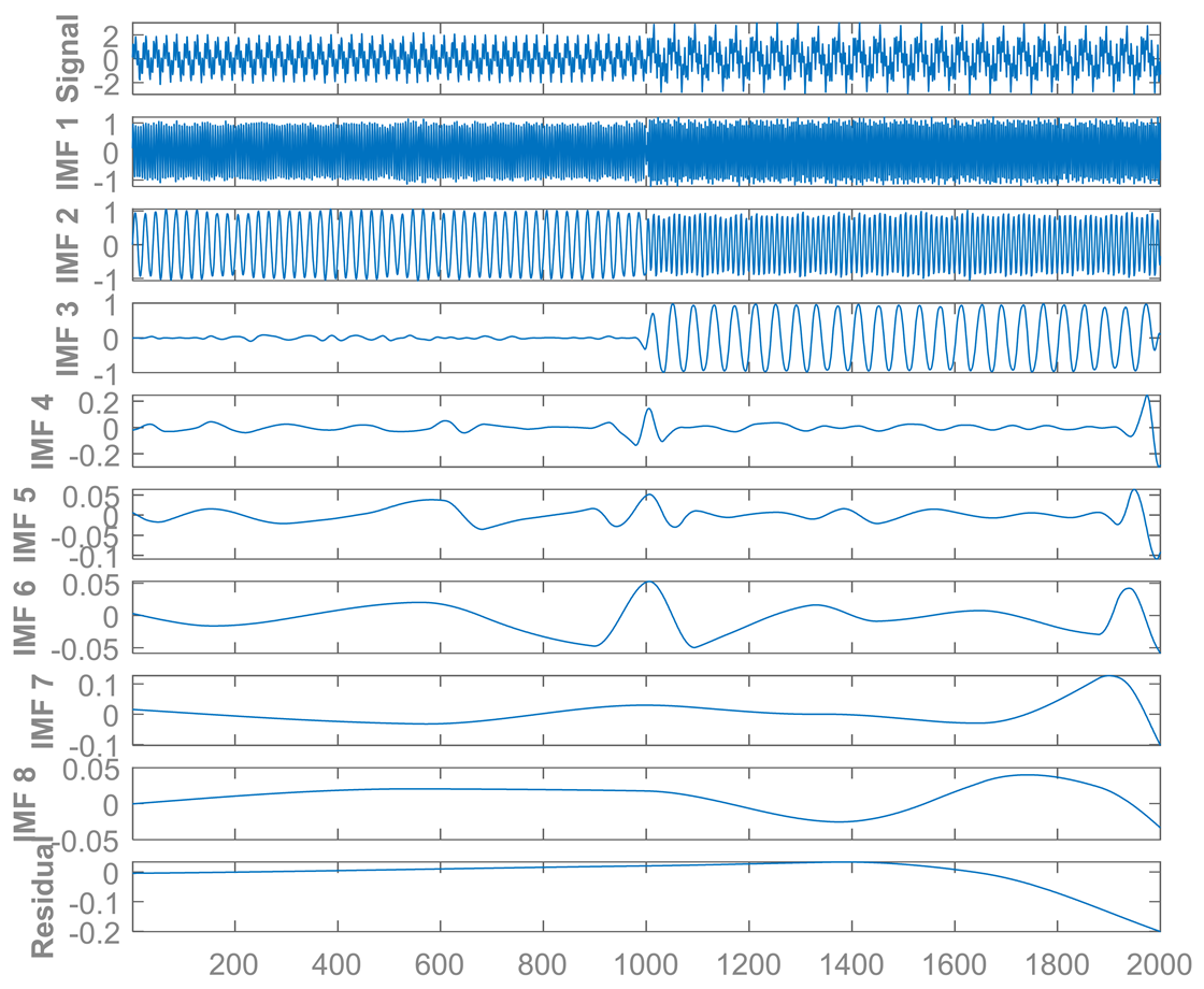
3.1.1. Ensemble Empirical Mode Decomposition

The EMD method [28] is a widely applied non-linear signal adaptive decomposition method. The EMD algorithm has demonstrated a great potential in decomposing a non-stationary and non-linear time series data into IMFs and a residual through an iterative process with individual intrinsic time scale properties [17]. Ensemble EMD (EEMD) is an improved version of the EMD methods, developed by Torres et al. [29], which was aimed at overcoming the problem of intrinsic drawbacks of mode mixing that is associated with the conventional EMD algorithm [17].
EEMD is a noise-aided time series data analysis method. In EEMD method of time series data analysis, white noise is added to enable the separation of contrasting time series scales, which in turn, leads to the improved decomposition efficiency of the EMD method. The introduced white-noise is comprised of components of disparate scale which would systematically fill the entire time-frequency space. The disparate scale components of the signal are spontaneously projected onto proper scales of reference initiated by the Gaussian white-noise, as the systematically distributed white-noise is introduced to the signal. Since all the decomposed components of the introduced Gaussian white-noise consist of both the signal and the introduced white noise, all the individual trials usually end up with noisy results. However, the white-noise can be almost completely cancelled out with the aid of ensemble mean of whole trials, because the white-noise in each of the trials are unique in different trials [30]. Consequently, the actual underlying components of the water quality time series data can be represented by the ensemble mean. In other words, EEMD method sums up the components and adopts the average as the true decomposition results. Finally, the result of decomposition solves the mode mixing drawbacks associated with conventional EMD method. It is a useful method for extracting underlying and crucial components from the water quality time series data.
For the DO time series data x t , the EEMD method follows a certain procedure, which can be described as follows.
Stage 1: Initialize an ensemble number M and the amplitude of the introduced Gaussian white-noise.
Stage 2: Perform the m t h trial for introducing disparate white-noise W m t to x t , in order to generate the noise-augmented time series data x m t , where
x m t = x t + W m t
Stage 3: Determine all the local minima and maxima of x m t and use them to generate both lower and upper envelopes, with the help of cubic spline interpolation functions.
Stage 4: Compute the mean m 1 t of both lower and upper envelopes.
Stage 5: Calculate the difference h 1 t that exists between the mean computed in stage 4 and the signal x m t , using,
h 1 t = x m t m 1 t
Stage 6: If the properties of IMF are satisfied by the h 1 t , that is, from the signal x m t , C 1 t = h 1 t becomes the first IMF component. Otherwise, replace x m t with h 1 t and return to Stage 3.
The two properties of IMF are described as follows: (i) the number of the zero crossing and extrema must either equal or differ at most by 1 over the entire data x t , and (ii) at any given point, the mean value h 1 t of the generated envelopes given by both local minimum and local maximum must be zero.
Stage 7: Separate the residue R 1 t from the rest of the dataset using,
R 1 t = x m t C 1 t
Let the residue R 1 t be a new signal and sift out the remaining IMFs by repeating Stage 3 through Stage 7 n times, until the stopping criterion is satisfied. The applied stopping criterion can be either of the following: (i) when the residue R n t is reduced to a monotonic function such that no more IMF can be extracted from it; (ii) when the residue R n t or IMF component C 1 t becomes smaller than the predetermined value. Then, after the EEMD decomposition process, the original signal x m t can be mathematically expressed as the sum total of each of the IMFs C 1 t components and the residue R 1 t . Hence,
x m t = i = 1 n C i t + R 1 t
where n and C i t denote the total number of the IMFs C 1 t components and the i t h IMF, respectively; and R 1 t represents the final residue.
Stage 8: By adding a different noise in each trial, repeatedly execute Stage 2 to Stage 7 until m = M if m < M , through a consecutive increment of the value of m by using m = m + 1 .
Stage 9: Determine the i t h ensemble mean C i ¯ of the M trials for individual IMF, by way of expression,
C i ¯ = 1 M m = 1 M C i , m                     i = 1 ,   2 ,   3 ,   ,   n  
and the ensemble residue R ¯ n can be expressed as
R ¯ n = 1 M m = 1 M R n , m .
Therefore, the original DO time series data are efficiently decomposed through EEMD method into n ensemble IMFs and a single ensemble residue. In each frequency band, the contained IMF components are individually different, and can change with the variation of the DO dataset x t . Additionally, the ensemble residue denotes the general trend of the DO dataset x t .

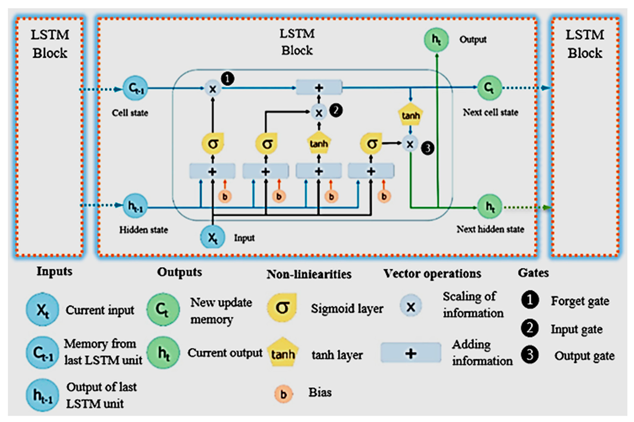
3.1.2. LSTM Neural Network

As depicted by Figure 1, a set of repeating block-chain facilitates effective learning of the time series information by the LSTM NN. The horizontal line (from C t 1 to C t ) which runs from one block to another above the graph is called the cell state. Cell state runs across the blocks with slight linear interactions to ensure that constant state information is maintained [31]. Additionally, LSTM NN uses three different gates (see ❶, ❷, and ❸ in Figure 1). The gates use sigmoid and tanh layer, with a pointwise multiplication to allow for selective passing of information [32]. With the aid of the gates which act as a multi-level feature selector, LSTM NN can memorize or forget information. Other artificial NNs have a common challenge of long-term dependency problem.
Contrarily, LSTM NN is designed to overcome this problem by using gates which control the processes of memorizing necessary information and forgetting the unnecessary information. This helps LSTM NN to forecast the output of the next time series data, based on the feature of the previous time series data. The equation below illustrates the calculation processes involved.
(a)
Forget gate equation:
F t = σ W f × h t 1 , X t + b f
where F t is a vector with values from 0 to 1, with σ , W f , and b f representing the logistic sigmoid function, weight matrices and bias of the forget gate, respectively. From (3), the sigmoid layer determines if the new information is necessary to be used for update or unnecessary and ignored. Then, tanh function adds weight to each value that passed and decides their level of importance ranging from −1 to 1. Similar operations are repeated in input and output gates shown in (8) through (11).
(b)
Input gate equations:
I t = σ W i × h t 1 , X t + b i
I ^ t = tanh W i × h t 1 , X t + b i
(c)
Output gate equations:
O t = σ W o × h t 1 , X t + b o
h t = O t × tanh C t
(d)
Cell state equation:
C t = F t × C t 1 + I t × I ^ t
where W i and W o denote the weight matrixes, b i and b o represent the network’s bias vectors, of the input and output gates. Tanh represents the hyperbolic tangent function.

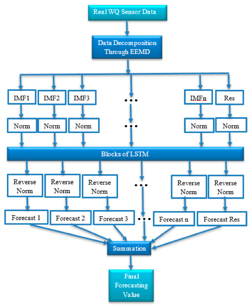
3.1.3. Novel Hybrid EEMD-Based LSTM model

The proposed novel hybrid EEMD-based LSTM forecasting model is depicted in Figure 2. With the proposed new model, the real DO concentration data set is first decomposed by EEMD into several components to improve the forecast accuracy. The detailed procedures illustrated in Figure 2 show the three crucial steps that lead to the development of the new hybrid EEMD-based LSTM forecasting model. In the first step, DO time series data x t are decomposed into several IMFs and a residual item R N t by EEMD algorithm. The data set decomposition is performed through an iterative sifting process, which is expressed as
x t = i = 1 N I M F i t + R N t .
In the second step, each IMF and residual item is normalized and used for forecasting by the LSTM NN. Finally, reverse normalization of individual forecasting results of the LSTM NN is carried out prior to combining all of them together through summation operation to get the final forecasted values, as illustrated in Figure 2. When the final forecasted result is obtained, performance evaluation of the proposed novel hybrid EEMD-based LSTM forecasting model is carried out through the application of three statistical metrics such as mean absolute error (MAE), mean square error (MSE), root mean square error (RMSE), and mean absolute percentage error (MAPE).

4. Experiments and Results

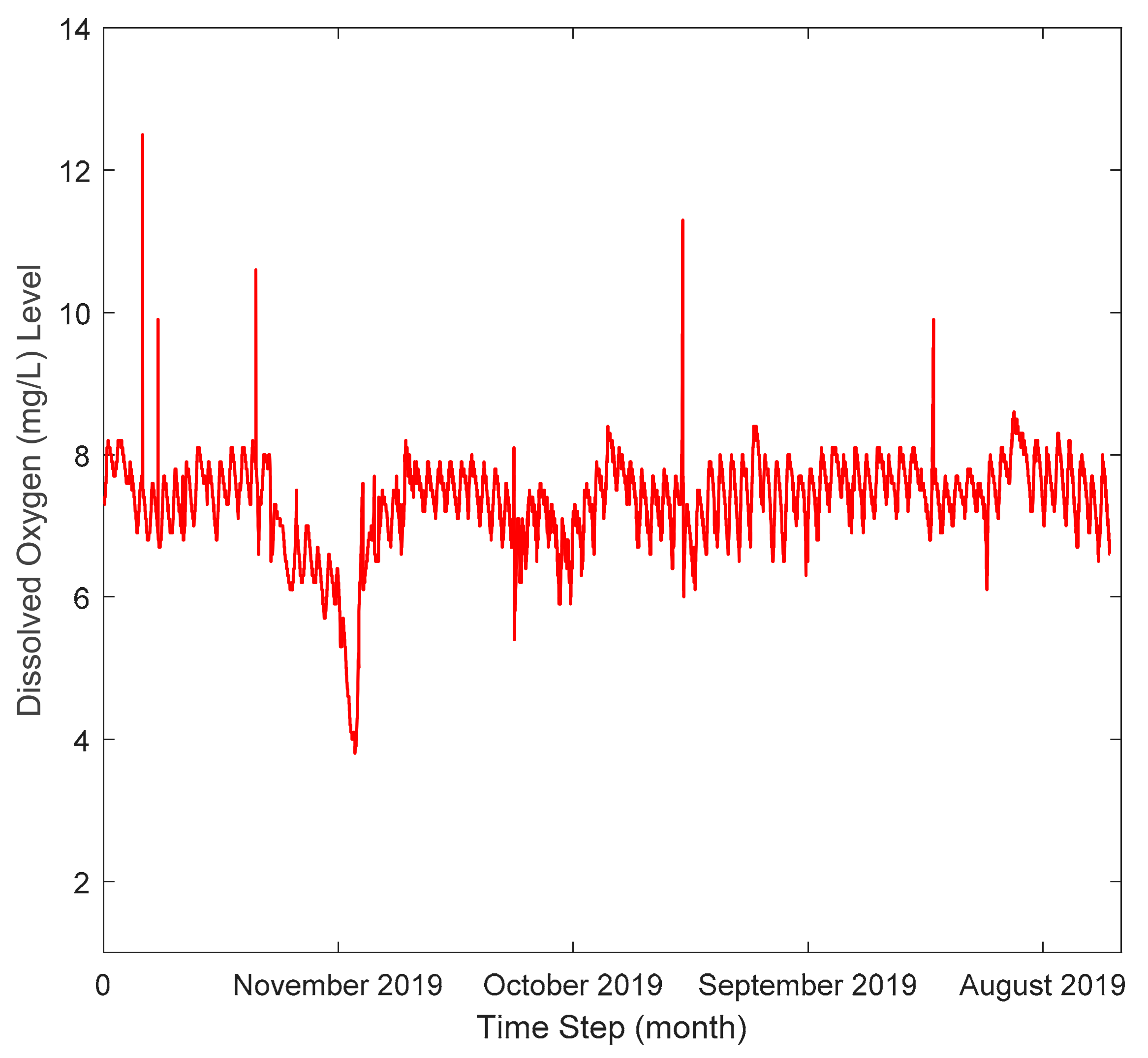
4.1. Water Quality Dataset Acquisition

The data used for the experiments were collected from Laizhou Mingbo mariculture, based at Laizhou City, Shandong Province, China, by a research team at Chinese Agriculture University. A team of researchers from the Chinese Agriculture University visited Laizhou Mingbo farm in Autumn 2019 and collected water quality data. They were responsible for deploying the sensors and their necessary maintenance for the four-month duration of the data collection. The collected raw data consists of seven water quality parameters: DO, pH, water temperature, salinity, Ammonia, and Nitrogen. This choice of parameters is governed by the availability of suitable sensors and the monitoring needs of the mariculture farm. In the presented study, we have investigated forecasting techniques using DO datasets. The reasons for our choice are already indicated in Section 1 and Section 2 above.

4.2. Data Normalization

After pre-processing the sensor data, 12,852 groups of chronological data are used in constructing the improved EMD-based hybrid LSTM forecasting model. The collected water quality data are divided into two parts: the first 75% of the dataset is used for training the developed hybrid model and the last 25% of the dataset is used for model testing in order to analyze the forecasting performance of the proposed novel hybrid EEMD-based LSTM model. The collected raw data are shown in Figure 3. The structural representation of the data set can be expressed as follows:
X = X 𝕥 , 𝕗 N × M = x 11 x 12 x 1 m x 21 x 22 x 2 m x n 1 x n 2 x n m
where X represents the data matrix at a given time step within the time series, x i j represents the j t h feature of i t h week, N and M denote the length and number of features of the time series data, respectively. Finally, the normalization of the data set was done by removing the dimension of each feature using normalization equation, x ˜ i j :
x ˜ i j = x i j mean x · j std x · j
where x ˜ i j denotes the normalized data set, mean x · j represents the mathematical expectation of x · j , and std x · j represents the standard variance of x · j .

4.3. Problem Formulation

Assuming T = 𝕥 1 , 𝕥 2 , , 𝕥 n is the set of time and F = 𝕗 1 , 𝕗 2 , , 𝕗 m is the set of features of the time series data. Then, at time 𝕥 , the value of a feature can be given as a matrix X = X 𝕥 , 𝕗 N × M (see (14)). In X , at time 𝕥 , let x 𝕥 , 𝕗 m and x 𝕗 m represent the value of the target sequence and the feature sequence of the forecast target that is selected, respectively. Therefore, our goal is to forecast the short-term future trends of the target sequence expressed as = x 𝕥 + k , 𝕗 m k 1 , 2 , 3 , , M .

4.4. Performance Evaluation Metrics

In this section, the adopted performance evaluation metrics such as MAE, MSE, RMSE and MAPE were used to measure the forecasting accuracy of the new model. These error metrics show the difference between the forecasted values and original (real DO concentration) values and the smaller the differences; better is the performance of the proposed novel hybrid EEMD-based LSTM forecasting model. The error metrics formulas are given as:
MAE = 1 N i = 1 N V i F i  
MSE = 1 N i = 1 N V i F i 2    
RMSE = 1 N i = 1 N V i F i 2
MAPE = 1 N i = 1 N V i F i V i  
where N denotes the number of data points, V i and F i represent the real and forecasted values, respectively.

5. Discussions

Our study used an hourly centered moving average value for the DO concentration time series data. In this study, EEMD, which is a powerful technique for signal decomposition, was used for decomposing the non-linear and non-stationary signal. Decomposing the DO concentration time series sensor data is an integral part of the proposed hybrid EEMD-based LSTM forecasting model, for forecasting the short-term values of the DO concentration. The adopted EEMD technique decomposed the original DO concentration sensor time series data into eight (8) relatively stable IMFs (IMF 1 to IMF 8) and one residual item (see Figure 4). The EEMD amplitude of Gaussian white noise was set to 0.2. Finally, all the extracted sub-band signals by the adopted EEMD technique were utilized in the decomposition step of the proposed hybrid EEMD-based LSTM forecasting model. The EEMD trend was extracted through the summation of low-frequency IMFs. Figure 5 depicts the non-stationary continuous signal of the real DO concentration composed of sinusoidal waves with a distinct change in frequency.
In Figure 3 is shown the distribution of the collected DO concentration raw dataset; it can be observed that at a certain period, the level of DO concentration dropped to its lowest level, by up to 4.0 mg/L and 3.9 mg/L. The proposed hybrid model was applied in this area and the result is presented in Figure 6. Figure 6 shows the area with DO concentration downward decrease to a meagre 4.0 mg/L up to 3.9 mg/L before picking up again by increasing towards DO concentration of up to 5.25 mg/L. The graphs in Figure 7 and Figure 8 reveal that the new hybrid model provided good results and successfully forecasted DO concentration with a high-level of accuracy for both Short-term forecast and Long-term forecast. It is also noteworthy to mention that Figure 8 illustrates fluctuations in the range of 7.0 mg/L to 8.5 mg/L, which are not critical for aquaculture, since aquatic life can only suffer harm, with a possibility of death, when such DO concentration decreases. Figure 9 shows error graphics of the proposed hybrid EEMD-based LSTM forecasting model performance: short- and long-term forecast.
In Table 1, the error statistics for both short-term and long-term DO content forecasting performance of our proposed hybrid model are shown. The steep increase in error gap between the short-term and long-term DO content forecasting performance of our proposed hybrid model indicates that the nearer the forecast future the higher the forecast accuracy, and vice versa. Figure 9 shows the forecasting error statistics, using bar charts for both short-term and song-term DO concentration to further emphasize the increase in prediction error as the forecasting period increases.
In Table 2, the performance of the proposed hybrid EEMD-based LSTM NN is compared with another related hybrid water quality prediction model, based on sparse auto-encoder (SAE) and LSTM NN, SAE-BPNN, single LSTM and BPNN developed by Li et al. [27]. The tabulated error statistics indicate that our proposed hybrid model outperforms the other models as listed in Table 2, in terms of the error margin of the forecasted data. This performance gain over the other related prediction models is because our proposed hybrid model applied the EEMD method to effectively decompose the original signal into its constituent several intrinsic sub-sequences. Consequently, the proposed hybrid multi-scale forecasting model can get more features through the decomposition process for the forecasted signals, which further results in improved forecasting accuracy. Amongst the models proposed in [27], the hybrid SAE-LSTM model demonstrated the least error in terms of prediction accuracy. However, the tabulated error statistics in Table 2 indicate that our Hybrid EEMD-based LSTM outperforms the SAE-LSTM model, due to the potentials of the applied EEMD method.

6. Conclusions

This paper proposes a hybrid prediction model to solve the challenge of poor DO concentration forecasting accuracy [17,26,27] in aquaculture management. The hybrid model was designed by combining the EEMD technique with LSTM NN. The applied EEMD method allowed for the decomposition of the original sensor data into multiple IMFs. Furthermore, this method is used to carefully select IMFs that are strongly correlated with the original sensor data through a feature selection process, and integrate both into inputs for the neural network. The actual experimental WQ data from a fish farm show that the hybrid model provides good results and outperforms related models with high accuracy, as indicated by error metrics shown in Table 2. For future work, a hybrid EEMD-based multi-variate prediction model can be explored to propose a more comprehensive water quality forecasting and analysis. Additionally, more WQ measuring sites will also be considered to expand this model.

Author Contributions

Conceptualization, E.E. and T.A.; methodology, E.E.; software, E.E.; validation, E.E. and T.A.; formal analysis, E.E.; investigation, E.E.; resources, E.E. and T.A.; data curation, E.E.; writing—original draft preparation, E.E.; writing—review and editing, T.A.; visualization, E.E.; supervision, T.A.; project administration, T.A.; funding acquisition, T.A. All authors have read and agreed to the published version of the manuscript.

Funding

This research was funded by Innovate UK/BBSRC (ref: 86204028, BB/S020896/1).

Acknowledgments

The authors wish to thank their project partners, the researchers at Chinese Agricultural University, for providing the raw data used in this study. The authors also wish to thank the reviewers for their comments and suggestions, which have greatly helped in improving the quality of the paper.

Conflicts of Interest

The authors declare no conflict of interest. The funders had no role in the design of the study; in the collection, analyses, or interpretation of data; in the writing of the manuscript, or in the decision to publish the results.

References

  1. Memon, A.R.; Kulsoom-Memon, S.; Memon, A.A.; Din-Memon, T. IoT Based Water Quality Monitoring System for Safe Drinking Water in Pakistan. In Proceedings of the 2020 3rd International Conference on Computing, Mathematics and Engineering Technologies (iCoMET), Sukkur, Pakistan, 29–30 January 2020; pp. 1–7. [Google Scholar]
  2. Parra, L.; Rocher, J.; Escrivá, J.; Lloret, J. Design and Development of Low-cost Smart Turbidity Sensor for Water Quality Monitoring in Fish Farms. Aquac. Eng. 2018, 81, 10–18. [Google Scholar] [CrossRef]
  3. Mohan, S.; Pavan, K.K. Waste load allocation using machine scheduling: Model application. Environ. Process. 2016, 3, 139–151. [Google Scholar] [CrossRef]
  4. Zhang, Y.F.; Thorburn, P.J.; Fitch, P. Multi-Task Temporal Convolutional Network for Predicting Water Quality Sensor Data. In International Conference on Neural Information Processing; Springer: Cham, Switzerland, 2019; pp. 122–130. [Google Scholar]
  5. Zhang, Y.-F.; Fitch, P.; Thorburn, P.J. Predicting the Trend of Dissolved Oxygen Based on the kPCA-RNN Model. Water 2020, 12, 585. [Google Scholar] [CrossRef] [Green Version]
  6. Parra, L.; Lloret, G.; Lloret, J.; Rodilla, M. Physical Sensors for Precision Aquaculture: A Review. IEEE Sens. J. 2018, 18, 3915–3923. [Google Scholar] [CrossRef] [Green Version]
  7. Parra, L.; Sendra, S.; García, L.; Lloret, J. Design and deployment of low-cost sensors for monitoring the water quality and fish behavior in aquaculture tanks during the feeding process. Sensors 2018, 18, 1–23. [Google Scholar] [CrossRef] [Green Version]
  8. Garcia, M.; Sendra, S.; Lloret, G.; Lloret, J. Monitoring and control sensor system for fish feeding in marine fish farms. IET Commun. 2011, 5, 1682–1690. [Google Scholar] [CrossRef]
  9. Parra, L.; Sendra, S.; Lloret, J.; Rodrigues, J.J. Design and deployment of a smart system for data gathering in aquaculture tanks using wireless sensor networks. Int. J. Commun. Syst. 2017, 30, 1–15. [Google Scholar] [CrossRef]
  10. Xiao, Z.; Peng, L.; Chen, Y.; Liu, H.; Wang, J.; Nie, Y. The Dissolved Oxygen Prediction Method Based on Neural Network. Complexity 2017, 2017, 1–6. [Google Scholar] [CrossRef] [Green Version]
  11. Wijayanti, K.N. Aquaculture water quality prediction using smooth SVM. Iptek J. Proc. 2015, 1, 342–345. [Google Scholar]
  12. Guo, P.; Liu, H.; Liu, S.; Xu, L. Numeric Prediction of Dissolved Oxygen Status Through Two-Stage Training for Classification-Driven Regression. In Proceedings of the 2019 International Conference on Machine Learning and Cybernetics (ICMLC), Kobe, Japan, 7–10 July 2019; pp. 1–6. [Google Scholar]
  13. Xue, H.; Wang, L.; Li, D. Design and Development of Dissolved Oxygen Real-Time Prediction and Early Warning System for Brocaded Carp Aquaculture. In International Conference on Computer and Computing Technologies in Agriculture; Springer: Berlin/Heidelberg, Germany, 2012; pp. 35–42. [Google Scholar]
  14. Liu, J.; Yu, C.; Hu, Z.; Zhao, Y.; Bai, Y.; Xie, M.; Luo, J. Accurate Prediction Scheme of Water Quality in Smart Mariculture with Deep Bi-S-SRU Learning Network. IEEE Access 2020, 8, 24784–24798. [Google Scholar] [CrossRef]
  15. Yan, J.; Gao, Y.; Yu, Y.; Xu, H.; Xu, Z. A Prediction Model Based on Deep Belief Network and Least Squares SVR Applied to Cross-Section Water Quality. Water 2020, 12, 1929. [Google Scholar] [CrossRef]
  16. Liu, S.; Tai, H.; Ding, Q.; Li, D.; Xu, L.; Wei, Y. A hybrid approach of support vector regression with genetic algorithm optimization for aquaculture water quality prediction. Math. Comp. Mod. 2013, 58, 458–465. [Google Scholar] [CrossRef]
  17. Li, C.; Li, Z.; Wu, J.; Zhu, L.; Yue, J. A hybrid model for dissolved oxygen prediction in aquaculture based on multi-scale features. Inf. Proc. Agric. 2018, 5, 11–20. [Google Scholar] [CrossRef]
  18. Junsheng, C.; Kang, Z.; Yu, Y.; De-jie, Y.U. Comparison between the methods of local mean decomposition and empirical mode decomposition. J. Vib. Shock 2009, 28, 13–16. [Google Scholar]
  19. Beltrán-Castro, J.; Valencia-Aguirre, J.; Orozco-Alzate, M.; Castellanos-Domínguez, G.; Travieso-González, C.M. Rainfall Forecasting Based on Ensemble Empirical Mode Decomposition and Neural Networks. In International Work-Conference on Artificial Neural Networks; Springer: Berlin/Heidelberg, Germany, 2013; pp. 471–480. [Google Scholar]
  20. Tian, Z. Approach for Short-Term Traffic Flow Prediction Based on Empirical Mode Decomposition and Combination Model Fusion. IEEE Tran. Int. Trans. Syst. 2020. [Google Scholar] [CrossRef]
  21. Chen, X.; Lu, J.; Zhao, J.; Qu, Z.; Yang, Y.; Xian, J. Traffic Flow Prediction at Varied Time Scales via Ensemble Empirical Mode Decomposition and Artificial Neural Network. Sustainability 2020, 12, 3678. [Google Scholar] [CrossRef]
  22. Pholsena, K.; Pan, L.; Zheng, Z. Mode decomposition based deep learning model for multi-section traffic prediction. World Wide Web 2020, 23, 2513–2527. [Google Scholar] [CrossRef] [Green Version]
  23. Zhang, G.; Liu, H.; Zhang, J.; Yan, Y.; Zhang, L.; WU, C. Wind power prediction based on variational mode decomposition multi-frequency combinations. J. Mod. Power Syst. Clean Energy 2019, 7, 281–288. [Google Scholar] [CrossRef] [Green Version]
  24. Liu, K.; Zhang, Y.; Qin, L. A novel combined forecasting model for short-term wind power based on ensemble empirical mode decomposition and optimal virtual prediction. J. Renew. Sustain. Energy 2016, 8, 1–22. [Google Scholar] [CrossRef]
  25. Liu, S.; Xu, L.; Li, D. Multi-scale prediction of water temperature using empirical mode decomposition with back-propagation neural networks. Comp. Elec. Eng. 2016, 49, 1–8. [Google Scholar] [CrossRef]
  26. Liu, S.; Yan, M.; Tai, H.; Xu, L.; Li, D. Prediction of Dissolved Oxygen Content in Aquaculture of Hyriopsis Cumingii Using Elman Neural Network. In International Conference on Computer and Computing Technologies in Agriculture; Springer: Berlin/Heidelberg, Germany, 2011; pp. 508–518. [Google Scholar]
  27. Li, Z.; Peng, F.; Niu, B.; Li, G.; Wu, J.; Miao, Z. Water Quality Prediction Model Combining Sparse Auto-encoder and LSTM Network. IFAC-PapersOnLine 2018, 51, 831–836. [Google Scholar] [CrossRef]
  28. Huang, N.E.; Zheng, S.; Long, S.R.; Wu, M.C.; Shih, H.H.; Zheng, Q.; Yen, N.-C.; Tung, C.C.; Liu, H.H. The empirical mode decomposition and the Hilbert spectrum for nonlinear and non-stationary time series analysis. Proc. R. Soc. Lond. A Math. Phys. Eng. Sci. 1998, 454, 903–995. [Google Scholar] [CrossRef]
  29. Torres, M.E.; Colominas, M.A.; Schlotthauer, G.; Flandrin, P. A Complete Ensemble Empirical Mode Decomposition with Adaptive Noise. In Proceedings of the 2011 IEEE International Conference on Acoustics, Speech and Signal Processing (ICASSP), Prague, Czech Republic, 22–27 May 2011; pp. 4144–4147. [Google Scholar]
  30. Wu, Z.H.; Huang, N.E. Ensemble empirical mode decomposition: A noise assisted data analysis method. Adv. Adapt. Data Anal. 2009, 1, 1–41. [Google Scholar] [CrossRef]
  31. Wang, H.; Raj, B. On the origin of deep learning. arXiv 2017, arXiv:1702.07800. [Google Scholar]
  32. Shao, X.; Kim, C.S. Multi-Step Short-Term Power Consumption Forecasting Using Multi-Channel LSTM with Time Location Considering Customer Behavior. IEEE Access 2020, 8, 125263–125273. [Google Scholar] [CrossRef]
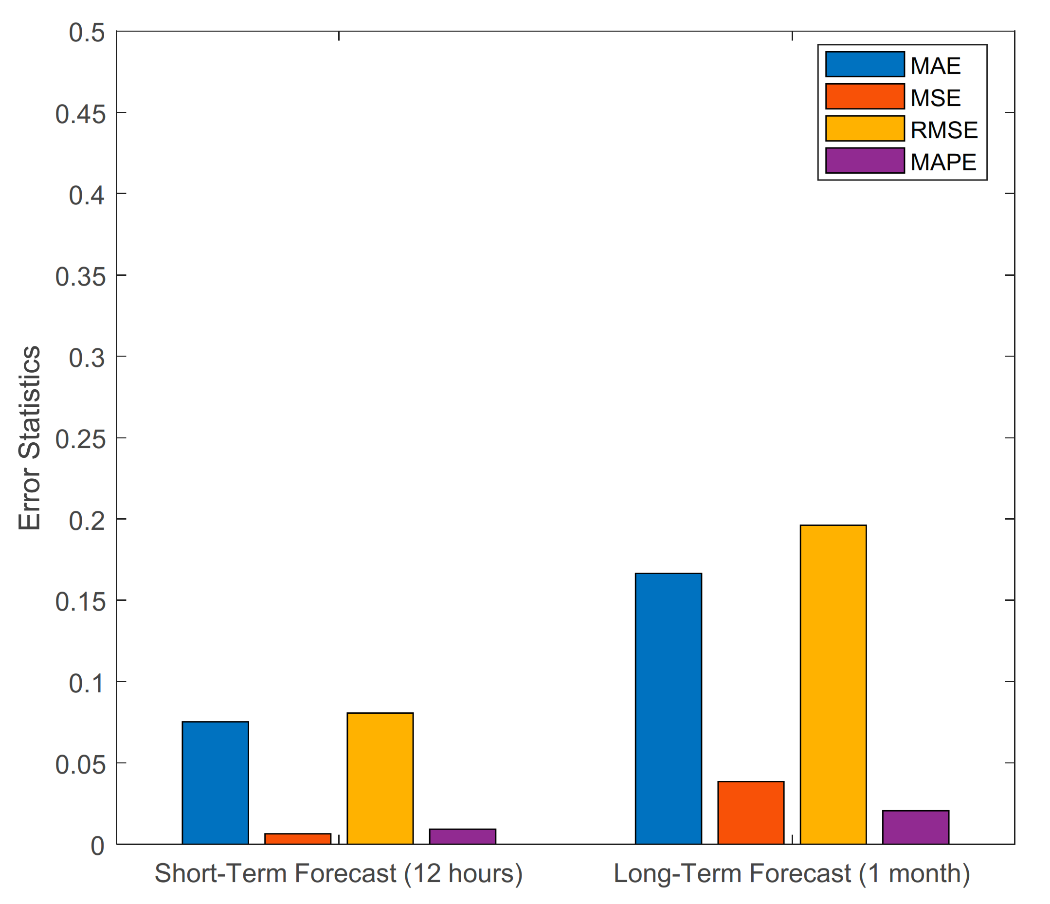
Figure 1. The structure of long short-term memory (LSTM) neural networks (NN) blocks with their corresponding symbols and meanings.
Applsci 10 07079 g001
Figure 2. Hybrid ensemble empirical mode decomposition (EEMD)-based LSTM model architecture.
Applsci 10 07079 g002
Figure 3. Four months’ distribution of the DO concentration raw data.
Applsci 10 07079 g003
Figure 4. Decomposition by EEMD illustrating 8 out of 8 intrinsic mode functions (IMFs).
Applsci 10 07079 g004
Figure 5. Non-stationary continuous signal composed of sinusoidal waves with a distinct change in frequency.
Applsci 10 07079 g005
Figure 6. Short-term (6 h) forecast result measured against actual dissolved oxygen (DO) concentration values.
Applsci 10 07079 g006
Figure 7. Short-term (12 h) forecast result measured against actual DO concentration values.
Applsci 10 07079 g007
Figure 8. Long-term forecast result measured against actual DO concentration values.
Applsci 10 07079 g008
Figure 9. Forecasting error statistics for short-term and long-term DO concentration.
Applsci 10 07079 g009
Table 1. Error Statistics for Short-term and Long-term DO Content Forecasting.
Error Statistics12 Hour Forecast1 Month Forecast
MAE0.07530.1666
MSE0.00650.0385
RMSE0.08070.1962
MAPE0.00930.0206
Table 2. Performance Comparison with Related Forecasting Models *.
Error
Statistics
LSTM
NN
BPNNSAE-LSTM NNSAE-BPNNEEMD-LSTM NN
Run Time(s)23.23.629.69.12.37
MAE0.15900.45300.12600.40600.0753
MSE0.03980.30130.02420.24280.0065
RMSE0.19950.54890.15560.49270.0807
MAPE0.01600.04500.01300.04190.0093
* Back-propagation neural network (BPNN) model, radial basis function neural network (RBFNN) model, long short-term memory (LSTM) model, sparse auto-encoder (SAE) and LSTM (SAE-LSTM) NN model, and SAE-BPNN model [27], and our proposed ensemble EMD based LSTM (EEMD-LSTM) NN model.

