Article

Comparison of Spectral Reflectance-Based Smart Farming Tools and a Conventional Approach to Determine Herbage Mass and Grass Quality on Farm

1
Competitiveness and System Evaluation, Agroscope, Tänikon 1, 8356 Ettenhausen, Switzerland
2
Institute of Agricultural Sciences in the Tropics, University of Hohenheim, Fruwirthstrasse 31, 70599 Stuttgart, Germany
3
Animal Production Systems and Animal Health, Agroscope, Reckenholzstrasse 191, 8046 Zurich, Switzerland
4
Methods Development and Analytics, Agroscope, Rte de la Tioleyre 4, 1725 Posieux, Switzerland
*
Author to whom correspondence should be addressed.
Remote Sens. 2020, 12(19), 3256; https://doi.org/10.3390/rs12193256
Submission received: 11 September 2020 / Revised: 29 September 2020 / Accepted: 2 October 2020 / Published: 7 October 2020
(This article belongs to the Special Issue Remote Sensing of Grassland Ecosystem)

Abstract

:
The analysis of multispectral imagery (MSI) acquired by unmanned aerial vehicles (UAVs) and mobile near-infrared reflectance spectroscopy (NIRS) used on-site has become increasingly promising for timely assessments of grassland to support farm management. However, a major challenge of these methods is their calibration, given the large spatiotemporal variability of grassland. This study evaluated the performance of two smart farming tools in determining fresh herbage mass and grass quality (dry matter, crude protein, and structural carbohydrates): an analysis model for MSI (GrassQ) and a portable on-site NIRS (HarvestLabTM 3000). We compared them to conventional look-up tables used by farmers. Surveys were undertaken on 18 multi-species grasslands located on six farms in Switzerland throughout the vegetation period in 2018. The sampled plots represented two phenological growth stages, corresponding to an age of two weeks and four to six weeks, respectively. We found that neither the performance of the smart farming tools nor the performance of the conventional approach were satisfactory for use on multi-species grasslands. The MSI-model performed poorly, with relative errors of 99.7% and 33.2% of the laboratory analyses for herbage mass and crude protein, respectively. The errors of the MSI-model were indicated to be mainly caused by grassland and environmental characteristics that differ from the relatively narrow Irish calibration dataset. The On-site NIRS showed comparable performance to the conventional Look-up Tables in determining crude protein and structural carbohydrates (error ≤ 22.2%). However, we identified that the On-site NIRS determined undried herbage quality with a systematic and correctable error. After corrections, its performance was better than the conventional approach, indicating a great potential of the On-site NIRS for decision support on grazing and harvest scheduling.

Graphical Abstract

1. Introduction

For many years, indoor housing has been preferred by dairy producers because feeding and caretaking on an individual animal level was simpler and more labor-saving compared to grazing-based systems [1,2]. Currently, due to modern technology that addresses both labor requirements and precision feed supply on pastures, grazing-based dairy production systems are viable again [3,4]. In grazing-based production systems, knowing herbage quantity and quality is key to an efficient use of the grassland resource because it enables defining adequate stocking rates, optimizing grazing and harvest scheduling, and refining herbage feeding and concentrate supplementation [5,6].
In Switzerland, the rate of grass growth varies widely within each growing season and between years [7]. Moreover, the range of pedoclimatic conditions, topographies, and expositions under which grasslands are used for forage production is vast. Correspondingly, the spatial variability of grassland yield is very large [8]. As it is time-consuming to accurately measure herbage growth or grassland yields, farmers usually settle for a rough estimation. Many farmers estimate standing herbage mass from visual observation or increasingly by means of a rising plate meter [9]. To accurately estimate herbage mass, the rising plate meter requires labor-intensive re-calibration for assessing the specific plots [5], which leads to a trade-off between labor costs and accuracy. Rising plate meters are, moreover, only suited for measuring low grasslands in the early growth stages [9].
The quality of herbage as livestock feed is also widely variable. The quality highly depends on the growth stage, and thus, on the timing of cutting and grazing [10]. Furthermore, the quality is subjected to large seasonal variability [6] and is influenced by the weather conditions that prevail during the weeks preceding harvesting [11]. Moreover, the plant species composition is also an important influential factor [12]. On commercial farms, herbage quality is rarely determined, as no convenient method is available. Obtaining accurate information about herbage quality by means of laboratory analyses requires proper, representative herbage sampling, which is a difficult task at farm scale. Moreover, the high cost and latency until delivery of the results often render laboratory analyses unsuitable for farmers because decisions, such as time of meadow harvest, are made short term, depending on the weather forecast.
A conventional alternative to laboratory analyses is to visually assess the grassland in the field and determine herbage quality based on look-up tables, such as the look-up tables by Daccord et al. [10] for Swiss grasslands. The reference values by Daccord et al. [10] consider important influencing factors. Pure stands and seven types of multi-species grasslands are distinguished according to their botanical composition, and five growth stages are differentiated. Quality is assumed to be constant over the year, apart from differentiating the first growth and the subsequent regrowth [10]. An advantage of such reference values is that they enable farmers to obtain a real-time rough estimate of herbage quality. A disadvantage is that this method requires the farmer to determine the growth stage and grassland botanical composition, which is a challenging task for multi-species grasslands [13]. An obvious disadvantage is furthermore that look-up tables cannot capture the full natural variation as only a limited number of sward characteristics are included.
In overcoming the limitations of the conventional methods, such as the use of rising plate-meters and look-up tables, spectral reflectance-based smart farming tools might play a major role. With spectral reflectance analysis, the biomass and quality of herbaceous matter is determined based on the spectral signature of the material [14,15]. One commonly employed method is near-infrared reflectance spectroscopy (NIRS), which was proposed for quality measurements of animal feed in the 1970s [16]. Since then, several calibration studies were undertaken to determine the characteristics and nutrient concentrations in herbage, haylage, and grass silage [17,18,19,20]. NIRS instruments can accurately measure these feed quality features when used under laboratory conditions on dried and milled samples, given an adequate calibration dataset [21]. In recent years, NIR spectrometers were integrated into smart-farming tools that directly analyze fresh herbage without prior drying and milling of a sample. These tools are available as portable laboratories to work on-site or are mounted onto harvest machinery to measure in real time (HarvestLabTM 3000, Deere & Company, Moline, IL, USA; AgriNIR, Dinamica Generale, Poggio Rusco, Italy; Moisture TrackerTM, Digi-Star, Fort Atkinson, WI, USA; Polytec NIRS, Haldrup, Ilshofen, Germany; NIR4 Farm, Aunir, UK). With portable NIRS instruments, it is a major challenge to achieve the same level of accuracy as laboratory NIRS [19,22,23]. The difficulty in analyzing field-fresh matter without prior drying and milling is that the heterogeneity of the plant material, its particle size, and the moisture content affect the light reflectance [19,21]. The spectral signature of water can mask signals, which are important for the quantification of dry matter quality parameters, such as crude protein concentration [15,24].
Methods that are based on remote sensing are recent alternatives to NIRS for estimating herbage mass and quality of grassland [25,26,27,28]. Most of these methods use multispectral imagery collected from satellites or unmanned aerial vehicles [26,29]. Analyzing grasslands with remote sensing is particularly promising because it is non-destructive, can potentially capture large areas, and resolves spatial variability typically better than methods based on point sampling. Unfortunately, multispectral imagery only captures the surface of the vegetation with limited information on the subjacent material. Estimating grassland properties from multispectral imagery might, therefore, be error-prone, particularly for high-biomass swards [26].
Both NIRS and multispectral imaging methods indirectly determine herbage quantity and quality and require calibration against a reference method, such as oven-drying or wet chemical analysis. However, the calibrations need to cover a large heterogeneity in grassland types and a large variability of grassland conditions during the vegetation period to establish high accuracy. If calibrations are applied to grassland types and conditions not included in the training data set, it is not always applicable to generalize the results.
The aim of this study was to evaluate two spectral-reflectance-based smart farming tools for determining herbage mass and quality of multi-species grasslands—a portable NIRS and a model to analyze multispectral imagery—and to compare them to the conventional approach of estimating herbage quality with look-up tables. Using grasslands of contrasting botanical composition and multiple harvests during the whole vegetation period, the accuracy of the tools by comparison with laboratory measurements was examined. Further, the relationships between the apparent errors and the grassland characteristics were investigated to identify potential causes. The smart farming tools were put into context with the conventional approaches for assessing grassland quality.

2. Materials and Methods
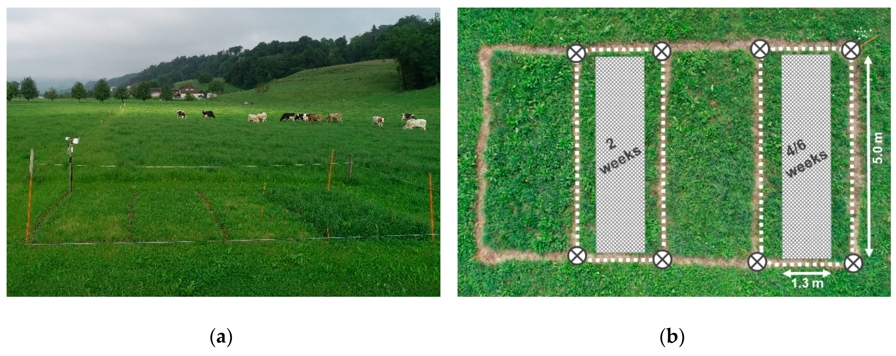
2.1. Experiments

2.1.1. Grassland Study Sites

Herbage mass and quality parameters were measured on 18 grassland plots, which were distributed over six commercial farms in Switzerland. The studied grasslands are described in Figure 1 and Table S1. Prior to this study, the grasslands were used for intensive silage or hay production, with four to six defoliations per year and regular fertilization. With the exception of two grasslands, they were permanent grasslands that were sown less than five years ago (MT3 and SI2, Table S1). The plant communities comprised between 13 and 27 species (Table S1), with relative abundances of 6–75% ryegrasses, 13–59% other grasses, 1–15% clover species, and 2–48% herbs (Figure 1).

2.1.2. Experimental Design

On each commercial farm, three plots were distributed spatially over the intensively managed grassland area of the farms. On each plot, measurements were performed on two different subplots with dimensions of 2.2 m × 5.0 m (Figure 2). On the two subplots, we simulated two different defoliation regimes, which correspond to intensive grazing conditions and silage production. The first subplot, simulating grazing conditions, was defoliated every two to three weeks, at an early phenological stage. Sampling was conducted every second defoliation and always at an age of two weeks. The second subplot, simulating silage production, was defoliated every four to six weeks. The defoliation dates corresponded with the sampling dates. These dates were scheduled to meet the early heading phenological stage; thus, a more mature stage compared to the grazing simulation. The dates of defoliation, therefore, differed among farms according to the climatic conditions of the sites. Therefore, the two defoliation regimes are subsequently referred to as “two weeks of growth” for simulated grazing conditions and “four to six weeks of growth” for the silage production system.
Both defoliation regimes were planned to be observed on five dates each within the vegetation period. Therefore, we aimed for a total number of 180 observations. However, due to a severe drought during summer and autumn, herbage growth was reduced, and three sampling dates had to be omitted at farms BL and BB. Hence, we obtained a total of 162 herbage samples.
All sampling dates were subsequently assigned to one of the four categories to study the effect of the growth period on herbage mass and quality: April to May (representing the first regrowth after winter dormancy), May to June (representing the second cut), June to August (representing the third and fourth cuts), and August to October (representing the fourth and fifth cuts).

2.1.3. Herbage Sampling

To sample the subplots with the four- to six-week old herbage, a double-knife motor mower was used to cut the herbage at 5 cm above-ground, and fresh herbage mass (HM) of 6.5 m2 (central 1.3 m of the 2.2 m wide subplots × 5 m) was determined (Figure 2). A representative sample was taken by stabbing a metal cylinder with a diameter of 5 cm into the pile of cut herbage.
For the first sampling of the two-week-grown herbage, the same method was applied as described above. For the subsequent sampling dates, a randomly selected 1 m2 area of the subplot was sampled at 5 cm above-ground with an electronic hand shear (2 m2 were sampled in case of very low HM). Fresh HM was determined, and the whole sample was used for further analyses.

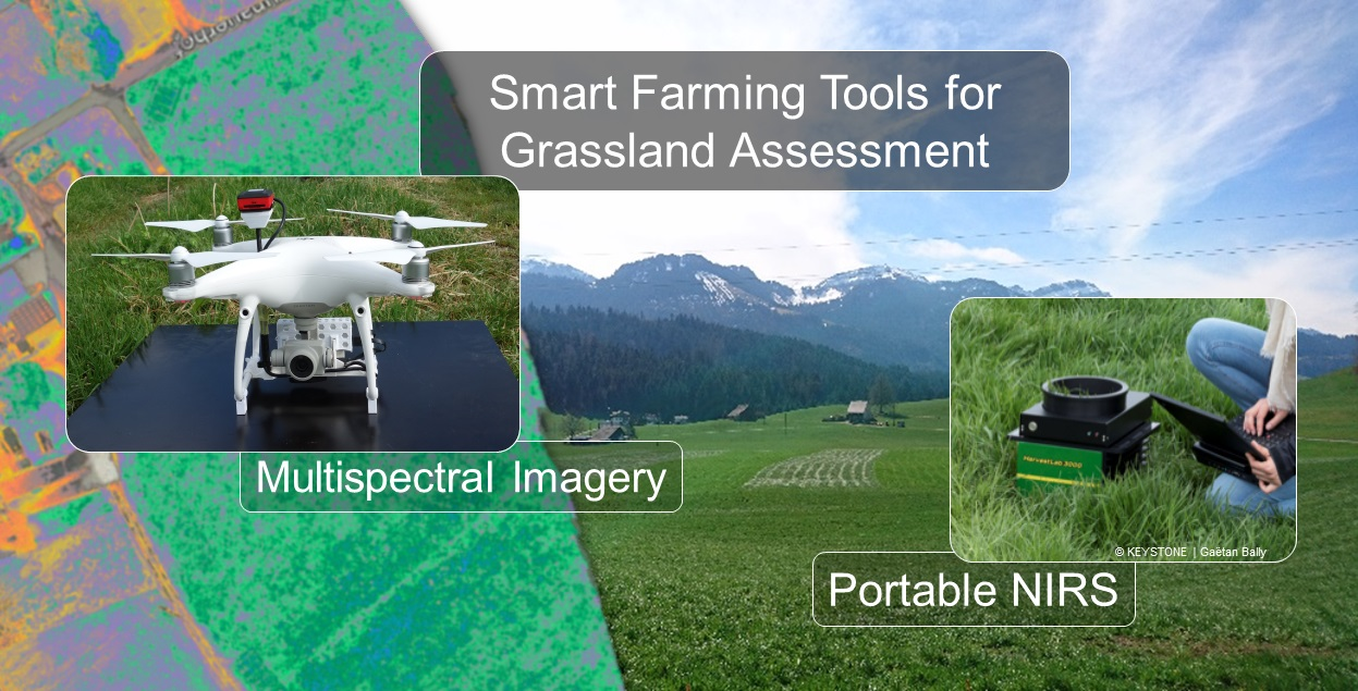
2.2. Smart Farming Tools

2.2.1. Multispectral Imagery Model

The multispectral imagery model (MSI-model) was provided on the open access platform GrassQ (www.grassq.com). According to Murphy et al. [30], GrassQ is a holistic precision herbage measurement and analysis system that analyzes the reflectance data captured by unmanned aerial vehicles (UAVs) or satellites above grasslands on a farm parcel level in nearly real time. For this study, the platform was employed between 2 January 2019 and 2 July 2019. The MSI-model development was based on data of UAV surveys above field plots and grazed paddocks containing mainly perennial ryegrass and clover mixtures at Moorepark (Teagasc Research Centre, Fermoy, Cork, Ireland) on six days in 2017 and 2018 [31]. The calibration range for HM is 304.6 to 2435.7 kg dry matter (DM) ha−1 and for crude protein (CP) 126.3 to 247.3 g kg−1 DM. The models were derived by stepwise multiple linear regression analysis and are referred to as BM-5 and CPM-5 in Askari et al. [31].
In this study, we chose comparable flight characteristics and used the same sensor utilized by Askari et al. [31]. MSI was acquired two hours before cutting the subplots at maximum. We used a Parrot Sequoia multispectral camera (Parrot SA, Paris, France) that was mounted on a UAV (quadcopter, DJI Phantom 4 Pro+, DJI, Shenzhen, China). Both a sequoia sunshine sensor and a calibrated reference panel (Airinov, Paris, France) were employed for radiometric correction. Images were taken during autonomous flights over the experimental plots. The flight missions were planned in the field using the smart device App Pix4D Capture (Version 4.5.0, build 2348, Pix4D, Lausanne, Switzerland). The flight and imagery settings were as follows: flight height of 50 m, flight speed of 5 m s−1, double grid mission, image capturing every 1.9 s, and image overlap of ≥ 80%. Spectral information was recorded for the green, red, red-edge, and near-infrared (NIR) bands that were centered at 550 nm, 660 nm, 735 nm, and 790 nm, respectively. The bandwidth was 40 nm, except for the red-edge, which had a bandwidth of 10 nm. The average ground sampling distance was 5 cm. Due to dense fog and rainy weather, images could not be taken at three sampling dates. Additional data points were not considered for analysis because of the low image quality, resulting in 15 excluded and 147 remaining MSI data points.
The raw MSI was processed with the photogrammetry software Pix4D Mapper with default settings and radiometric correction based on reference panel images (Version 4.3.31, Pix4D, Lausanne, Switzerland). The resulting reflectance maps were georeferenced using at least three of the eight ground control points at each experimental plot (Figure 2), which were measured using a real-time kinematic global navigation satellite system (RTK GNSS), Trimble R8, Sunnyvale, CA, USA). After georeferencing, the absolute horizontal accuracy of the reflectance maps was less than 6 cm. The reflectance maps of the four bands (green, red, red-edge, and NIR) were uploaded to the GrassQ platform (www.grassq.com), and the model that uses UAV-acquired MSI reflectance maps was executed (hereafter referred to as MSI-model). The CP results (as g kg−1 DM) and HM results (as kg DM ha−1) were given as mean values per subplot by the MSI-model, which we extracted by uploading the spatial boundary coordinates.

2.2.2. On-Site NIRS

The portable NIRS instrument (HarvestLabTM 3000, Deere & Company, Moline, IL, USA), hereafter referred to as On-site NIRS, can be operated as a mobile laboratory either in farm offices or car boots or mounted onto harvest machinery to analyze feed quality in the field and in nearly real time. The instrument consisted of a sensor body with the diode array spectrometer and a sampling unit with a rotating sampling dish above a halogen light source. The system operated with internal black and white references and measured wavelengths between 950 nm and 1530 nm at a spectral resolution of 3–2 nm. Selectable calibration models were available for different fodder crops. We evaluated the system for measuring fresh herbage quality using the calibration version 2017/21/03. The instrument was delivered and put into operation by a service technician approximately six weeks before the start of the study. The calibration models, therefore, were based on the reference methods described in VDLUFA [32] and were analog to the wet-chemical analyses in our study. During field sampling, fresh herbage was analyzed using the On-site NIRS in the open boot of a car. The measurement was performed immediately after herbage sampling as described above. Due to the missing manufacturer’s specifications, a particle length of approximately 5 cm was chosen and obtained by stabbing with a metal cylinder. A representative part of the sampled herbage was filled in the instruments’ sampling dish. Care was taken to assure that the sampling dish was clean and dry. The measurement was repeated three times with mixing of the subsample in between. Mean values of DM concentration and mean values of CP, crude fiber (CF), acid detergent fiber (ADF), and neutral detergent fiber (NDF) as concentrations of DM were recorded.

2.3. Conventional Method

Additional to the two smart farming tools, the herbage quality parameters (DM, CP, CF, ADF, and NDF) were determined by using look-up tables for herbage quality of multi-species grasslands by Daccord et al. [10], hereafter referred to as Look-up Tables. For this reason, the number and relative abundance of plant species were visually surveyed in April/May and a second time in July/August. The average of both surveys was used to determine the herbage categories according to Table 13.1 in Daccord et al. [10], where the seven categories distinguish between grass-rich, legume-rich, herb-rich, and grass-legume-herb-balanced multi-species grasslands. At the first sampling date in spring, the phenological stage was determined by direct visual observation. The following determinations of the phenological stage were performed using Table 13.2 in Daccord et al. [10], considering the time period since last defoliation.

2.4. Laboratory Analysis

The herbage samples were oven-dried at 60 °C for 48 h and weighed to determine DM as a percentage of fresh matter (FM). The HM in kg DM ha−1 was calculated for each subplot based on the area that was cut and weighed during field sampling. A dried subsample was milled to pass a 1 mm sieve (Brabender, Duisburg, Germany). Between 100 g and 200 g of a milled sample were analyzed using a laboratory NIRS measuring wavelengths in the range of 1000–2500 nm at a spectral resolution of 8 cm−1 (Fourier-transform NIR; NIRFlex N-500 system; Büchi, Flawil, Switzerland). The calibration model for CP, CF, NDF, and ADF is shown in Table S2. The laboratory NIRS was used as a reference method to evaluate the performance of the herbage quality determination by the On-site NIRS and the MSI-model (Table 1).
To validate the laboratory NIRS, a milled subsample of one third of the herbage samples was subjected to wet-chemical analyses. The selected samples covered all farms and sampling dates and represented the observed variation in herbage composition well (Table S1). The DM determination was based on ISO 6496:1999 with the following modifications: 1–2 g of sample were heated in a prepASH system (Precisa instruments AG, Dietikon, Switzerland) at 105 °C for 3 h to reach constant weight. The CP was determined using the Dumas method (ISO 16634-1:2008), and CF was analyzed based on ISO 6865:2000 with the modifications that 0.5 g of the sample were treated in a FIBRETHERM FT12 system (C. Gerhardt GmbH & Co. KG, Königswinter, Germany). The concentration of ADF and NDF were measured using the FT12 system following the methods AOAC 973.18 and ISO 16472:2006, respectively, and expressed based on the organic matter content (ash-free dry weight). Prior to the NDF determination, the sample was treated with a heat stable amylase. Table 2 gives an overview of the wet chemical methods that were used to validate the laboratory NIRS herbage parameters.

2.5. Statistical Analysis

Agreement of the On-site NIRS and the MSI-model with the reference methods was assessed with Lin’s concordance correlation coefficient (CCC) [33], which ranges from −1 to +1. CCC considers both the linear correlation between the methods and the distance between the line of best fit to the line of identity (1:1 line). Agreement was considered negligible (x ≤ 0.30), slight (0.30 < x ≤ 0.50), minor (0.50 < x ≤ 0.70), moderate (0.70 < x ≤ 0.90), strong (0.90 < x ≤ 0.95), and very strong (x > 0.95).
Linear relationships were determined with Pearson’s correlation coefficient (rp). We used ordinary least squares multivariate linear regression to explain the errors of the MSI-model (reference − MSI-model). Significance of the explanatory variables was determined with the F-test using Type III sums of squares (significance when added last). The relative importance of the explanatory variables, i.e., individual contributions to the explained variance of the linear model (R2), was calculated with Lindemann, Merenda, and Gold (LMG) metrics according to Lindemann et al. [34].
To determine the systematic error components for the On-site NIRS versus the reference method, we applied Passing–Bablok linear regression, which takes into account the imprecision of both X and Y [35]. The 95% confidence band and the two-sided 95% confidence intervals of slope and intercept were determined using bootstrapping. A significant systematic error between the comparison method and the reference method is indicated when the confidence interval of the intercept does not contain 0 (= constant error) and/or the confidence interval of the slope does not contain 1 (= proportional error).
To investigate the potential for improvement of the On-site NIRS method, we corrected the systematic errors using the Passing–Bablok regression results as follows:
Y corrected = Y I + S 1 X ref ,
where Ycorrected and Y are the corrected values and the original On-site NIRS values, respectively; I is the intercept; S is the slope; and Xref is the value of the reference method. In addition to the correction using the regression results from fitting the complete dataset, we corrected in a leave-one-farm-out fashion, where the regression model fitted to the data from five farms was used to correct the data of the left-out sixth farm (all regression parameter estimates in Table S3). The software R was employed for all statistical analyses (Version 3.5.3, R Foundation). The R package epiR [36] was employed for CCC analysis. Passing–Bablok regression was performed using the mcr package [37]. Multivariate linear regression models were fitted with the base R function lm. The significance of individual explanatory variables was calculated using the base R function drop1, and the R package relaimpo [38] was used to calculate the LMG relative importance metrics.

3. Results

3.1. Validation of the Laboratory NIRS as a Reference Method

The laboratory NIRS results showed a strong concordance with the wet-chemical analysis results for the herbage quality parameters CP, CF, and NDF (Figure S1). The values of rp for CP and CF were 0.943 and 0.930, respectively, and the values of CCC were 0.94 and 0.93, respectively. For ADF and NDF, rp and CCC were slightly lower than for CP and CF (ADF: rp 0.896, CCC 0.89; NDF: rp 0.906, CCC 0.91), which shows a moderate concordance for ADF. Nevertheless, the mean absolute percentage error of the laboratory NIRS remained below 5.2% for all parameters (5.15% for CP, 4.06% for CF, 4.90% for ADF, and 3.76% for NDF), which justifies the use of the laboratory NIRS as a reference method for evaluation of the smart farming tools.

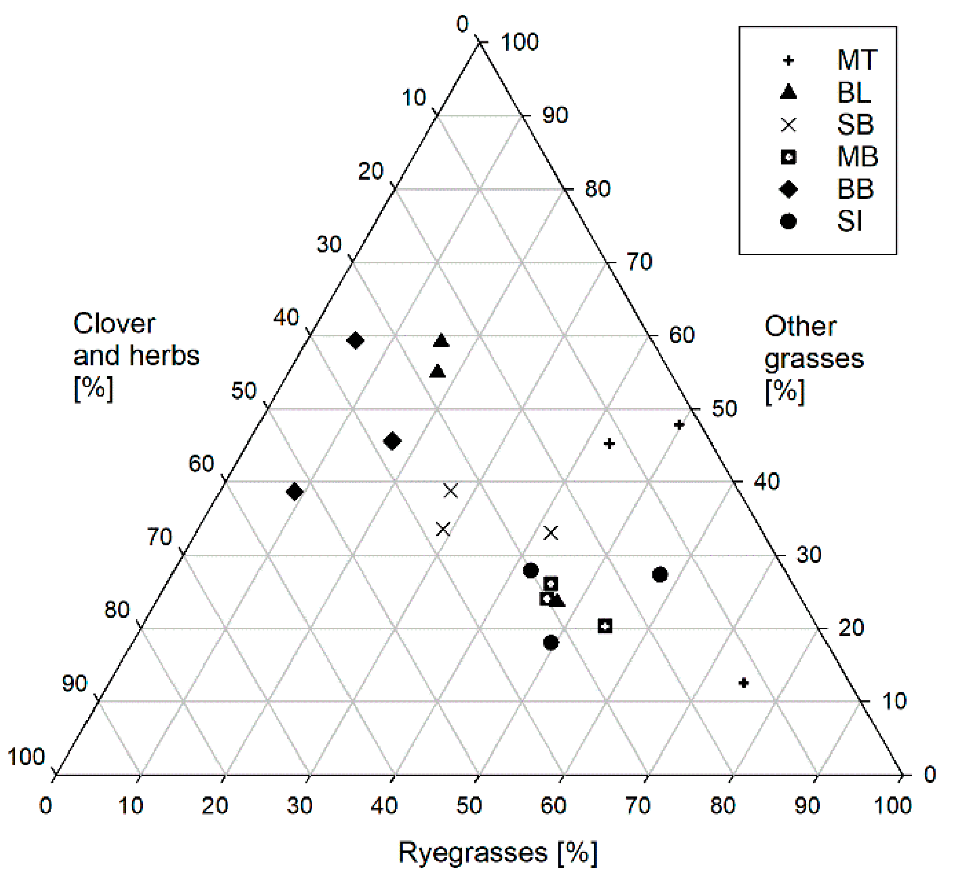
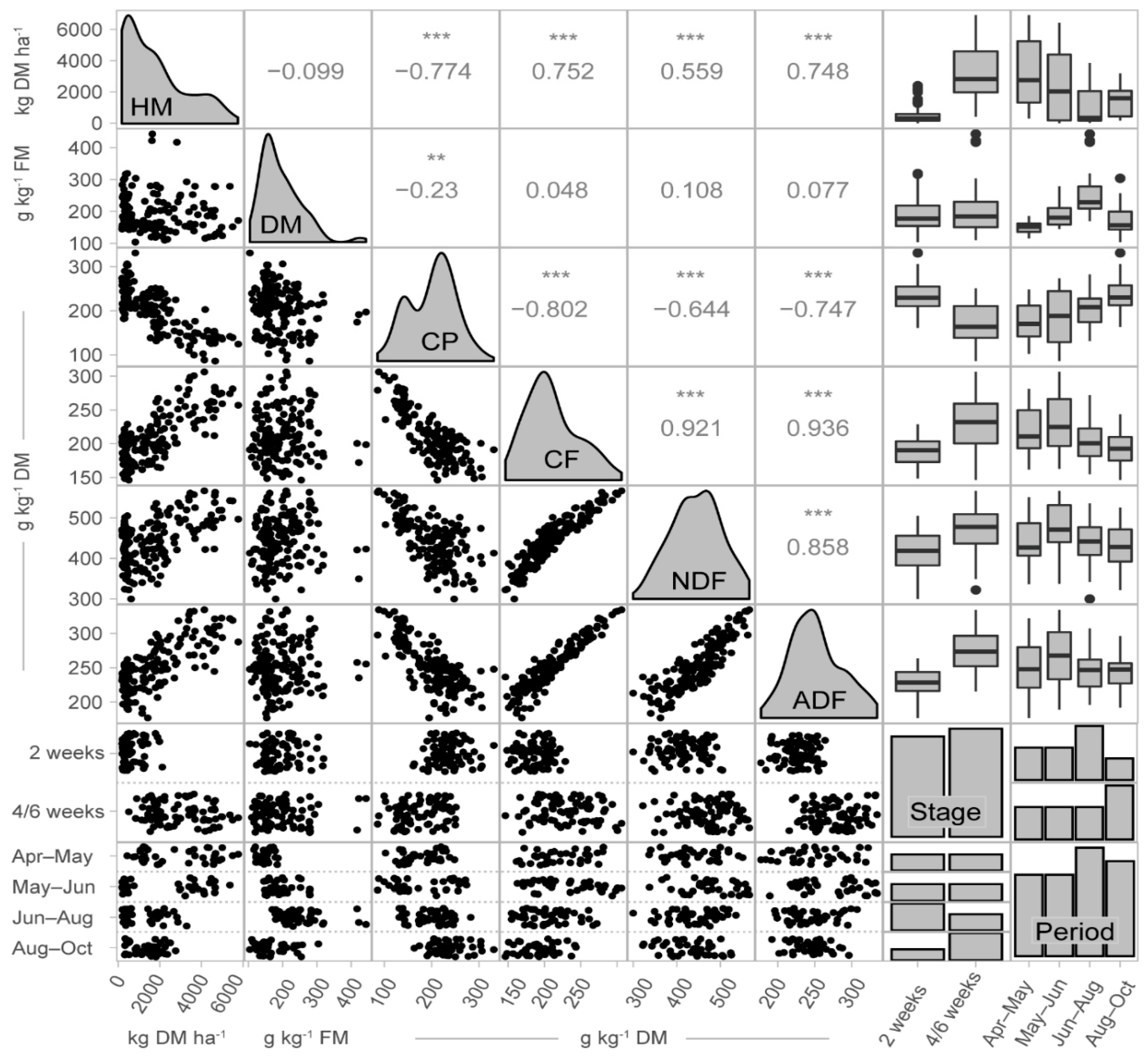
3.2. Sample Characteristics

Figure 3 shows the range of HM and quality parameters as measured with the reference methods (Table 1); the boxplots visualize their distribution, as observed for the two growth stages and the four growth periods, respectively.
Across all measurements, HM ranged from 186 to 5770 kg DM ha−1. The herbage quality ranged from 104 to 443 g DM kg−1 FM and from 86 to 331 g CP kg−1 DM, with structural carbohydrate concentrations from 146 to 306 g CF kg−1 DM, 300 to 567 g NDF kg−1 DM, and 177 to 334 g ADF kg−1 DM. As expected, the average HM for each cut was much higher with the 4/6 weeks defoliation regime than with the two weeks regime (Figure 3, boxplots show the stages). Conversely, the herbage quality was lower in older grasslands, as indicated by the lower CP concentration and the increased concentrations of structural carbohydrates (CF, ADF, and NDF) in the advanced growth stage (4/6 weeks).
CP correlated negatively with HM and with CF, ADF, and NDF (Figure 3). The mean CP increased with progression of the growth period. Conversely, the mean CF, NDF, and ADF concentrations peaked in spring and then decreased as the growth period progressed.

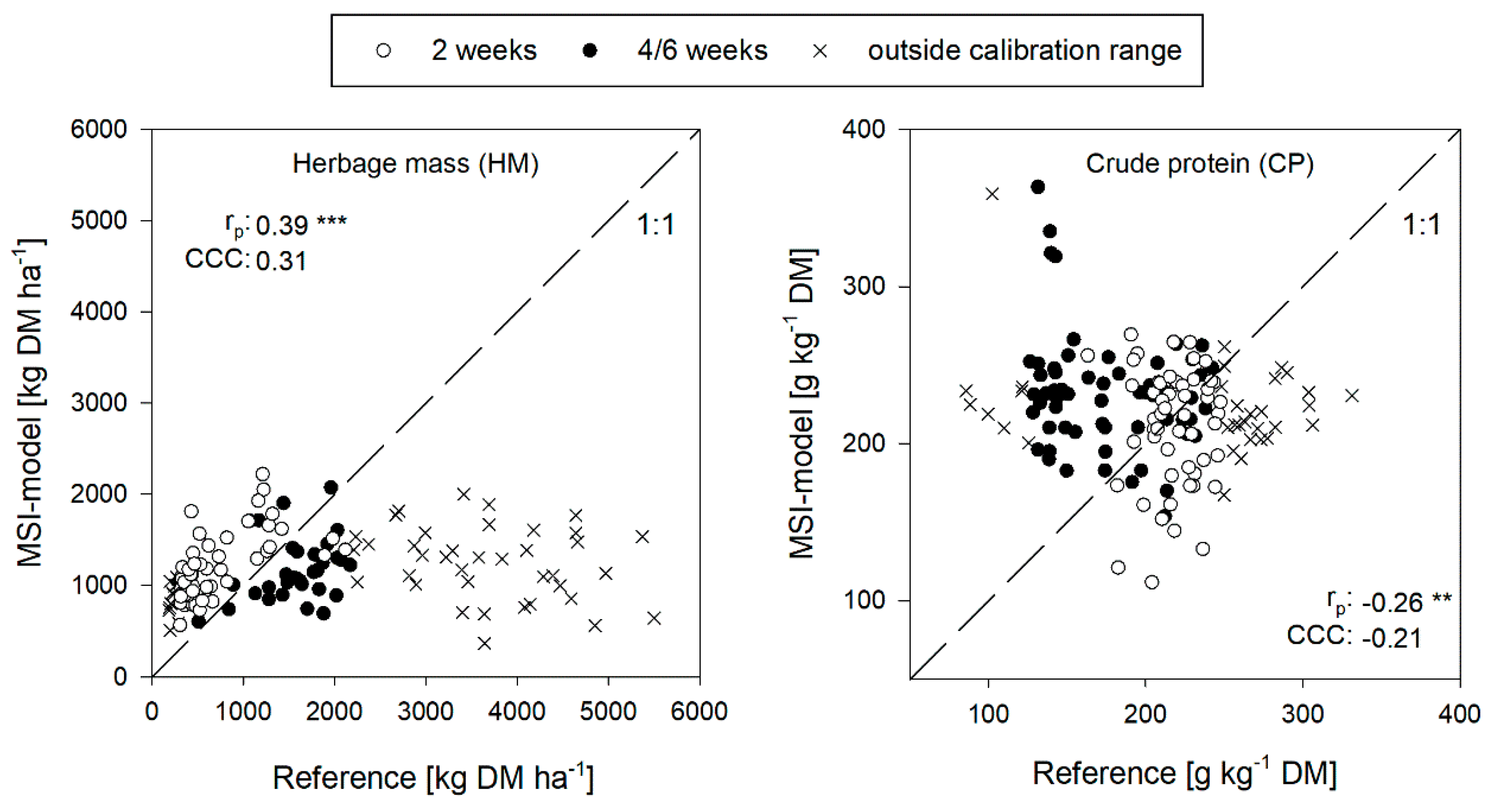
3.3. Performance of the MSI-Model

The MSI-models for determining HM and CP were shown to have poor agreement with the reference method. As shown in Figure 4, we measured a slight concordance between the MSI-model and the reference data for HM (CCC: 0.31, rp: 0.39) and no concordance for CP (CCC: −0.21, rp: −0.26), even though the data outside of the calibration range of the MSI-model was excluded.
Separately considering the two growth stages, we found a slightly higher concordance for the 2-week herbage (n = 62, CCC: 0.35, rp: 0.64) compared to the 4/6-week herbage (n = 36, CCC: 0.21, rp: 0.41) in measuring HM. The HM of the younger herbage (two weeks) was generally overestimated, whereas the older and more mature herbage (4/6 weeks) was mostly underestimated (Figure 4).
Table 3 shows linear models that explain the variation in the observed absolute errors (|reference − MSI-model|) within the calibration range using HM, growth period (four nominal levels), plot (18 nominal levels), and DM. The variation in the errors of the MSI-model, which measures HM and CP within the calibration range, could be explained by 29% and 59%, respectively (R2 in Table 3). The highest contributions to the explained variances in HMerror and CPerror were attributed to the plot variable and HM (HMref), respectively. The variable HMref was positively related to CPerror and HMerror (mathematical sign of the regression coefficient in Table 3). Thus, an increase in HMref was related to the higher error in CP and HM, respectively. The growth period was the second-most important explanatory variable for CPerror.

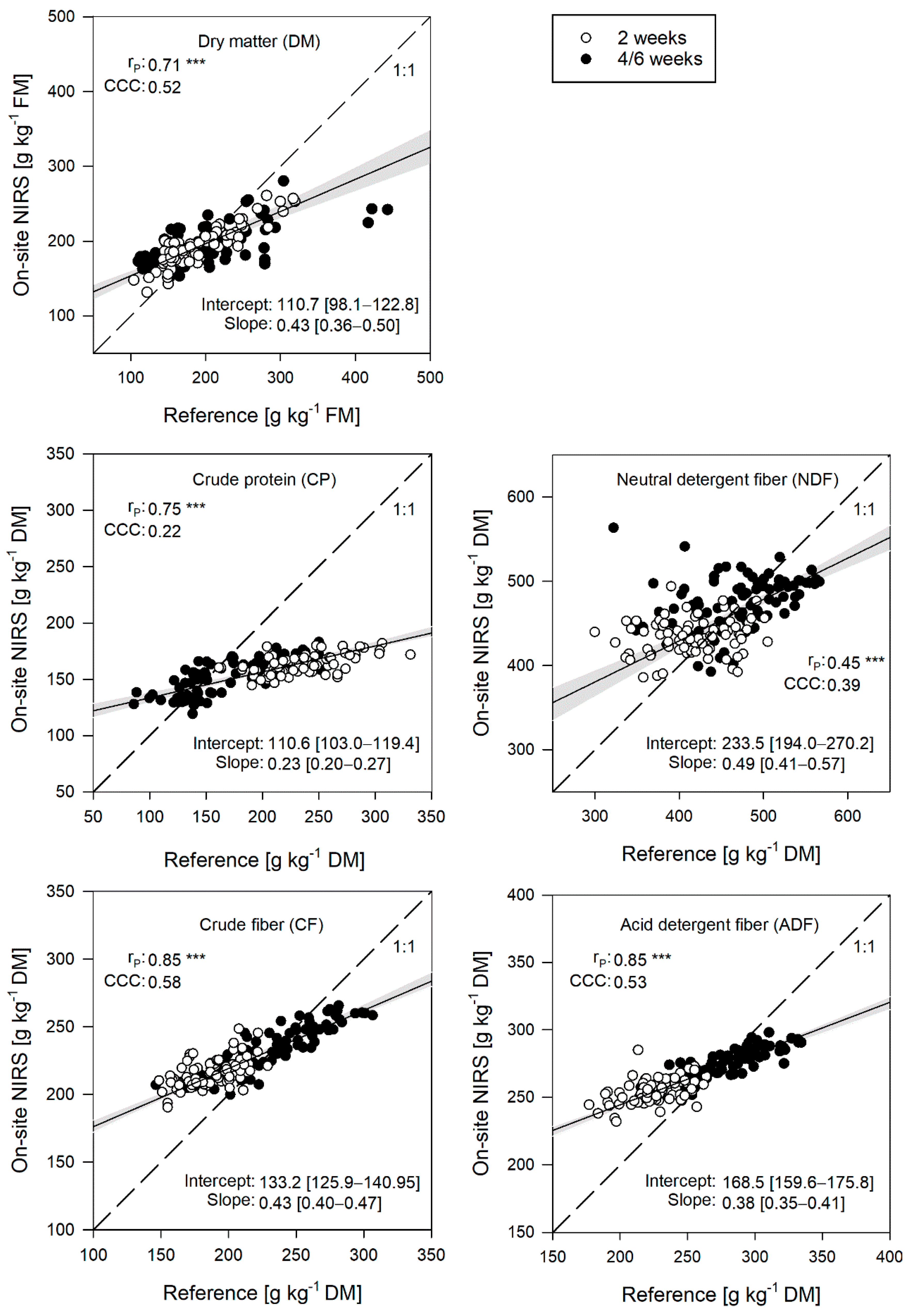
3.4. Performance of the On-Site NIRS

The On-site NIRS determined the fresh herbage quality parameters in large disagreement with the reference methods, oven-drying and the laboratory NIRS (Figure 5). Low concentrations were mostly overestimated, and high concentrations were underestimated. The generally low concordance increased in the order CP < NDF < DM < ADF < CF (CCC: 0.22–0.58). Correlations with the reference were moderate for DM, CP, CF, and ADF (rP: 0.71–0.85) and slight for NDF (rp: 0.45). These results indicate that the random contribution to the error was greater for NDF than for other quality parameters determined by the On-site NIRS. Passing–Bablok regression analysis identified significant systematic errors for all parameters. The confidence intervals of the intercepts and slopes did not include 0 and 1, respectively, which indicates that both a constant and a proportional systematic error was apparent (Figure 5).

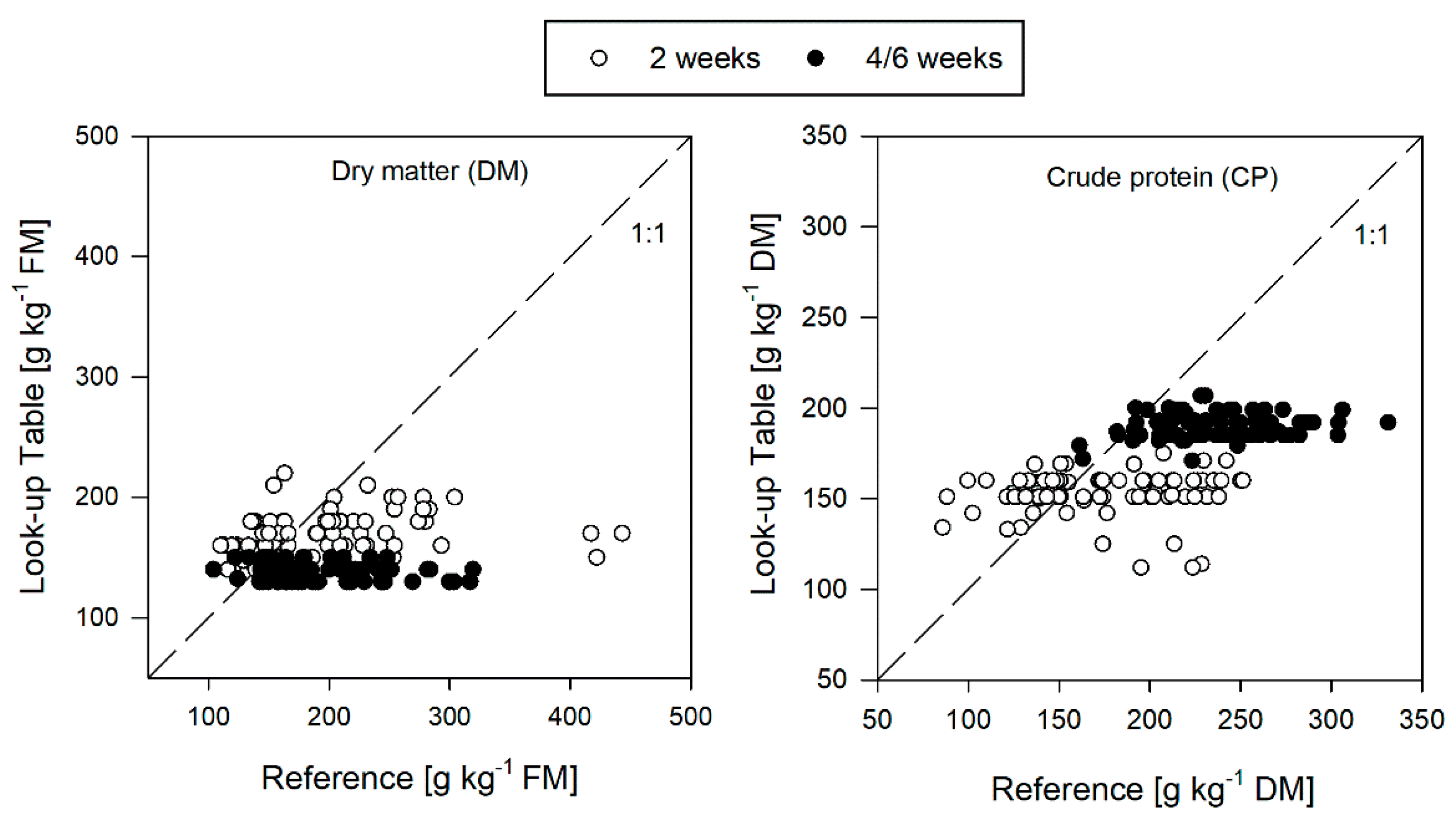
3.5. Performance of the Look-Up Tables

The agreement between the selected herbage parameters DM and CP, which was evaluated using the Look-up Tables and reference measurements, is presented in Figure 6. As expected from the herbage categories available in the Look-up Tables [10], this method clearly differentiated the two growth stages with respect to herbage quality. Nevertheless, the variability in herbage quality within the growth stages was very poorly represented by this method. The herbage quality parameters CF, NDF, and ADF showed similar patterns and are presented in Figure S2.

3.6. Comparison Between Methods

Table 4 compares the performance of all applied methods in HM and quality determination. Absolute and absolute percentage errors are listed, where the latter represents a relative error. The identified systematic error of the On-site NIRS was successfully corrected using two approaches: a correction based on the Passing–Bablok regression that was fitted to the full dataset and fitted in a leave-one-farm-out fashion.
The mean absolute percentage error in measuring the HM and quality decreases in the following order of the determining tools: MSI-model > Look-up Tables ≥ On-site NIRS (Table 4). In determining CP, CF, NDF, and ADF, both the On-site NIRS and the Look-up Tables performed comparably with respect to the relatively large standard deviations. The On-site NIRS determined DM better than the Look-up Tables.
After correcting the systematic error in the On-site NIRS measurement (slopes and intercepts shown in Table S3), the mean absolute percentage errors for quality parameters decreased from 9.3–22.2% to 2.4–7.7% (Table 4). The MSI-model disagreed most with the reference methods presenting mean absolute percentage errors of 99.7% and 33.2% in determining HM and CP, respectively. The measurement errors of the tool decreased when considering only values inside the calibration range (HM: n = 98, CP: n = 113, Figure 4), which reveals absolute percentage errors of 86.3% (HM) and 29.6% (CP) and absolute errors of 562.5 ± 266.6 kg DM ha−1 and 49.0 ± 43.2 g CP kg−1 DM.

4. Discussion

4.1. Generalizability of the MSI-Model

Our results emphasize the importance of a comprehensive evaluation of spectral reflectance-based smart farming tools for determining the HM and grass quality.
The MSI-model was the tool that showed the largest disagreement with the reference measurements (Table 4, Figure 4). Limited generalizability of the model was presumably the main cause for this discrepancy. The model was calibrated with data obtained from a very small range of grassland types. Indeed, all the grasslands that were used for calibration were perennial ryegrass-white clover mixtures (70:30 ratio) in an early growth stage and located within a single research farm [31]. Thus, the calibration dataset ranged to a maximum of 2436 kg DM ha−1 and 247.3 g CP kg−1 DM. These grasslands represent the major grassland type observed on agriculturally managed land in Ireland [39]. Conversely, the great majority of multi-species grasslands that were considered in our study included three to six grass species, with a distinct set of species at different sites, as well as two clover species and three herb species with relative abundances ranging from 1 to 15% and 2 to 48%, respectively. Observed HM ranged to 5770 kg DM ha−1, which is more than double the maximum HM in the calibration data. Less pronounced, CP exceeded the calibration range by 84 g kg−1 DM.
When extrapolating beyond the calibration range in terms of HM and CP values, the MSI-model increasingly failed to accurately determine the HM. Therefore, we analyzed the potential sources of error of the MSI-model for the calibration range only (Table 3). Askari et al. [31], who developed the model, obtained reasonable performance when they validated the models for HM and CP with a subset of their ryegrass-clover mixtures excluded during calibration. Conversely, even considering values within the calibration range only, the model performance was very poor for the Swiss multi-species grasslands of this study. The plot variable, which represents the 18 grasslands that contain the sampled subplots (2 subplots × 5 samples each; Figure 2), was attributable for 83.6% and 15.7% of the explained variance in the errors in HM and CP, respectively. This finding indicates that the discrepancy between the two studies is due to a different and more diverse botanical composition and larger environmental variability in the current study.
Furthermore, the performance of the MSI-model was slightly better for the two-week-grown herbage than for the four-to-six week grown herbage (CCC: 0.35, versus CCC: 0.21). The two-week grown herbage was presumably morphologically more similar to the calibration data representing mainly young and leafy plant biomass, which is typical for grazing conditions. This might explain the better performance. While the described generalizability problem can be overcome with calibration data that better represent the grasslands to which the model will be applied, there are sources of error inherent to the method that need to be addressed differently.

4.2. Difficulty of Remotely Sensing High-Biomass Grasslands by MSI

Remote sensing techniques mainly capture signals from canopy surfaces and increasingly less signals from lower vegetation layers [26,40]. The poor sensing of the lower layers increasingly introduces greater uncertainty in grassland property determination with taller stands and vertical heterogeneity. In our study, the error in determining CP was to a large extent explained by the standing HM, which shows increased error of CP with an increase in HM (Table 3). Consistent with this rational of disproportionately higher sensing of the upper, protein-rich leafy layers compared to that of the lower layers with more low-protein, fiber-rich stems, CP was overestimated at higher standing biomass (Figure S3). The effect of decreasing signal strength from lower vegetation layers can also partially explain the frequently reported asymptotical approaching of a reflectance saturation with increasing biomass or leaf area index [26,41,42]. Other effects, such as decreasing chlorophyll contents when herbage matures might also contribute to this saturation effect [43,44].
The means of the single bands and indices that were used in the MSI-model [31] were calculated for the sampled areas and plotted against HM (Figures S4 and S5). There was a pronounced flattening of the curves at approximately 1300 kg DM ha−1 and low or, in case of the red and green bands, near zero slope at higher HM. The observed missing sensitivity of the MSI-model at high HM was, therefore, likely (co)determined by the saturation effect. Because the saturation effect is more or less pronounced for different wavelengths, selecting less affected bands and vegetation indices for use in models might mitigate the saturation issue [40]. The red-edge narrow band between 730 nm and 740 nm and indices that include red-edge information are particularly suited for this purpose [42]. Multispectral sensors that are designed for vegetation monitoring, such as the Parrot Sequoia sensor, therefore included this band. In stepwise variable selection for the MSI-model, Askari et al. [31] also included indices and bands that are particularly suitable to address the saturation problem, i.e., difference-indices instead of ratio-indices and the green and red-edge band [40,42]. However, the saturation effect might not have had considerable weight toward the selection of variables because the variable selection was based on training data with a limited range in biomass. In case the calibration range of the MSI-model is extended toward higher biomass, a re-selection of the variables might be preferable to a simple recalibration of the model.

4.3. Perspectives of MSI on Grasslands

The grass height can be modelled using structure-from-motion photogrammetry on overlapping aerial images that are taken from different angles [45,46]. Considering such three-dimensional information complementary to the spectral information was shown to enhance the performance of models that determine the HM and nitrogen content [47]. Because the reconstruction of the three-dimensional sward scenery is less affected by spectral saturation, including this information might increase the model performance particularly for grasslands with high biomass. A lot of photogrammetry software incorporates structure-from-motion [48] and can output a digital surface model as a byproduct of the creation of two-dimensional reflectance maps that are needed for using the MSI-model. Subtracting the digital surface model from a digital terrain model, which represents the soil surface, will yield the map with grass height estimates. Incorporation of grass height estimates to improve the MSI-model would, thus, not make the overall workflow for the user more complex but would create the additional requirement of an accurate enough digital terrain model. This information can be obtained with the same structure-from-motion technique during periods of bare soil or very low grass canopy after harvest.

4.4. Improving the Decision Support Platform for Remote Grassland Assessment

The technical realization of how the calibrated model is employed might introduce additional errors. On the GrassQ platform www.grassq.com (as of 2 July 2019), area means are calculated by taking the arithmetic mean of the corresponding HM or CP pixel values. This process will introduce errors for concentrations, such as CP, which are not simply additive but should instead be aggregated as the weighted mean with the biomass distribution as weights. The error that arises from using the arithmetic mean instead of a weighted mean might be reasonably small for very homogeneous grasslands but will rise quickly with increasing heterogeneity and might considerably contribute to the observed error of the MSI-model in this study. On the GrassQ platform, HM and CP are calculated for each pixel of the reflectance data, which in our study represented an area of approximately 5 cm × 5 cm grassland. However, the applied MSI-model was calibrated on a much coarser spatial scale, using mean reflectance values of 1.5 m × 5 m plots [31]. The heterogeneity and range of expected reflectance values is presumably broader across the pixels than the range of mean reflectance values observed on the coarse spatial scale of calibration. For example, pixels that represent bare soil will show reflectance values far beyond the calibration range (of mean values). This may introduce errors when applying the MSI-model to heterogeneous multi-species or thin grassland.

4.5. Potential for Correcting Systematic Errors of the On-Site NIRS

The On-site NIRS showed absolute percentage errors between 9.3% and 22.2% in determining grass quality parameters (Table 4). The relatively low performance was largely due to a systematic error. However, the correlations between the quality parameters and the reference measurements were high (rP ≥ 0.71), except for NDF (rP 0.45, Figure 5). The On-site NIRS generally overestimated low concentrations and underestimated high concentrations (Figure 5). Long et al. [22] determined DM concentrations of alfalfa-grass mixtures using the HarvestLabTM 3000, both as a mobile instrument, same as in this study, and mounted onto a forage harvester. Similar to our study, they observed a high correlation with the DM measurements obtained by oven-drying and identified systematic errors. However, they reported that on average the high DM concentrations were overestimated and the low DM concentrations were underestimated in case of the mobile NIRS application (within the DM range from 213–497 g kg-1 FM). Evaluating three mobile NIRS tools in measuring several grass quality parameters, including DM, CP, and ADF, Patton et al. [23] also observed systematic over- and underestimation.
Instrument response shifts are a known problem in NIRS analysis and have been reported to cause systematic errors [19,49]. A response shift means a difference in wavelength or reflectance measurements by NIRS instruments that occur either after a given operation time or between NIR instruments even if they are technically identical. Response shifts are particularly problematic when transferring NIR calibrations from one instrument to another, for example when producing instruments in quantity. The systematic errors identified in our study are likely explained by these shifts. To address this problem, Long et al. [22] proposed performing frequent wavelength standard measurements via the HarvestLabTM 3000 software, a process that is typically conducted during maintenance service. Chen et al. [50] suggested a simple method for correcting response differences between instruments using a few standardization samples. In our study, the remaining error of the On-site NIRS after correction of the systematic error using the Passing–Bablok linear regression was ≤ 7.7% (Table 4). This remaining error is surprisingly small, in particular for a mobile instrument employed outside controlled laboratory conditions and using a calibration that does not differentiate grassland types. To put this finding in perspective, relative differences in the range of 3.8% (NDF) to 5.2% (CP) were observed between well-established laboratory NIRS with calibration tailored for Swiss grasslands and wet-chemical analyses (Figure S1).
The remaining error might partially be caused by limited generalizability to grasslands that are not well represented by the calibration [17]. The question has been raised whether NIRS calibrations should be global or developed for local or plant family- and species-specific applications [51,52]. Interregional calibrations have been successfully employed on dried herbage and were found to be robust when grassland characteristics were similar to the calibration data [17,51]. However, our results indicate that calibrations might not need to be grassland-type-specific. Certainly, some error could be reduced by sample preparation processes, such as the processes performed for laboratory NIRS analyses i.e., homogenizing of the plant material by drying and milling [19]. However, the saving of these working processes renders the mobile NIRS attractive for farmers in the first place, because it enables near real-time results to be obtained on-farm [6].

4.6. Benefits of Smart Farming Tools

Until aerial MSI for grassland assessment supersedes conventional approaches, such as look-up tables or costly laboratory analyses, methods such as the MSI-model still need to be intensively developed. However, the On-site NIRS performed equally well than the Look-up Tables by Daccord et al. [10] and even substantially better after correction of the systematic error (Table 4). Unlike the Look-up Tables, the On-site NIRS was able to detect seasonal and short-term variation in grassland quality in our study (analysis not shown). In particular, the parameter DM, which reacts to recent weather conditions, was better captured by the On-site NIRS. Besides the better temporal resolution, the On-site NIRS does not require any botanical knowledge. Compared to the laboratory analysis, farmers receive results in a timely manner, which is a clear advantage over sending samples to a commercial laboratory with similar accuracy.

5. Conclusions

The two smart farming tools for grassland assessment evaluated in this study were in different development stages. The smart farming tool that is based on a model for analyzing MSI performed worse regarding grass quality assessment than the conventional Look-up Tables but showed potential in estimating HM on grasslands with low biomass, i.e., in situations that often pertain to grazing management. It was identified that the saturation of reflectance indices is likely to limit the performance for high-biomass grasslands, and evidence was obtained that indicates that the model performance was co-determined by grassland characteristics. Further model development might focus on extending the calibration dataset with respect to spatiotemporal diversity and include three-dimensional information, such as grass height, to mitigate limitations due to saturating reflectance. The second smart farming tool, the On-site NIRS, performed better or comparable to the Look-up Tables. We found that the error for the On-site NIRS was mainly systematic, and therefore, predictable and correctable, indicating great potential of the On-site NIRS to become a tool that is accurate enough for practical use by farmers in the near future.

Supplementary Materials

The following are available online at https://www.mdpi.com/2072-4292/12/19/3256/s1, Table S1 Characteristics of studied grasslands and observations.; Table S2 Characteristics of the calibration model of the laboratory NIRS (Fourier-Transform NIR, N-500, Büchi, Flawil, Switzerland; all herbage parameters as g kg−1 DM).; Table S3 Passing–Bablok regression result from fitting the full dataset or fitting five of six farms (left-out farm indicated).; Figure S1 Laboratory NIRS measurements versus the validation methods (n = 54, Table 2) for quality parameters in dried herbage. Dashed line is the line of identity (1:1). The open and filled dots represent the two growth stages of the plants: “2 weeks” of growth and “4/6 weeks” of growth. The values of Pearson’s correlation coefficient (rP), Lin’s concordance correlation coefficient (CCC), and the mean absolute percentage error (MAPE) are given. CA was not further used to evaluate smart farming tools in the study, because sampling was prone to soil contamination. Data points far from the line of identity were confirmed to not explain measurement errors of other parameters.; Figure S2 Herbage quality parameters determined with the Look-up Tables by Daccord et al. [10] versus the reference methods (n = 162). The dashed line is the line of identity (1:1). The open and filled dots represent the two growth stages of the plants: “2 weeks” of growth and “4/6 weeks” of growth.; Figure S3 The error of the MSI-model (reference − MSI-model) in determining crude protein (CP) versus the herbage mass (n = 147). The open and filled dots represent the two growth stages of the plants: “2 weeks” growth and “4/6 weeks” of growth.; Figure S4 Reflectance in four spectral bands determined by UAV multispectral imagery versus the herbage mass (n = 147). Values are plot-area means of the corresponding pixel values. Solid line is a smooth LOESS trend line. The open and filled dots represent the two growth stages of the plants: “two weeks” of growth and “4/6 weeks” of growth. Nine and one far outlying data points are not shown for red-edge and red, respectively.; Figure S5 Vegetation indices determined by UAV multispectral imagery versus the herbage mass (n = 147). Values are plot-area means of pixel-wise calculate indices. The solid line is a smooth LOESS trend line. The open and filled dots represent the two growth stages of the plants: “2 weeks” of growth and “4/6 weeks” of growth. The plot for MCAR does not show nine far outlying data points. Abbreviation of indices: SR5: Single Ratio 5; MCAR: Modified Chlorophyll Absorption Ratio; SR3: Single Ratio 3. Definition of indices according to Askari et al. [31].

Author Contributions

Conceptualization, L.H., R.L., and C.U.; Data curation, L.H.; Formal analysis, L.H. and M.S.; Funding acquisition, C.U.; Investigation, L.H. and O.H.-E.; Methodology, L.H., O.H.-E., R.L., and S.D.; Project administration, C.U.; Resources, O.H.-E. and C.U.; Software, L.H. and M.S.; Supervision, R.L. and C.U.; Validation, L.H., O.H.-E., and C.U.; Visualization, L.H. and M.S.; Writing—original draft, L.H.; Writing—review and editing, L.H., O.H.-E., R.L., M.S., S.D., and C.U. All authors have read and agreed to the published version of the manuscript.

Funding

This research was funded by the Swiss Federal Office for Agriculture within the project “GrassQ” under the ICT-Agri ERA-Net Call “Enabling Precision Agriculture”, Project ID 35779.

Acknowledgments

We gratefully acknowledge the possibility to use the experimental design of a larger Swiss study with experimental plots established and managed by the research group for forage production and grassland (Agroscope, Switzerland). We thank Rafael Gago and Cornel Stutz for their dedication during fieldwork.

Conflicts of Interest

The authors declare no conflict of interest. The funders had no role in the design of the study; in the collection, analyses, or interpretation of data; in the writing of the manuscript, or in the decision to publish the results.

References

  1. Beaver, A.; Ritter, C.; von Keyserlingk, M.A.G. The Dairy Cattle Housing Dilemma: Natural Behavior Versus Animal Care. Vet. Clin. N. Am. Food A 2019, 35, 11–27. [Google Scholar]
  2. Van den Pol-van Dasselaar, A.; de Vliegher, A.; Hennessy, D.; Peyraud, J.L.; Pinxterhuis, J.B. Research Methodology of Grazing; Wageningen UR Livestock Research: Lelystad, The Netherlands, 2011. [Google Scholar]
  3. Rutter, S.M. Can precision farming technologies be applied to grazing management. In Revitalising Grasslands to Sustain Our Communities, Proceedings of 22nd International Grassland Congress, Sydney, Australia, 15–19 September 2013; Michalk, D.L., Millar, G.D., Eds.; New South Wales Department of Primary Industry: Orange, New South Wales, Australia, 2013; pp. 617–620. [Google Scholar]
  4. Turner, L.; Irvine, L.; Kilpatrick, S. Incorporating data into grazing management decisions: Supporting farmer learning. Anim. Prod. Sci. 2020, 60, 138–142. [Google Scholar] [CrossRef]
  5. Ferraro, F.P.; Nave, R.L.G.; Sulc, R.M.; Barker, D.J. Seasonal Variation in the Rising Plate Meter Calibration for Forage Mass. Agron. J. 2012, 104, 1–6. [Google Scholar] [CrossRef]
  6. Bell, M.J.; Mereu, L.; Davis, J. The Use of Mobile Near-Infrared Spectroscopy for Real-Time Pasture Management. Front. Sustain. Food Syst. 2018, 2, 76. [Google Scholar] [CrossRef] [Green Version]
  7. Calanca, P.; Deléglise, C.; Martin, R.; Carrère, P.; Mosimann, E. Testing the ability of a simple grassland model to simulate the seasonal effects of drought on herbage growth. Field Crop. Res. 2016, 187, 12–23. [Google Scholar] [CrossRef]
  8. Le Clec’h, S.; Finger, R.; Buchmann, N.; Gosal, A.S.; Hörtnagl, L.; Huguenin-Elie, O.; Jeanneret, P.; Lüscher, A.; Schneider, M.K.; Huber, R. Assessment of spatial variability of multiple ecosystem services in grasslands of different intensities. J. Environ. Manag. 2019, 251, 109372. [Google Scholar] [CrossRef] [PubMed]
  9. Lile, J.A.; Blackwell, M.B.; Thomson, N.A.; Penno, J.W.; Macdonald, K.A.; Nicholas, P.K.; Lancaster, J.A.S.; Coulter, M. Practical Use of the Rising Plate Meter (RPM) on New Zealand Dairy Farms. In Proceedings of the NZ Grassland Association, Hamilton, New Zealand, 6–8 November 2001; NZ Grassland Association Inc.: Dunedin, New Zealand, 2001; Volume 63, pp. 159–164. [Google Scholar]
  10. Daccord, R.; Wyss, U.; Kessler, J.; Arrigo, Y.; Rouel, M.; Lehmann, J.; Jeangros, B.; Meisser, M. Nutritional value of roughage. In Feed Recommendations for Ruminants (Green Book); Daccord, R., Wyss, U., Eds.; Agroscope: Posieux, Switzerland, 2017. [Google Scholar]
  11. Deléglise, C.; Meisser, M.; Mosimann, E.; Spiegelberger, T.; Signarbieux, C.; Jeangros, B.; Buttler, A. Drought-induced shifts in plants traits, yields and nutritive value under realistic grazing and mowing managements in a mountain grassland. Agric. Ecosyst. Environ. 2015, 213, 94–104. [Google Scholar] [CrossRef]
  12. Michaud, A.; Plantureux, S.; Pottier, E.; Baumont, R. Links between functional composition, biomass production and forage quality in permanent grasslands over a broad gradient of conditions. J. Agric. Sci. 2015, 153, 891–906. [Google Scholar] [CrossRef]
  13. Peratoner, G.; Kasal, A.; Florian, C.; Pramsohler, M. Accuracy of visual assessment of the plant stand type for the estimation of forage quality. Grassl. Sci. Eur. 2018, 23, 950–952. [Google Scholar]
  14. Pullanagari, R.R.; Yule, I.; King, W.; Dalley, D.; Dynes, R. The use of optical sensors to estimate pasture quality. Int. J. Smart Sens. Intell. Syst. 2011, 4, 125–137. [Google Scholar] [CrossRef] [Green Version]
  15. Lugassi, R.; Chudnovsky, A.; Zaady, E.; Dvash, L.; Goldshleger, N. Spectral Slope as an Indicator of Pasture Quality. Remote Sens. 2015, 7, 256–274. [Google Scholar] [CrossRef] [Green Version]
  16. Norris, K.H.; Barnes, R.F.; Moore, J.E.; Shenk, J.S. Predicting Forage Quality by Infrared Replectance Spectroscopy. J. Anim. Sci. 1976, 43, 889–897. [Google Scholar] [CrossRef]
  17. Mika, V.; Pozdisek, J.; Tillmann, P.; Nerusil, P.; Buchgraber, K.; Gruber, L. Development of NIR calibration valid for two different grass sample collections. Czech J. Anim. Sci. 2003, 48, 419–424. [Google Scholar]
  18. Alomar, D.; Fuchslocher, R.; Cuevas, J.; Mardones, R.; Cuevas, E. Prediction of the composition of fresh pastures by near infrared reflectance or interactance-reflectance spectroscopy. Chil. J. Agric. Res. 2009, 69, 198–206. [Google Scholar] [CrossRef] [Green Version]
  19. Soldado, A.; Fearn, T.; Martinez-Fernandez, A.; de la Roza-Delgado, B. The transfer of NIR calibrations for undried grass silage from the laboratory to on-site instruments: Comparison of two approaches. Talanta 2013, 105, 8–14. [Google Scholar] [CrossRef] [PubMed]
  20. Harris, P.A.; Nelson, S.; Carslake, H.B.; Argo, C.M.; Wolf, R.; Fabri, F.B.; Brolsma, K.M.; van Oostrum, M.J.; Ellis, A.D. Comparison of NIRS and Wet Chemistry Methods for the Nutritional Analysis of Haylages for Horses. J. Equine Vet. Sci. 2018, 71, 13–20. [Google Scholar] [CrossRef]
  21. Ampuero Kragten, S.; Wyss, U. Feedstuff in near infrared light (NIRS). Agrar. Schweiz 2014, 5, 204–211. [Google Scholar]
  22. Long, E.A.; Ketterings, Q.M.; Russell, D.; Vermeylen, F.; DeGloria, S. Assessment of yield monitoring equipment for dry matter and yield of corn silage and alfalfa/grass. Precis. Agric. 2016, 17, 546–563. [Google Scholar] [CrossRef]
  23. Patton, L.; McConnell, D.; Archer, J.; O’Donovan, M.; Gilliland, T.J. Portable NIRS: A novel technology for the prediction of forage nutritive quality. Grassl. Sci. Eur. 2018, 23, 892–894. [Google Scholar]
  24. Berzaghi, P.; Marchesini, G. Rapid Methods of Analysis of Silages to Improve Feeding Management in Dairy Farms. In Proceedings of the 16th International Symposium Forage Conservation, Brno, Czech Republic, 3–6 June 2014; Jambor, V., Malá, S., Eds.; Mendel University: Brno, Czech Republic, 2014; pp. 65–70. [Google Scholar]
  25. Rueda-Ayala, V.P.; Peña, J.M.; Höglind, M.; Bengochea-Guevara, J.M.; Andújar, D. Comparing UAV-Based Technologies and RGB-D Reconstruction Methods for Plant Height and Biomass Monitoring on Grass Ley. Sensors 2019, 19, 535. [Google Scholar] [CrossRef] [PubMed] [Green Version]
  26. Wachendorf, M.; Fricke, T.; Möckel, T. Remote sensing as a tool to assess botanical composition, structure, quantity and quality of temperate grasslands. Grass Forage Sci. 2018, 73, 1–14. [Google Scholar] [CrossRef]
  27. Iftikhar, A.; Cawkwell, F.; Dwyer, E.; Barrett, B.; Green, S. Satellite remote sensing of grasslands: From observation to management. J. Plant. Ecol. 2016, 9, 649–671. [Google Scholar] [CrossRef] [Green Version]
  28. Bareth, G.; Schellberg, J. Replacing Manual Rising Plate Meter Measurements with Low-cost UAV-Derived Sward Height Data in Grasslands for Spatial Monitoring. PFG J. Photogramm. Rem. 2018, 86, 157–168. [Google Scholar] [CrossRef]
  29. Aasen, H.; Honkavaara, E.; Lucieer, A.; Zarco-Tejada, P.J. Quantitative Remote Sensing at Ultra-High Resolution with UAV Spectroscopy: A Review of Sensor Technology, Measurement Procedures, and Data Correction Workflows. Remote Sens. 2018, 10, 1091. [Google Scholar] [CrossRef] [Green Version]
  30. Murphy, D.; O‘Brien, B.; Askari, M.S.; McCarthy, T.; Magee, A.; Burke, R.; Murphy, M. GrassQ—A Holistic Precision Grass Measurement and Analysis System to Optimize Pasture Based Livestock Production. In Proceedings of the 2019 ASABE Annual International Meeting, Boston, MA, USA, 7–10 July 2019; ASABE: St. Joseph, MA, USA, 2019; p. 1900769. [Google Scholar]
  31. Askari, M.S.; McCarthy, T.; Magee, A.; Murphy, D.J. Evaluation of Grass Quality under Different Soil Management Scenarios Using Remote Sensing Techniques. Remote Sens. 2019, 11, 1835. [Google Scholar] [CrossRef] [Green Version]
  32. VDLUFA. The chemical analysis of feedstuffs. In VDLUFA Method Book III, 8th ed.; VDLUFA-Verlag: Darmstadt, Germany, 1976; ISBN 978-3-941273-14-6. [Google Scholar]
  33. Lin, L.I. A Concordance Correlation Coefficient to Evaluate Reproducibility. Biometrics 1989, 48, 255–268. [Google Scholar] [CrossRef]
  34. Lindemann, R.H.; Merenda, P.F.; Gold, R.Z. Introduction to Bivariate and Multivariate Analysis; Scott Foresman and Company: Glenview, IL, USA, 1980. [Google Scholar]
  35. Passing, H.; Bablok, W. A new biometrical procedure for testing the equality of measurements from two different analytical methods. Application of linear regression procedures from method comparison studies in clinical chemistry, Part I. J. Clin. Chem. Clin. Biochem. 1983, 21, 709–720. [Google Scholar] [CrossRef] [PubMed]
  36. Stevenson, M. epiR: Tools for the Analysis of Epidemiological Data. Available online: https://CRAN.R-project.org/package=epiR (accessed on 24 February 2020).
  37. Manuilova, E.; Schuetzenmeister, A.; Model, F. mcr: Method Comparison Regression. Available online: https://CRAN.R-project.org/package=mcr (accessed on 3 March 2020).
  38. Grömping, U. Relative Importance for Linear Regression in R: The Package relaimpo. J. Stat. Softw. 2006, 17, 1–27. [Google Scholar] [CrossRef] [Green Version]
  39. O‘Neill, F.H.; Martin, J.R.; Devaney, F.M.; Perrin, P.M. The Irish semi-natural grasslands survey 2007–2012. In Irish Wildlife Manual No. 78; National Parks and Wildlife Service, Department of Arts, Heritage and Gaeltacht: Dublin, Ireland, 2013. [Google Scholar]
  40. Thenkabail, P.S.; Smith, R.B.; de Pauw, E. Hyperspectral Vegetation Indices and Their Relationships with Agricultural Crop Characteristics. Remote Sens. Environ. 2000, 71, 158–182. [Google Scholar] [CrossRef]
  41. Svinurai, W.; Hassen, A.; Tesfamariam, E.; Ramoelo, A. Performance of ratio-based, soil-adjusted and atmospherically corrected multispectral vegetation indices in predicting herbaceous aboveground biomass in a Colophospermum mopane tree–shrub savanna. Grass Forage Sci. 2018, 73, 727–739. [Google Scholar] [CrossRef]
  42. Mutanga, O.; Skidmore, A.K. Narrow band vegetation indices overcome the saturation problem in biomass estimation. Int. J. Remote Sens. 2004, 25, 3999–4014. [Google Scholar] [CrossRef]
  43. Todd, S.W.; Hoffer, R.M.; Milchunas, D.G. Biomass estimation on grazed and ungrazed rangelands using spectral indices. Int. J. Remote Sens. 1998, 19, 427–438. [Google Scholar] [CrossRef]
  44. Zeng, L.; Chen, C. Using remote sensing to estimate forage biomass and nutrient contents at different growth stages. Biomass Bioenergy 2018, 115, 74–81. [Google Scholar] [CrossRef]
  45. Grüner, E.; Astor, T.; Wachendorf, M. Biomass Prediction of Heterogeneous Temperate Grasslands Using an SfM Approach Based on UAV Imaging. Agronomy 2019, 9, 54. [Google Scholar] [CrossRef] [Green Version]
  46. Forsmoo, J.; Anderson, K.; Macleod, C.J.; Wilkinson, M.E.; Brazier, R. Drone-based structure-from-motion photogrammetry captures grassland sward height variability. J. Appl. Ecol. 2018, 55, 2587–2599. [Google Scholar]
  47. Näsi, R.; Viljanen, N.; Kaivosoja, J.; Alhonoja, K.; Hakala, T.; Markelin, L.; Honkavaara, E. Estimating Biomass and Nitrogen Amount of Barley and Grass Using UAV and Aircraft Based Spectral and Photogrammetric 3D Features. Remote Sens. 2018, 10, 1082. [Google Scholar] [CrossRef] [Green Version]
  48. Forsmoo, J.; Anderson, K.; Macleod, C.J.A.; Wilkinson, M.E.; DeBell, L.; Brazier, R.E. Structure from motion photogrammetry in ecology: Does the choice of software matter? Ecol. Evol. 2019, 9, 12964–12979. [Google Scholar] [CrossRef] [PubMed]
  49. Fearn, T. Standardisation and Calibration Transfer for near Infrared Instruments: A Review. J. Near Infrared Spec. 2001, 9, 229–244. [Google Scholar] [CrossRef]
  50. Chen, Z.-P.; Li, L.-M.; Yu, R.-Q.; Littlejohn, D.; Nordon, A.; Morris, J.; Dann, A.S.; Jeffkins, P.A.; Richardson, M.D.; Stimpson, S.L. Systematic prediction error correction: A novel strategy for maintaining the predictive abilities of multivariate calibration models. Analyst 2011, 136, 98–106. [Google Scholar] [CrossRef] [PubMed]
  51. Andueza, D.; Picard, F.; Jestin, M.; Andrieu, J.; Baumont, R. NIRS prediction of the feed value of temperate forages: Efficacy of four calibration strategies. Animal 2011, 5, 1002–1013. [Google Scholar] [CrossRef] [PubMed] [Green Version]
  52. Cougnon, M.; van Waes, C.; Dardenne, P.; Baert, J.; Reheul, D. Comparison of near infrared reflectance spectroscopy calibration strategies for the botanical composition of grass-clover mixtures. Grass Forage Sci. 2013, 69, 167–175. [Google Scholar] [CrossRef]
Figure 1. Relative abundance of ryegrasses, other grasses, and clover and herbs in the 18 studied grasslands, which were distributed over six commercial farms (MT, BL, SB, MB, BB, and SI). The values are the average values from the botanical surveys in spring and late summer 2018.
Remotesensing 12 03256 g001
Figure 2. Selected experimental plot, shown as (a) front view and (b) aerial view, where the dashed lines indicate the two subplots. The sampling areas are highlighted with a checkered pattern. The age of the herbage at sampling was two weeks (left subplot) and four to six weeks (right subplot). The ground control points are highlighted as crossed circles.
Remotesensing 12 03256 g002
Figure 3. Pairs plot of the reference data (oven-drying and laboratory NIRS, n = 162), the growth stage (two weeks and four to six weeks of growth), and the growth period. The herbage parameters are abbreviated as follows: HM: herbage mass, DM: dry matter, CP: crude protein, CF: crude fiber, NDF: neutral detergent fiber, and ADF: acid detergent fiber. The plots in the diagonal line are density plots that show the distribution of the data. The values of Pearson correlation coefficients and the boxplots are shown above the diagonal. Significance codes: *** ≤ 0.001, ** ≤ 0.01.
Remotesensing 12 03256 g003
Figure 4. MSI-model versus reference measurements (n = 147) of HM and CP concentration in herbage. The dashed line is the line of identity (1:1). The open and filled dots represent the two growth stages of the plants: two weeks and four to six weeks of growth. The values of Pearson’s correlation coefficient (rP) and Lin’s concordance correlation coefficient (CCC) were calculated for values inside the calibration range (HM: n = 98, CP: n = 113). Significance codes: *** ≤ 0.001, ** ≤ 0.01.
Remotesensing 12 03256 g004
Figure 5. On-site NIRS versus reference measurements (n = 162) of herbage quality parameters. The dashed line is the line of identity (1:1). The open and filled dots represent the two growth stages of the plants: two weeks of growth and four to six weeks of growth. Passing–Bablok regression is shown as a solid line with a 95% confidence band. Intercept and slope with 95% confidence intervals are indicated. The values of Pearson’s correlation coefficient (rP) and Lin’s concordance correlation coefficient (CCC) are also given. Significance codes: *** ≤ 0.001.
Remotesensing 12 03256 g005
Figure 6. Herbage quality parameters determined with the Look-up Tables by Daccord et al. [10] versus the reference measurements (n = 162). The dashed line is the line of identity (1:1). The open and filled dots represent the two growth stages of the plants: two weeks and four to six weeks of growth.
Remotesensing 12 03256 g006
Table 1. Evaluated smart farming tools and determined herbage parameters with the respective reference methods.
Measurement Tools (Number of Samples)Sensing MethodMeasured Herbage Parameters [Unit]Reference Methods
MSI-model
(n = 147)
MSI of the bands green, red, red-edge, and NIRHM [kg DM ha−1]Cutting defined area + oven-drying
CP [g kg−1 DM]Laboratory NIRS
On-site NIRS
(n = 162)
NIRS with diode arrayDM [g kg−1 FM]Oven-drying
CP [g kg−1 DM]Laboratory NIRS
CF [g kg−1 DM]Laboratory NIRS
NDF [g kg−1 DM]Laboratory NIRS
ADF [g kg−1 DM]Laboratory NIRS
MSI: multispectral imagery; NIRS: near-infrared reflectance spectroscopy; NIR: near-infrared; HM: herbage mass; DM: dry matter; FM: fresh matter; CP: crude protein; CF: crude fiber; NDF: neutral detergent fiber; ADF: acid detergent fiber.
Table 2. Herbage parameters determined by the laboratory NIRS with the respective wet-chemical methods for validation.
Measurement System (Number of Samples)Sensing MethodMeasured Herbage Parameters [Unit]Validation Methods
Laboratory NIRS
(n = 54)
Fourier-transform NIRSCP [g kg−1 DM]Dumas method
CF [g kg−1 DM]Gravimetric analysis
NDF [g kg−1 DM]Gravimetric analysis
ADF [g kg−1 DM]Gravimetric analysis
NIRS: near-infrared reflectance spectroscopy; DM: dry matter; CP: crude protein; CF: crude fiber; NDF: neutral detergent fiber; ADF: acid detergent fiber.
Table 3. Linear models that explain errors of the MSI-model in determining fresh HM and CP concentration within the calibration range of the MSI-model (error = |reference − MSI-model|; HM: n = 98; CP: n = 113).
Response VariablesExplanatory VariablesR2Significance When Added Last §Relative Importance [% of R2] (Mathematical Sign of Regression Coefficient °)
HMerrorHMref0.290.093 (*) 7.3 (+)
growth period 0.5815.9
plot0.10183.6
DMref0.2223.2 (+)
CPerrorHMref0.59<0.000 ***63.8 (+)
growth period 0.004 **18.3
plot0.163 15.7
DMref0.1172.3 (+)
HM: herbage mass; DM: dry matter concentration; CP: crude protein concentration; ref: reference data; § Significance codes: *** ≤ 0.001, ** ≤ 0.01, (*) ≤ 0.1; ° Mathematical sign of regression coefficient given for continuous variables only.
Table 4. Disagreement (mean ± standard deviation) of Look-up Tables, On-site NIRS, and MSI-model with the reference methods (oven-drying and laboratory NIRS; n = 162).
Herbage ParameterLook-Up Tables °On-Site NIRSOn-Site NIRS Corrected *On-Site NIRS Corrected with LOFO MSI-Model
Absolute error§:
HM (kg DM ha−1)----1043.1 ± 1003.1
DM (g kg−1 FM)51.0 ± 49.532.1 ± 31.114.7 ± 13.015.0 ± 13.1-
CP (g kg−1 DM)41.4 ± 30.149.1 ± 33.77.5 ± 5.47.7 ± 5.454.4 ± 45.2
CF (g kg−1 DM)29.5 ± 23.323.0 ± 15.37.1 ± 5.47.5 ± 5.6-
NDF (g kg−1 DM)53.9 ± 41.241.0 ± 33.724.8 ± 22.126.6 ± 22.9-
ADF (g kg−1 DM)27.4 ± 22.421.8 ± 15.85.8 ± 4.86.0 ± 5.0-
Absolute percentage error#:
HM (%)----99.7 ± 84.9
DM (%)23.2 ± 15.216.9 ± 13.67.7 ± 6.17.9 ± 6.1-
CP (%)19.6 ± 12.722.2 ± 12.24.1 ± 3.44.2 ± 3.433.2 ± 39.1
CF (%)14.4 ± 11.712.0 ± 9.53.5 ± 2.83.7 ± 2.9-
NDF (%)11.7 ± 8.59.9 ± 9.85.9 ± 6.06.3 ± 6.2-
ADF (%)10.8 ± 8.59.3 ± 7.82.4 ± 2.12.5 ± 2.2-
° Daccord et al. [10]; * Correction of the systematic error based on Passing–Bablok regression fitted to the full dataset (Figure 5; coefficients in Table S3); Correction of the systematic error based on Passing–Bablok regression fitted in leave-one-farm-out fashion (coefficients in Table S3); n = 147 due to 15 missing values; § |reference − comparison method|; # |(reference − comparison method) × reference−1|.

