Benefit Evaluation of PV Orientation for Individual Residential Consumers


Abstract
1. Introduction
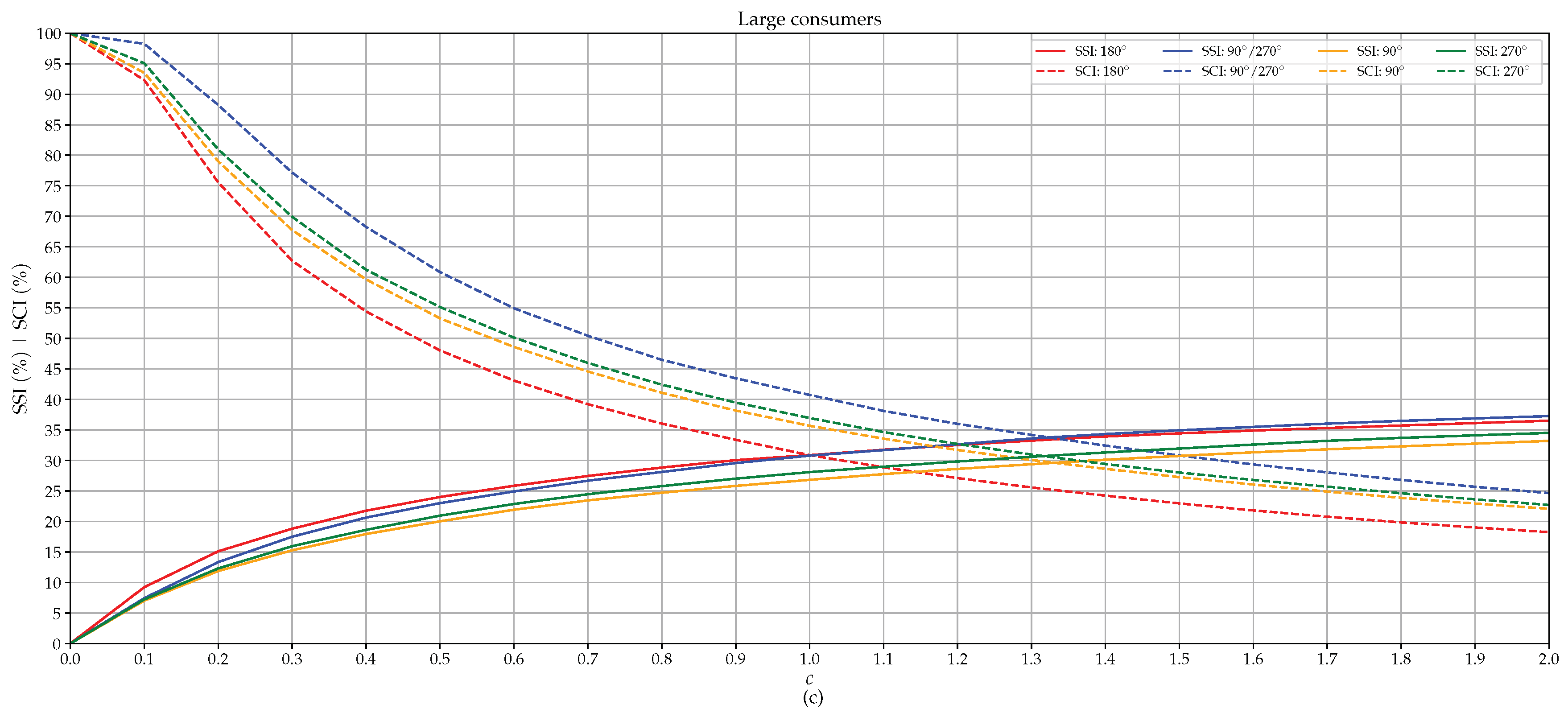
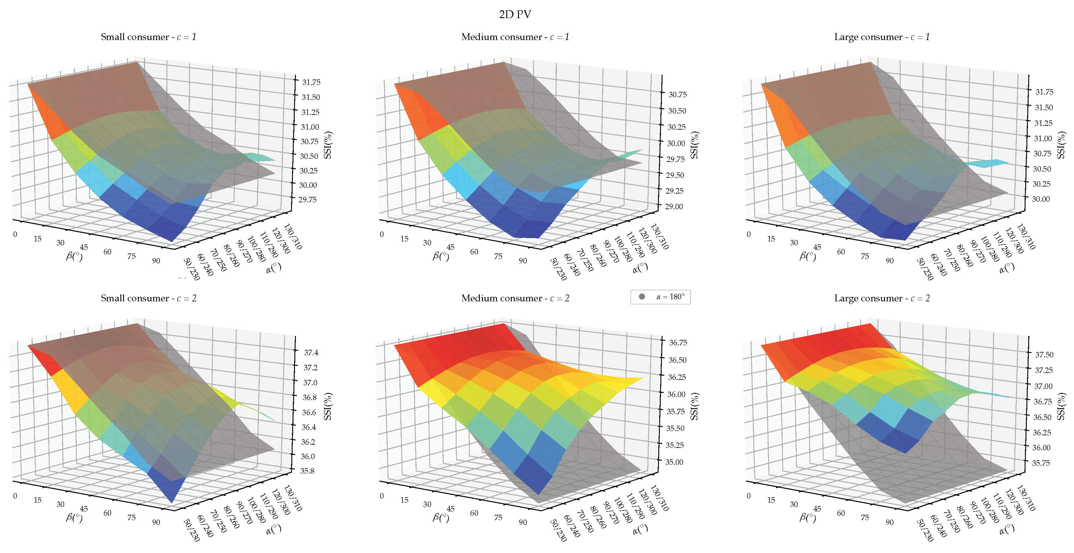
- SCI and SSI: As discussed before, due to evolution of the remuneration mechanisms, SCI is getting more important than the produced PV energy. Furthermore, the higher the SCI, the lower the amount of injected energy to the local grid. In Flanders, injection charges pro rata the injected energy will be applied for residential grid users. With respect to the SSI, it is obvious that end users want to minimize the purchased energy from the grid and thus maximize this value. Both indexes strongly depend on the household’s electricity consumption behaviour. This emphasizes the importance of using real measured load profiles. This analysis will be performed separately for the three different consumption classes in order to detect the particularities for each type of consumer.
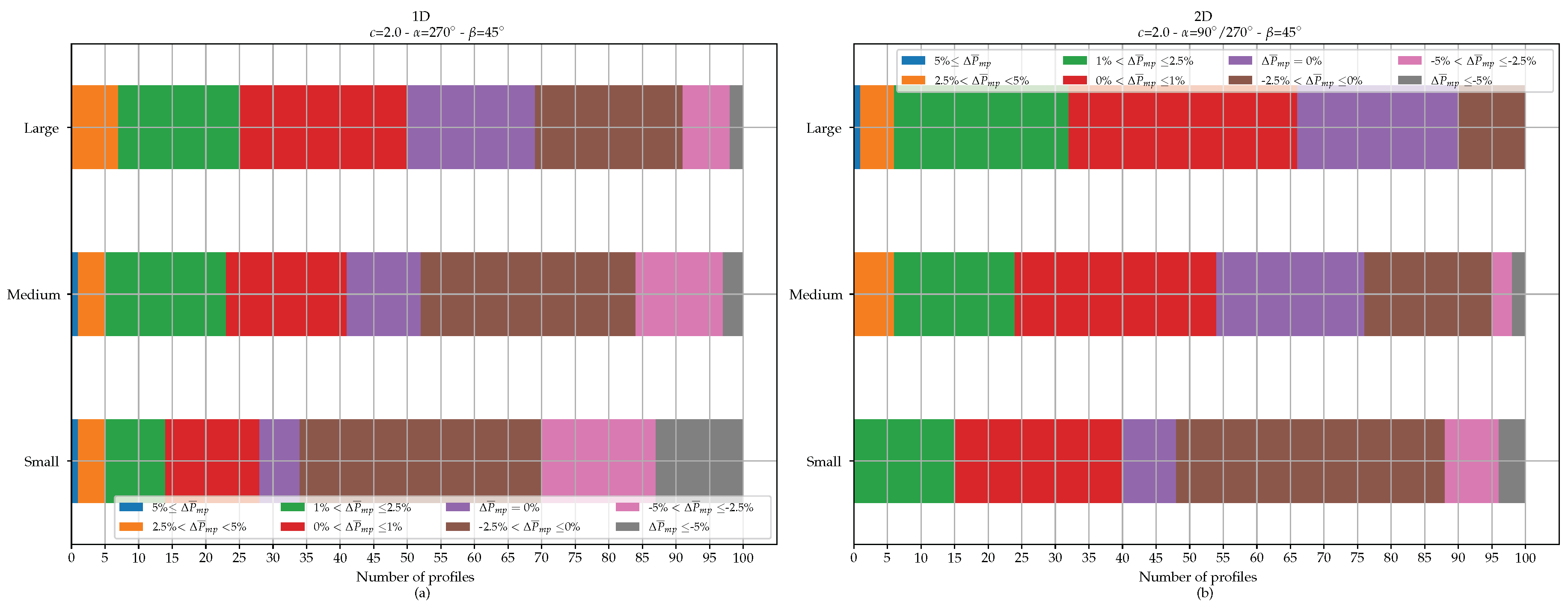
- Peak reduction: The distribution grid tariffs in the electricity bill of residential grid users is today mainly based on the amount of energy taken from the grid. However, a tendency to more capacity-based tariffing is noticeable in many European countries. This evolution is mainly driven by the expected increasing penetration of renewable energy in the distribution grid and the electrification of mobility and heating [27,28]. By introducing capacity-based tariffs, load shifting and other peak reduction measures could be incentivised. Another more viable solution would be to optimize the orientation of the PV panels in order to reduce the morning and/or evening consumption peaks extracted from the grid. An analysis will be performed to quantify the peak reduction for different type of consumers.
- Save in storage capacity: The general aim of integrating storage facilities is to increase SCI and SSI. By orienting the PV panels in an appropriate way, the SCI and the SSI could already be increased without foreseeing any storage facility. This means that, for a certain desired SSI, a smaller storage capacity could be sized when the PV panels are oriented for instance to east/west instead of to the south.
2. Materials and Methods
2.1. In-Plane Irradiance
- -
- Liu & Jordan: This model is the most cited and the simplest isotropic model. This means that it assumes that the diffuse radiation is distributed uniformly over the sky dome. Moreover, it considers the ground reflection to be diffuse [29].
- -
- Klucher: Klucher stated that the isotropic model of Liu & Jordan provides good results for overcast skies but underestimate the radiation for clear and partly overcast skies. To overcome this error, Klucher refined the Temps–Coulson model by taking into account the circumsolar and horizon brightening [23].
- -
- Hay & Davies: The diffuse radiation is here assumed as a combination of an isotropic component and a circumsolar component, without taking into account the horizon brightening. The two compositions of the diffuse radiation are quantified by using an anisotropy index [25].
- -
- Reindl: This model is based on the Hay & Davies model with the addition of diffuse radiation coming from the region near the horizon line. Reindl found that with increasing sky overcast the diffuse radiation increases. Therefore, a modulating factor is included [24].
- -
- Perez: Perez proposed a more detailed analysis of the isotropic diffuse, circumsolar, and horizon brightening radiation. The model takes two sky brightness coefficients into account that are derived empirically [22].
2.2. PV System
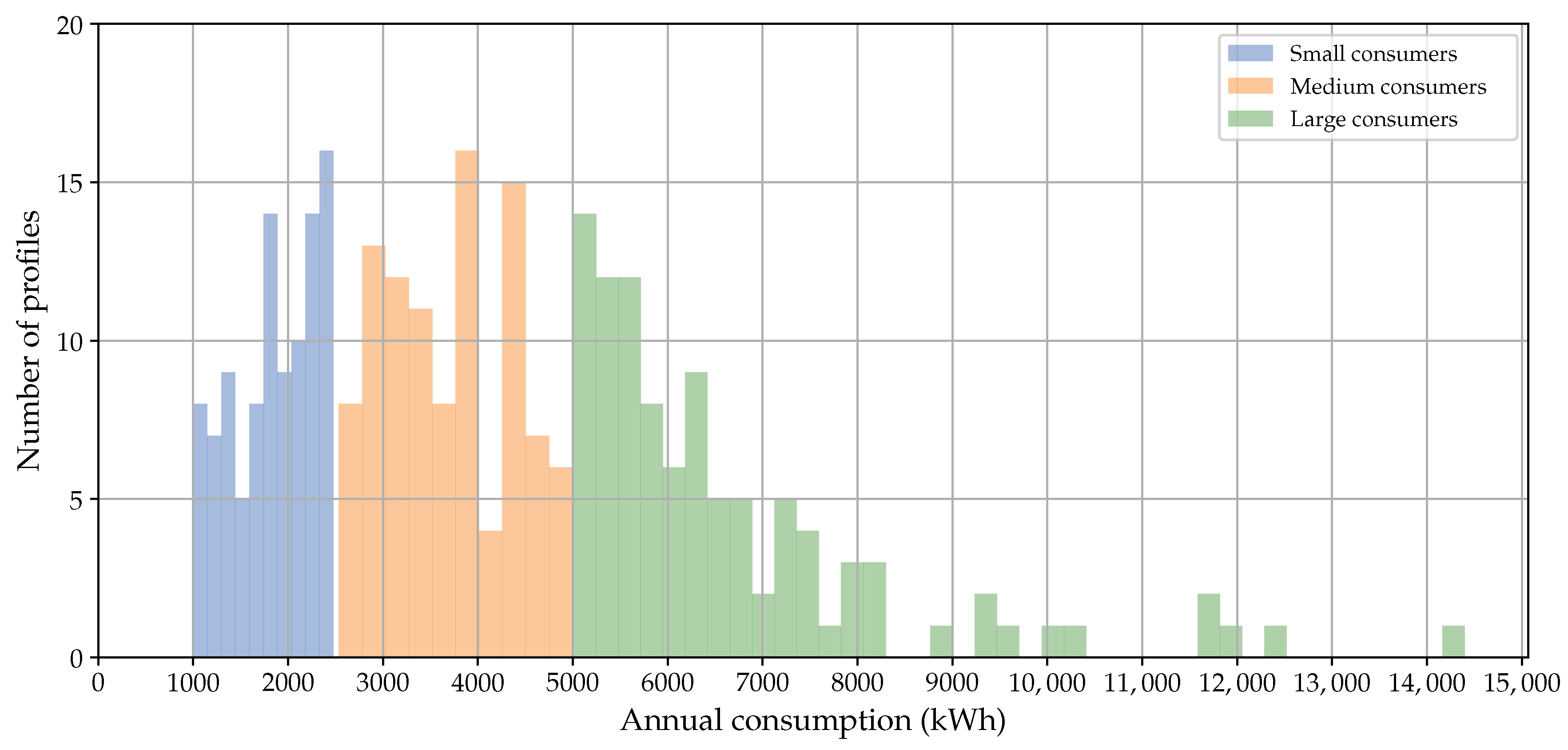
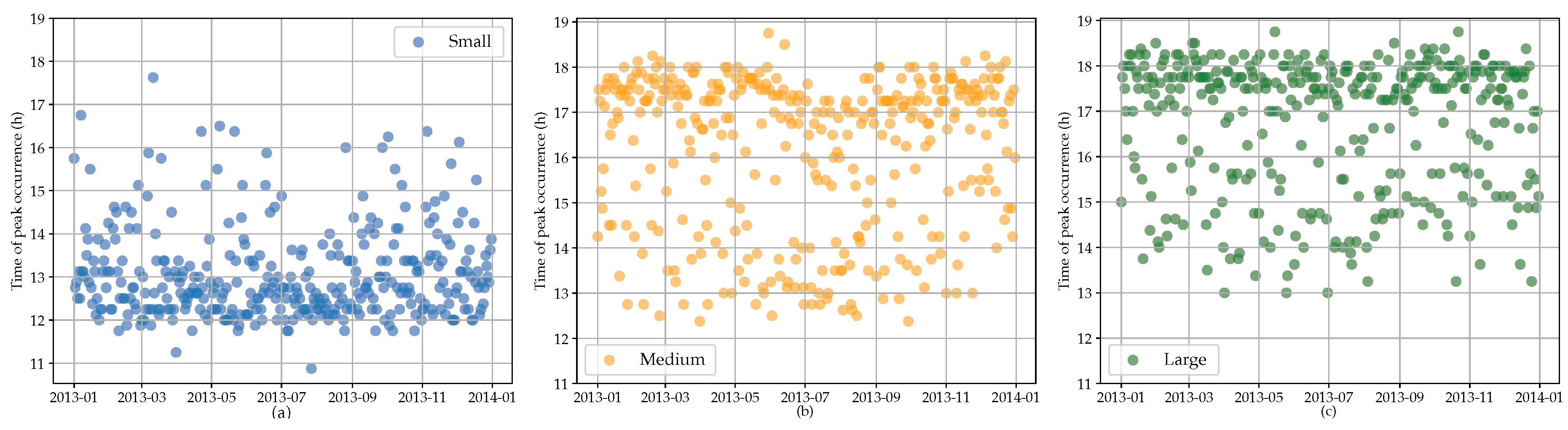
2.3. Consumption Profiles
- -
- Small consumers: consumption between 1000 and 2500 kWh
- -
- Medium consumers: consumption between 2500 and 5000 kWh
- -
- Large consumers: consumption between 5000 and 15,000 kWh
2.4. Measurements
2.5. PV Sizing
2.6. Assessment Criteria
2.7. Practical Aspect
3. Results and Discussion
3.1. SCI and SSI
- -
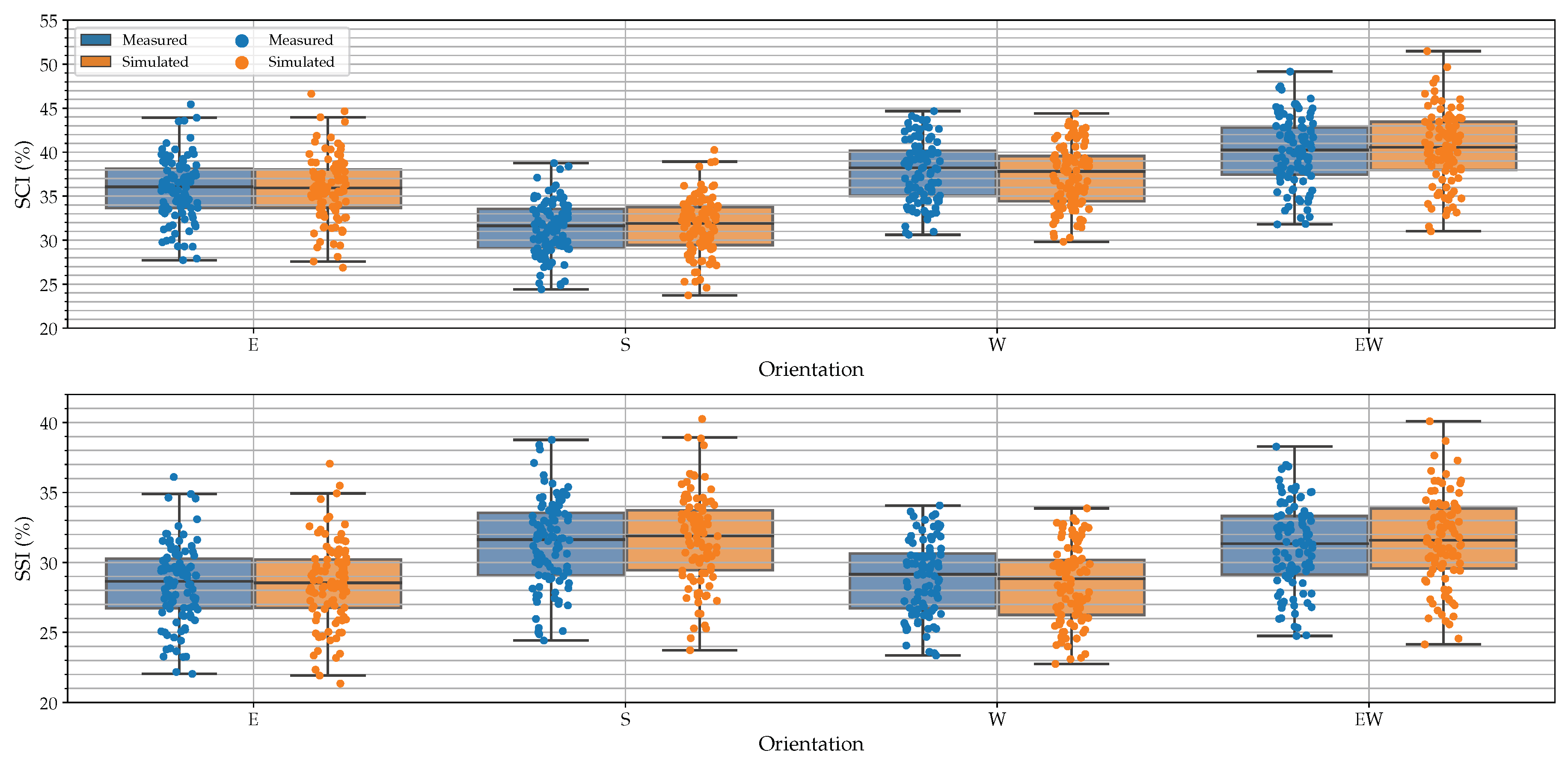
- SCI: increase of 8.62 percent points for the measured PV and 8.66 for the simulated PV
- -
- SSI: decrease of 0.19 percent points for the measured PV and 0.31 for the simulated PV
- -
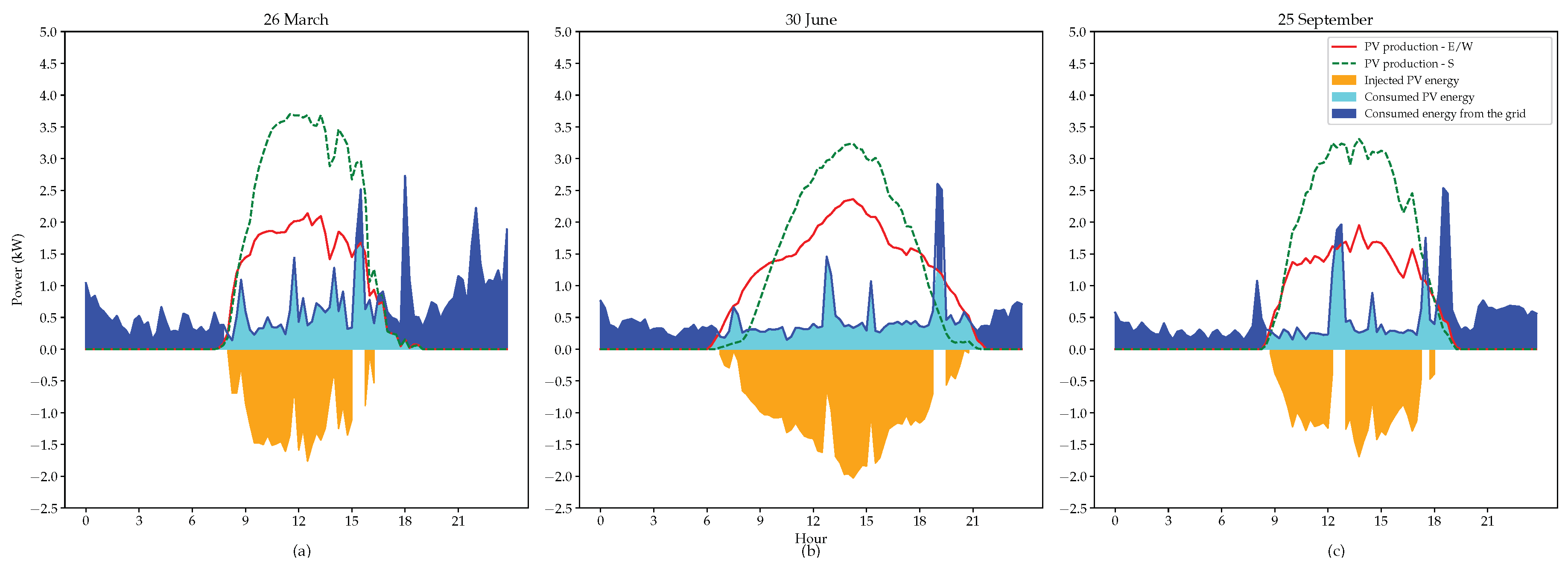
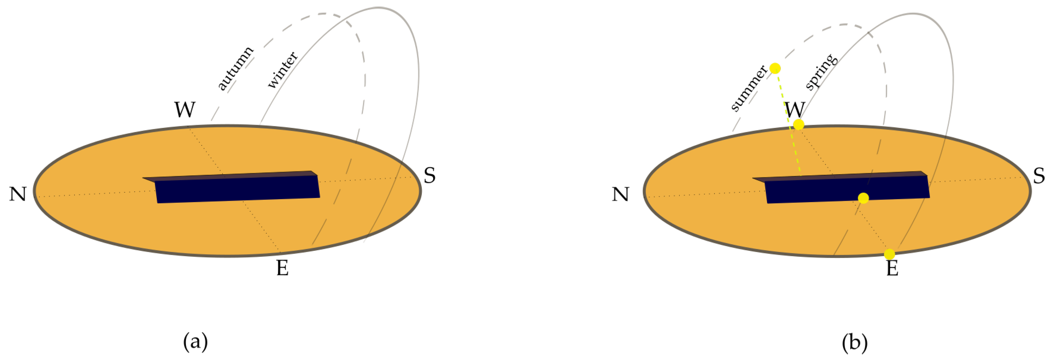
- In the northern hemisphere, the autumn and winter sun rises near the southeast and sets near the southwest. Hence, the direct irradiance is limited, while, during the spring and the summer, the sun rises near the east and northeast and sets near the west and northwest. Consequently, the yield increases during the morning and evening and reaches its maximum when the sun crosses the east and the west. The higher zenith angle of the sun during the spring, and especially during the autumn and the winter, causes the south facing panels to have a more optimal angle of incidence during a larger part of the day. This leads, according to Equation (6), to a higher direct irradiance. Figure 10 illustrates the solar trajectory during different seasons.
- -
- During the winter months, the winter solstice occurs. The earth’s poles are tilted away from the sun causing shorter daylight. Accordingly, during these months, a south-oriented PV installation is more interesting to cover the day consumption.
3.2. Peak Reduction
3.3. Storage
3.4. General Overview
- -
- Due to the non-optimal orientation, the annual yield () for west and east/west-oriented PV is approximately 24% less than for a south-oriented PV installation.
- -
- The maximum produced power is especially lower for an east/west-oriented PV installation. The reduction amounts almost 26.01% while for a west-oriented PV installation it amounts almost 4%. The lower peak power can create two benefits. The lower peak implies that the inverter can be sized smaller. Secondly, a smaller inverter leads to lower grid tariff for prosumers, at least in Flanders (Belgium), where this tariff is dependent on the AC-power of the inverter [48].
- -
- A last point concerns the injected energy. This could also be represented as the complement of the self-consumption. This is almost 6.5% lower for 2D PV and 4.5% for 1D PV. The lower the injected energy, the lower the grid load. Moreover, the new grid tariff structure proposed by the Flemish regulator (VREG) includes a tariff that is calculated pro rata the injected energy.
4. Conclusions
Author Contributions
Funding
Acknowledgments
Conflicts of Interest
References
- European Commission. National Energy and Climate Plans 2020 (NECPs). Available online: https://ec.europa.eu/info/energy-climate-change-environment/overall-targets/national-energy-and-climate-plans-necps_en (accessed on 1 August 2020).
- IEA. Global CO2 Emissions in 2019. Available online: https://www.iea.org/articles/global-co2-emissions-in-2019 (accessed on 1 August 2020).
- Schmela, M. Global Market Outlook For Solar Power: 2019–2023; SolarPower Europe Brussels: Brussels, Belgium, 2018; pp. 8–26. [Google Scholar]
- Kato, T. Record Efficiency for Thin-Film Polycrystalline Solar Cells up to 22.9% Achieved by Cs-Treated Cu(In,Ga)(Se,S)2. IEEE Photovolt. 2019, 9, 325–331. [Google Scholar] [CrossRef]
- Taguchi, M. 24.7% Record Efficiency HIT Solar Cell on Thin Silicon Wafer. IEEE Photovolt. 2014, 10, 96–100. [Google Scholar] [CrossRef]
- IEA. Task1: Strategic PV Analysis and Outreach. In Snapshot of Global PV Markets 2020; Masson, G., Ed.; IEA: Paris, France, 2020; pp. 10–15. [Google Scholar]
- Axaopoulos, P.J. Energy and Economic Comparative Study of a Tracking vs a Fixed Photovoltaic System in the Northern Hemisphere. Nova Energy Environ. Econ. 2013, 21, 1–20. [Google Scholar]
- Hersch, P.; Zweibel, K. Basic Photovoltaic Principles and Methods; Bird, R., Ed.; Technical Information Office: Springfield, CA, USA, 1982; pp. 5–8.
- Jacobson, M.Z.; Jadhav, V. World estimates of PV optimal tilt angles and ratios of sunlight incident upon tilted and tracked PV panels relative to horizontal panels. Sol. Energy 2018, 169, 55–66. [Google Scholar] [CrossRef]
- Soulayman, S. Optimal Tilt Angle and Maximum Possible Solar Energy Gain at High Latitude Zone. Sol. Energy Res. 2016, 12, 25–35. [Google Scholar]
- Wirth, H. Recent Facts about Photovoltaics in Germany; Fraunhofer Institute for Solar Energy Systems ISE: Freiburg, Germany, 2020; Available online: https://www.ise.fraunhofer.de/content/dam/ise/en/documents/publications/studies/recent-facts-about-photovoltaics-in-germany.pdf (accessed on 3 August 2020).
- European Commission. State Aid: Commission Endorses Three French Initiatives to Produce More Than 17 Gigawatts in Renewable Energy. Available online: https://ec.europa.eu/commission/presscorner/detail/en/IP_17_1231 (accessed on 3 August 2020).
- Solar Guide. Smart Export Guarantee to Replace FiT from 2020. Available online: https://www.solarguide.co.uk/smart-export-guarantee-replace-fit#/ (accessed on 3 August 2020).
- Ofgem. Feed-In Tariff (FIT) Rates. Available online: https://www.ofgem.gov.uk/environmental-programmes/fit/fit-tariff-rates (accessed on 3 August 2020).
- VREG. De Digitale Meter bij Zonnepaneleneigenaars. Available online: https://www.vreg.be/nl/de-digitale-meter-bij-zonnepaneleneigenaars (accessed on 3 August 2020).
- VEA. Persbericht: Vlaanderen Blijft Inzetten op Zonne-Energie. Available online: https://www.energiesparen.be/nieuws/persbericht/vlaanderen-blijft-inzetten-op-zonne-energie (accessed on 3 August 2020).
- Van Ryckeghem, J.; Delerue, T.; Bottenberg, A.; Rens, J.; Desmet, J. Decongestion of the distribution grid via optimised location of PV-battery systems. Conf. PQ EMC 2017, 24, 573–577. [Google Scholar] [CrossRef][Green Version]
- Weniger, J.; Tjaden, T.; Quaschning, V. Sizing of residential PV battery systems. Energy Procedia 2014, 46, 78–87. [Google Scholar] [CrossRef]
- Lahnaoui, A.; Stenzel, P.; Linssen, J. Tilt angle and orientation impact on the techno-economic performance of photovoltaic battery systems. Energy Procedia 2017, 105, 4312–4321. [Google Scholar] [CrossRef]
- Mubarak, R.; Luiz, E.W.; Seckmeyer, G. Why PV Modules Should Preferably No Longer Be Oriented to the South in the Near Future. Energies 2019, 12, 4528. [Google Scholar] [CrossRef]
- Laveyne, J.I.; Bolazakov, D.; Van Eetvelde, G.; Vandevelde, L. Impact of Solar Panel Orientation on the Integration of Solar Energy in Low-Voltage Distribution Grids. J. Photoenergy 2020. [Google Scholar] [CrossRef]
- Perez, R.; Ineichen, P.; Seals, R.; Michalsky, J.; Stewart, R. Modeling daylight availability and irradiance components from direct and global irradiance. Sol. Energy 1990, 44, 271–289. [Google Scholar] [CrossRef]
- Klucher, T.M. Evaluation of models to predict insolation on tilted surfaces. Sol. Energy 1990, 23, 111–114. [Google Scholar] [CrossRef]
- Reindl, D.T.; Beckman, W.A.; Duffie, J.A. Evaluation of hourly tilted surface radiation models. Sol. Energy 1990, 45, 9–17. [Google Scholar] [CrossRef]
- Davies, J.A.; Hay, J.E. Calculation of the solar radiation incident on an inclined surface. In Proceedings of the 1st Canadian Solar Radiation Data Workshop, Toronto, ON, Canada, 17–19 April 1978; pp. 59–72. [Google Scholar]
- Eurostat. Energy Statistics-Electricity Prices for Domestic and Industrial Consumers, Price Components. Available online: https://ec.europa.eu/eurostat/cache/metadata/en/nrg_pc_204_esms.htm (accessed on 3 August 2020).
- Consortium of AF-Mercados, REF-E and Indra. Final Report: Study on Tariff Design for Distribution Systems. Available online: https://ec.europa.eu/energy/sites/ener/files/documents/20150313%20Tariff%20report%20fina_revREF-E.PDF (accessed on 3 August 2020).
- VREG. Tariefmethodologie Voor Distributie Elektriciteit en Aardgas Gedurende de Reguleringsperiode 2021–2024. Available online: https://www.vreg.be/sites/default/files/Tariefmethodologie/2021-2024/tariefmethodologie_reguleringsperiode_2021-2024.pdf (accessed on 3 August 2020).
- Liu, B.; Jordan, R. Daily insolation on surfaces tilted towards equator. ASHRAE 1961, 10, 526–541. [Google Scholar]
- Demain, C.; Journée, M.; Bertrand, C. Evaluation of different models to estimate the global solar radiation on inclined surfaces. Renew. Energy 2013, 50, 710–721. [Google Scholar] [CrossRef]
- Maleki, S.A.M.; Hizam, H.; Gomes, C. Estimation of Hourly, Daily and Monthly Global Solar Radiation on Inclined Surfaces: Models Re-Visited. Energies 2017, 10, 134. [Google Scholar] [CrossRef]
- Nikiforiadis, N. Modeling Solar Irradiance; School of Science & Technology: Thesaaloniki, Greece, 2014. [Google Scholar]
- Mubarak, R.; Hofmann, M.; Riechelmann, S.; Seckmeyer, G. Comparison of Modelled and Measured Tilted Solar Irradiance for Photovoltaic Applications. Energies 2017, 11, 1688. [Google Scholar] [CrossRef]
- Spencer, J.W. Fourier series representation of the sun. Search 1971, 2, 172. [Google Scholar]
- Reno, M.J.; Hansen, C.W.; Stein, J.S. Global Horizontal Irradiance Clear Sky Models: Implementation and Analysis; Sandia National Laboratories, U.S. Department of Energy: Oak Ridge, TN, USA, 2007. Available online: https://prod-ng.sandia.gov/techlib-noauth/access-control.cgi/2012/122389.pdf (accessed on 5 August 2020).
- Holm, W.F.; Clifford, W.H.; Mikofski, M.A. pvlib python: A python package for modeling solar energy systems. Open Source Softw. 2018, 3, 884. [Google Scholar]
- King, D.L.; Boyson, W.E.; Kratochvill, J.A. Photovoltaic Array Performance Model; Sandia National Laboratories, U.S. Department of Energy: Oak Ridge, TN, USA, 2004. Available online: https://prod-ng.sandia.gov/techlib-noauth/access-control.cgi/2004/043535.pdf (accessed on 6 August 2020).
- King, D.L.; Gonzalez, S.; Galbraith, G.M.; Boyson, W.E. Performance Model for Grid-Connected Photovoltaic Inverters; Sandia National Laboratories, U.S. Department of Energy: Oak Ridge, TN, USA, 2007. Available online: https://citeseerx.ist.psu.edu/viewdoc/download?doi=10.1.1.464.6452&rep=rep1&type=pdf (accessed on 6 August 2020).
- Mondol, J.D.; Yohanis, Y.G.; Norton, B. The impact of array inclination and orientation on the performance of a grid-connected photovoltaic system. Renew. Energy 2007, 32, 118–140. [Google Scholar] [CrossRef]
- Mondol, J.D.; Yohanis, Y.G.; Norton, B. Optimal sizing of array and inverter for grid-connected photovoltaic systems. Sol. Energy 2006, 80, 1517–1539. [Google Scholar] [CrossRef]
- PVOutput Dataset. Available online: https://pvoutput.org/ (accessed on 15 January 2019).
- Beck, T.; Kondziella, H.; Huard, G.; Bruckner, T. Assessing the influence of the temporal resolution of electrical load and PV generation profiles on self-consumption and sizing of PV-battery systems. Appl. Energy 2016, 173, 331–342. [Google Scholar] [CrossRef]
- Ried, S.; Jochem, P.; Fichtner, W. Profitability of Photovoltaic Battery Systems Considering Temporal Resolution. In Proceedings of the 2015 12th International Conference on the European Energy Market (EEM), Lisbon, Portugal, 19–22 May 2015. [Google Scholar]
- Bertrand, C.; Housmans, C.; Leloux, J. Solar Irradiation from the Energy Production of Residential PV Systems (Spider); RMI: Brussels, Belgium, 2017; Available online: https://www.belspo.be/belspo/brain-be/projects/FinalReports/SPIDER_FinRep.pdf (accessed on 1 August 2020).
- Wyatt, P. A dwelling-level investigation into the physical and socio-economicdrivers of domestic energy consumption in England. Energy Policy 2013, 60, 540–549. [Google Scholar] [CrossRef]
- Anderson, B.; Torriti, J. Explaining shifts in UK electricity demand using time use data from 1974 to 2014. Energy Policy 2018, 123, 544–557. [Google Scholar] [CrossRef]
- Sarasketa-Zabala, E.; Martinez-Laserna, E.; Berecibar, M.; Gandiaga, I.; Rodriguez-Martinez, L.M.; Villarreal, I. Realistic lifetime prediction approach for Li-ion batteries. Appl. Energy 2016, 162, 839–852. [Google Scholar] [CrossRef]
- VREG. Prosumententarief 2020. Available online: https://www.vreg.be/nl/prosumententarief-2020 (accessed on 13 August 2020).
- Jones, K.B.; Benett, E.C.; Ji, F.W.; Kazerooni, B. Beyond Community Solar: Aggregating Local Distributed Resources for Resilience and Sustainability. In How Distributed Energy Resources are Disrupting the Utility Business Model; Sioshansi, F.P., Ed.; Menlo Energy Economics: Walnut Creek, CA, USA, 2017; pp. 65–81. [Google Scholar]
- Noll, D.; Dawes, C.; Varun, R. Solar Community Organizations and active peer effects in the adoption of residential PV. Energy Policy 2014, 67, 330–343. [Google Scholar] [CrossRef]


| Parameter | Module |
|---|---|
| Type | Sunpower SPR-230-WHT-U |
| Technology | Mono-Si |
| Peak Power | 230 W |
| Installation | A | B | C |
|---|---|---|---|
| 90° | 180° | 270° | |
| 45° | 45° | 45° | |
| 7590 W | 5750 W | 5060 W | |
| PV technology | Poly-si | Poly-si | Poly-si |
| Module type | Atersa A-230P | BS-250P | Mage Solar 230/6PJ |
| 6300 W | 215 W | 5060 W | |
| Inverter type | SMA SMC6000A | Enphase M215 | SMA SB 5000TL-20 |
| Installation (Orientation) | A (E) | B (S) | |||||
| Percentile | q25 | q50 | q75 | q25 | q50 | q75 | |
| SCI (%) | Measured | 33.64 | 36.06 | 38.11 | 29.07 | 31.63 | 33.55 |
| Simulated | 33.67 | 35.93 | 38.03 | 29.44 | 31.89 | 33.74 | |
| SSI (%) | Measured | 26.73 | 28.65 | 30.28 | 29.07 | 31.63 | 33.55 |
| Simulated | 26.75 | 28.54 | 30.22 | 29.44 | 31.89 | 33.74 | |
| Installation (Orientation) | C (W) | A+C (E/W) | |||||
| Percentile | q25 | q50 | q75 | q25 | q50 | q75 | |
| SCI (%) | Measured | 35.04 | 38.22 | 40.18 | 37.43 | 40.25 | 42.79 |
| Simulated | 34.41 | 37.82 | 39.57 | 37.99 | 40.55 | 43.46 | |
| SSI (%) | Measured | 26.73 | 29.15 | 30.65 | 29.14 | 31.34 | 33.32 |
| Simulated | 26.25 | 28.84 | 30.18 | 29.58 | 31.58 | 33.84 | |
| SSI (%) | c | 0.5 | 1 | 1.5 | 2 |
|---|---|---|---|---|---|
| Small consumers | S | 23.91 | 30.77 | 34.62 | 36.86 |
| E/W | 23.13 | 30.63 | 34.61 | 37.11 | |
| [points] | −0.78 | −0.14 | −0.01 | 0.25 | |
| Medium consumers | S | 23.55 | 30.25 | 33.64 | 35.77 |
| E/W | 22.81 | 29.92 | 33.80 | 36.36 | |
| [points] | −0.75 | −0.33 | 0.16 | 0.59 | |
| Large consumers | S | 24.01 | 30.87 | 34.43 | 36.50 |
| E/W | 23.00 | 30.79 | 34.93 | 37.26 | |
| [points] | −1.01 | −0.07 | 0.50 | 0.76 |
| SSI (%) | ||||||||
|---|---|---|---|---|---|---|---|---|
| c | 1 | 2 | ||||||
| 90° | 270° | 90°/270° | 180° | 90° | 270° | 90°/270° | 180° | |
| 0° | 31.94 | 31.94 | 31.94 | 31.94 | 37.71 | 37.71 | 37.71 | 37.71 |
| 15° | 29.74 | 30.56 | 31.17 | 31.73 | 35.85 | 36.69 | 37.46 | 37.40 |
| 30° | 27.98 | 29.08 | 30.90 | 31.28 | 34.30 | 35.73 | 37.36 | 36.93 |
| 45° | 26.82 | 28.09 | 30.79 | 30.87 | 33.20 | 34.51 | 37.26 | 36.50 |
| 60° | 26.19 | 27.47 | 30.64 | 30.50 | 32.69 | 33.94 | 37.16 | 36.08 |
| 75° | 25.97 | 27.28 | 30.50 | 30.20 | 32.38 | 33.80 | 37.03 | 35.73 |
| 90° | 26.33 | 27.55 | 30.63 | 30.07 | 32.51 | 34.03 | 36.98 | 35.60 |
| (Percent Points) | 1D | 2D |
|---|---|---|
| 270° | 90°/270° | |
| −23.98 | −24.41 | |
| SSI | −1.72 | 0.94 |
| SCI | 4.59 | 6.46 |
| −0.06 | −0.39 | |
| −4.84 | −26.01 | |
| - | −6.16 |
© 2020 by the authors. Licensee MDPI, Basel, Switzerland. This article is an open access article distributed under the terms and conditions of the Creative Commons Attribution (CC BY) license (http://creativecommons.org/licenses/by/4.0/).
Share and Cite
Azaioud, H.; Desmet, J.; Vandevelde, L. Benefit Evaluation of PV Orientation for Individual Residential Consumers. Energies 2020, 13, 5122. https://doi.org/10.3390/en13195122
Azaioud H, Desmet J, Vandevelde L. Benefit Evaluation of PV Orientation for Individual Residential Consumers. Energies. 2020; 13(19):5122. https://doi.org/10.3390/en13195122
Chicago/Turabian StyleAzaioud, Hakim, Jan Desmet, and Lieven Vandevelde. 2020. "Benefit Evaluation of PV Orientation for Individual Residential Consumers" Energies 13, no. 19: 5122. https://doi.org/10.3390/en13195122
APA StyleAzaioud, H., Desmet, J., & Vandevelde, L. (2020). Benefit Evaluation of PV Orientation for Individual Residential Consumers. Energies, 13(19), 5122. https://doi.org/10.3390/en13195122