Evaluation of Wind Flow Characteristics by RANS-Based Numerical Site Calibration (NSC) Method with Met-Tower Measurements and Its Application to a Complex Terrain

Abstract

The performance of wind turbines is not only dependent on the wind turbine design itself, but is also dependent on the accurate assessment of wind resources at the installation site. In this paper, the numerical site calibration (NSC) method using three-dimensional Reynolds-averaged Navier–Stokes (RANS) simulation was proposed to accurately forecast the wind flow characteristics of wind turbine sites with complex terrains, namely Methil in Scotland, and Haenam in South Korea. From NSC at the Methil and Haenam sites, it was shown that the complicated and vortical flow fields around hills and valleys were captured using the three-dimensional RANS CFD simulation in Ansys CFX software based on a high-resolution scheme with a renormalization group (RNG)-based k-ε turbulence model. It was also shown that topographically induced wind profile and turbulence intensity over a local-scale complex terrain are remarkably dominated by flow separation after passing hills. It was concluded that the proposed NSC method using three-dimensional RANS simulation with a high-resolution scheme was an economically useful method for evaluating wind flow characteristics numerically to assess wind turbine sites with complex terrains and designing the wind farm layout.

1. Introduction

Wind energy has been in the spotlight as a major source of renewable energy, and its levelized cost of energy (LCOE) has reduced a lot to become a favorable alternative source to fossil fuel energy. With innovatively engineered design of blade airfoils and planform using increased computational performance, wind turbines have been designed to extract wind energy as close as possible to the Betz limit of 59.3% [1].

Since onshore wind turbines are installed not only in flat areas as preferred sites, but also in areas surrounded by hills or valleys, it is important to understand the geological effect on wind flow approaching the wind turbine to maximize the annual energy production (AEP). Therefore, in order to accurately evaluate the performance of a wind turbine overall, it is essential to forecast the wind flow characteristics such as velocity profile and turbulence intensity related to the wind turbine installation site. Furthermore, it is recommended to choose a wind turbine of a design grade adequate for the estimated wind conditions in order to maximize durability and economic benefits [2,3,4].

There are many studies investigating the effect of wake on wind speed and the performance of a single wind turbine or multiple wind turbines like on a wind farm. Ainslie outlined the features of wind turbine wakes and described a numerical model to calculate the wake flow field [5]. Vermeer et al. studied the aerodynamics of horizontal axis wind turbine wake and reviewed both the near and the far wake regions. For the far wake, both a single turbine and wind farm effects were experimentally and numerically studied to understand how the far wake decays downstream [6]. Sanderse et al. also reviewed numerical calculations of wind turbine wake aerodynamics with different computational fluid dynamics (CFD) techniques for modeling the rotor and the wake [7]. Several works were focused on the validation of wake simulation models with measurements from wind tunnel experiments and directly from wind farms. Chamorro and Porte-Agel performed wind tunnel experiments to study turbulence in the wake of a wind turbine model [8], and Schumann et al. investigated wind turbine wakes in a wind tunnel with two similar models of wind turbine [9]. Gaumond et al. used power production data from the Horns Rev and Lillgrund offshore wind farms to compare three engineering wake models [10]. In addition, Barthelmie et al. evaluated the commonly used wake models for predicting wind speed decrease downstream of a wind turbine based on six experiments using a ship-mounted sodar at a small wind farm [11]. Specifically, Barthelmie et al. used integrated Doppler lidar data from the Perdigao experiment to measure wind turbine wakes and also to characterize wind gusts in a complex terrain [12,13]. Energy extraction out of various wind farm layouts was investigated with a wake effect model [14], and it showed at most a 30% decrease in the extracted energy depending on the wind farm layouts. Jadhav and Roy [15] examined the impact of wind turbine wake on the economic dispatch of a power system and stated that the wake effect significantly influenced the overall cost of operation and the loss of transmission. Wind turbine loads under the wake effect were studied based on the measurements obtained from Vindeby offshore wind farm in Denmark [16], which showed that the turbulence intensity and fatigue loading in the wind turbine can increase by 5–15% according to the layout of wind farm. Kim et al. [17] also investigated the wake effect from the wind farm layout and showed a 7% reduction in AEP and a 30–50% increment in damage equivalent load (DEL).

In addition, there are many interesting works related to noise caused by a complex terrain. A major obstacle to the diffusion and worldwide spread of wind energy is represented by its produced noise [18,19]. Wind turbine do not emit high levels of noise, but they are much more annoying than other common noise sources [20,21]. Especially in hilly areas, quietness is required and even lower noises are perceived much more. Prevention and monitoring play key roles in avoiding well-known health related issues such as sleep disorders [22], learning impairment [23,24], hypertension ischemic heart disease [25], and annoyance [26]. In this regard, a proper knowledge of winds will also be useful to better predict the noise emission of a wind farm through detailed procedures [27].

According to the International Electrotechnical Commission (IEC) 61400-12-1 [28], site calibration procedures must be followed before installing wind turbines except for regions that show only minor variations in topography. For a site calibration, anemometers are installed at the prospective wind turbine site and a reference site nearby, and the correlation of the wind conditions at the two sites would be derived based on the data acquired during a specific period. The correlation is then used to forecast the wind characteristics at the prospective installation site. For this correlation process, two meteorological towers have to be erected to measure the speed and the direction of the wind, requiring significant amounts of time and cost. Moreover, the site calibration is suitable for a relatively flat topography with stable winds, and therefore it is difficult to obtain accurate forecasts in topographically complicated regions such as Korea, which has a lot of mountainous terrains resulting in unstable winds.

According to Annex B of the IEC 61400-12 standard, the site calibration is required except for cases where the maximum slope value and the maximum terrain variation from the plane at the prospective installation site are smaller than the recommended specific values. The standard suggests that a flow model can be used to determine whether a site calibration measurement can be avoided or not if the terrain characteristics are within an additional 50% of the limits of maximum slope value. In that case, if the difference in wind speed between the anemometer and the installation site is within 1% at 10 m/s, then the site calibration measurement is not necessary.

Sanada et al. [29] conducted studies on forecasting unstable winds at complex terrains using a numerical site calibration method (NSC) based on flow models from computational fluid dynamics (CFD) [30,31]. The cross-validation of the numerical simulations with a high-resolution scheme and k–ε model against wind tunnel experimental results and on-site measurements indicates a good agreement [32].

In this paper, the numerical site calibration method (NSC) employing three-dimensional Reynolds-averaged Navier–Stokes (RANS) approach was proposed to numerically forecast the wind flow characteristics at the wind turbine installation sites without the installation of expensive meteorological towers for the type certification of a single wind turbine. Two specific areas, Methil in Scotland and Haenam located to the west of South Korea, were first investigated with the given topography data and a three-dimensional RANS CFD simulation solver in Ansys CFX [33].

2. Numerical Analysis Method

2.1. Numerical Site Calibration (NSC) Method

The numerical site calibration method (NSC) is a three-dimensional flow analysis method based on computational fluid dynamics (CFD) to forecast the wind condition, and it utilizes the correlation of wind characteristics between the reference sites and the prospective wind turbine installation sites. Compared to traditional site calibration, NSC eliminates the cost of erecting a meteorological tower and can be applied to complex terrains, providing wind resource to accurately estimate the performance of large wind turbines as shown in Figure 1 [34].

In order to establish the evaluation method based on NSC, it is important to clarify the range of application for calculation results and its reliability. Other points which should be also addressed include the characteristics of the numerical analysis code, calculation regions and boundary conditions, and securing statistical significance. Since calculation regions and boundary conditions are important factors for simulating wind conditions, wind condition comparison between measurement data and simulation values must be performed. The comparison needs to show the correlation error between measured and simulated values within 3% to establish the simulation procedure.

2.2. Governing Equation and Turbulence Flow Model

There are three major numerical techniques for modeling turbulent flow fields: direct numerical simulation (DNS), large eddy simulation (LES), and Reynolds-averaged Navier–Stokes (RANS). DNS and LES require substantial calculation resources to analyze a vortex, and it is difficult to apply them to practical engineering problems. With recent developments in computer capacity and capability, there have been a number of studies on the specific behavior of a vortex by performing numerical analyses that apply LES on complex terrains [35,36,37]. On the other hand, RANS uses time-based, ensemble-averaged Navier–Stokes equations and models all of the effects from turbulence. Although RANS yields a lower resolution of analysis than DNS or LES, it is widely used in engineering applications due to the practical aspect of not requiring high-resolution calculation grids [38,39,40,41].

Unlike the complex flow fields inside and outside a wind turbine, in most cases of wind condition analysis, it is difficult to form rapid adverse pressure gradients in the flow direction. Therefore, the k–ε turbulence model, which accurately analyzes turbulence behavior in free-stream regions with small pressure gradients, is chosen preferably for RANS numerical analysis than the Wilcox k–ω turbulence model [42], which provides accurate forecasts of boundary layer separation having the adverse pressure gradients in viscous sub-layer regions. The k–ε turbulence model is widely used by researchers for topography analysis [43]. In particular, the renormalization group (RNG)-based k–ε turbulence model yields forecasts with high reliability in analyzing complex terrains [44]. For this reason, the RNG-based k–ε turbulence model was used for this paper. Even though wall grid-scale is not enough near the surface, the current numerical analysis was also tested using the shear stress transport (SST) turbulence model, which is based on the k–ω turbulence model in order to evaluate the sensitivity of the turbulence model [45]. In this paper, the k–ε turbulence model has been used though two approaches resulted in little difference. The convergence of numerical analysis was determined based on the regular wind speed history at the meteorological tower site.

In the RANS equation, the flow is considered as the ideal gas equation of state. For 3D steady flow simulation, the instantaneous equations of mass, momentum and energy conservation in tensor form can be written as follows [45]. The continuity, momentum and energy equations are given by

$$\frac{\partial \mathsf{\rho }{u}_j}{\partial x_j}=0,$$

(1)

$$\frac{\partial \mathsf{\rho }{u}_i{u}_j}{\partial x_j}=-\frac{\partial \mathrm{p}}{\partial x_i}+\frac{\partial {\mathsf{\tau }}_{ij}}{\partial x_j},$$

(2)

$$\frac{\partial }{\partial x_j}\mathsf{\rho }{u}_j\mathrm{e}=\frac{\partial }{\partial x_j}\left[u_j{\mathsf{\tau }}_{ij}+\frac{C_p\mu }{\mathrm{Pr}}\frac{\partial T}{\partial x_j}-u_j\mathrm{p}\right],$$

(3)

In Equations (1)–(3), $\mathsf{\rho }$ is the air density, $u_j$ is the jth velocity component, ${\mathsf{\tau }}_{ij}$ is the Reynolds stress tensor of eddy viscosity model, p is the air static pressure, e is the air energy, $C_p$ is the specific heat, $\mu$ is the air viscosity, Pr is the Prandtl number, and T is the air temperature. The air viscosity and Prandtl number are given by

$$\mu ={\mu }_l+{\mu }_t,$$

(4)

$$\frac{\mu }{\mathrm{Pr}}=\frac{{\mu }_l}{P{r}_l}+\frac{{\mu }_t}{P{r}_t},$$

(5)

where ${\mu }_l$ is the laminar viscosity, ${\mu }_t$ is the turbulent viscosity calculated by a turbulence model, $P{r}_l$ is the laminar Prandtl number, and $P{r}_t$ is the turbulent Prandtl number. Version 15.0 of Ansys CFX was used in this simulation.

3. Site Information and Boundary Conditions for Numerical Analysis

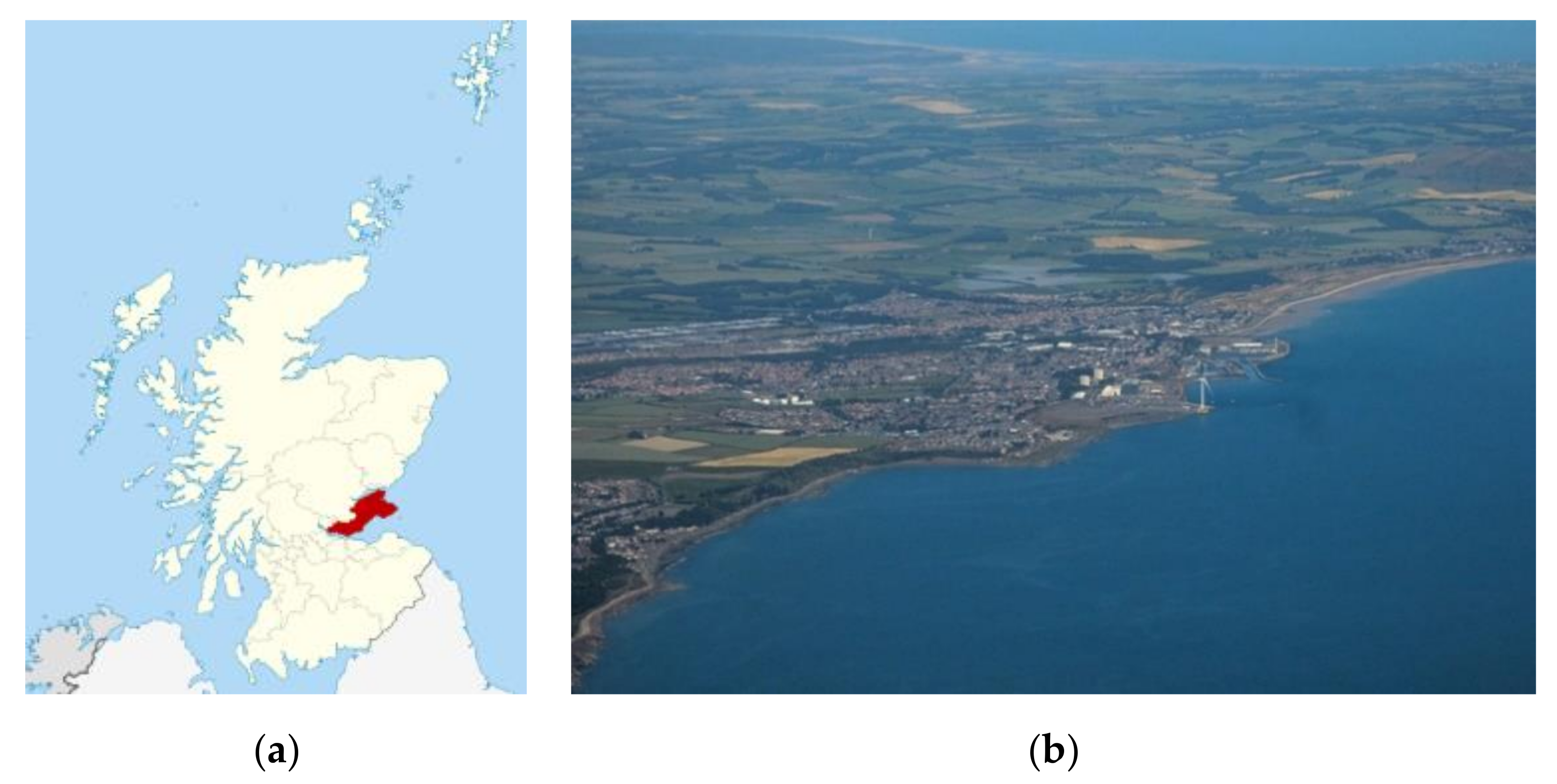
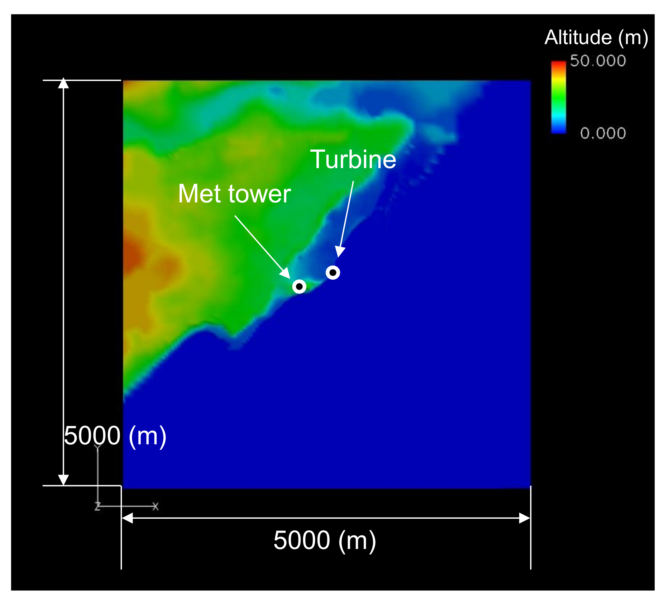
3.1. Wind Turbine Sites

In this paper, two specific sites, Methil in Scotland, and Haenam in South Korea, were selected to evaluate the wind flow characteristics using the proposed NCS method based on RANS simulation as shown in Figure 2 and Figure 3. In both cases, WAsP software was used to transform the Google map into digitalized information for CFD simulation. The Methil site is a sort of flat area with a few steep hills and residential areas, while the Haenam site is quite a complex terrain consisting of many hills and valleys, which is a common characteristic in South Korea.

The velocity at the Met tower at a height of 80 m was measured for six months and

Table 1. Measured velocity data at Methil, Scotland.

Wind Direction (deg)	Velocity at Met Tower (m/s)
120	9.82771
150	9.92642
210	10.2062
300	9.62557
360	10.1512

shows 10 min average velocities at specific wind directions, where the main wind direction was 210 deg.

3.2. Boundary Conditions

To perform numerical site calibration properly, calculation regions and boundary conditions should be defined. Figure 4 shows the calculation regions for this analysis which were set at 5.0 km with a minimum grid interval of 5 m in all directions.

In order to minimize the blockage effect on the analytical results, a sufficient distance of 5 km was maintained from the ground in the vertical direction. As per the boundary conditions, a no-slip condition was applied on the ground surface in the vertical direction, and the roughness length of the sea, land, and residential area were set at 0.0002, 0.03, and 0.4 m, respectively, as written in IEC 61400 part 12 ANNEX A [28]. In addition, a free-slip condition was applied to the ceiling of the calculation region. The wind shear profile of Equation (6) was applied as both entry and exit boundary conditions in the east-west-north-south directions.

$$V\left(H\right)=V\left(H_{hub}\right)\times {\left(\frac{H}{H_{hub}}\right)}^{\alpha },$$

(6)

In Equation (6), V and H denote wind speed and vertical height, respectively, and the subscript hub means the position of the wind turbine hub. α is a heuristic constant that varies according to the atmospheric conditions. In this study, α = 0.2 was used based on the IEC standard. In this work, a turbine with 171 m rotor diameter and 110 m hub height was used.

Table 2. Boundary conditions.

Turbulence Model	RNG k–ε
Numerical scheme	High resolution
Inlet and side boundary conditions	Wind shear profile V(z) = Vhub(Z/Zhub)0.2 (Yaw error = 0 (deg))
Turbulent intensity on inlet region	5%
Outlet boundary condition	Pressure of 10,1300 (Pa)
Terrain boundary condition	No slip with each roughness value
Ceiling boundary condition	Free slip

lists the summary of the boundary conditions for numerical site calibration at the Methil site.

Here, k and ε are computed by the turbulence transportation equation, and the outlet condition was computed through the pressure boundary. Since the Mach number is very low, incompressibility can be assumed, therefore temperature fluctuation is ignorable. The reason for using the RNG k–ε model is that it is difficult to simulate the first cell with a very small height, but it has more freedom in selecting the y + parameter. The simulation convergence was good enough since rms pressure was converged below 10⁻⁶.

3.3. Grid Sensitivity Study

It is necessary to understand the characteristics of the flow analysis code to evaluate the reliability of the calculation outcome. In this study, the effects of grid densities in the horizontal and vertical directions and the turbulence model on the calculation results were evaluated.

Table 3. Grid systems and analysis cases.

No.	Minimum Grid Size in Each Direction	Number of Cells	Domain Size (km)
1	5 m	230 × 230 × 160	5.0 × 5.0 × 5.0
2	10 m	170 × 170 × 120	5.0 × 5.0 × 5.0
3	15 m	115 × 115 × 80	5.0 × 5.0 × 5.0

summarizes the number of cells throughout the calculation region. The grid density distributions in the horizontal direction of grid system numbers 1 and 2 in Table 3 are shown in Figure 5, which indicates that grids were formed around the wind turbine and the meteorological tower. For the current mesh generation, the fully hexahedral mesh was used.

4. Numerical Results

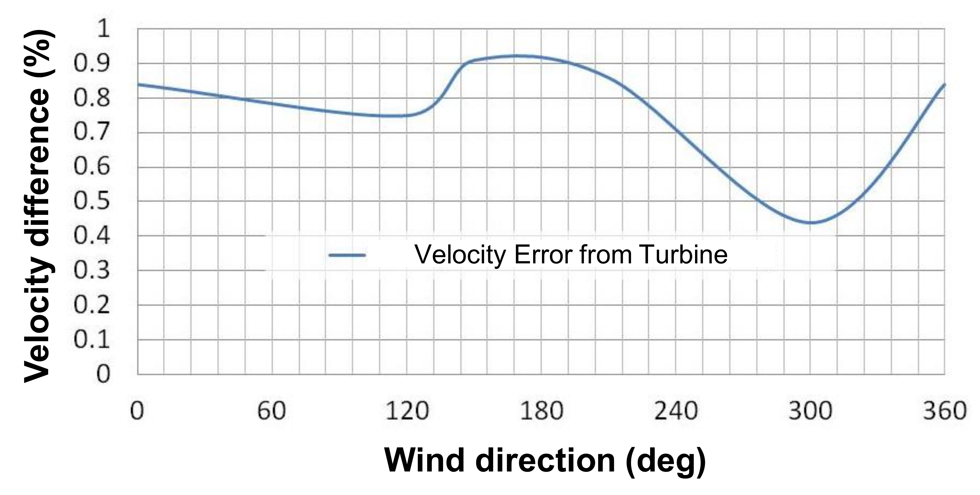
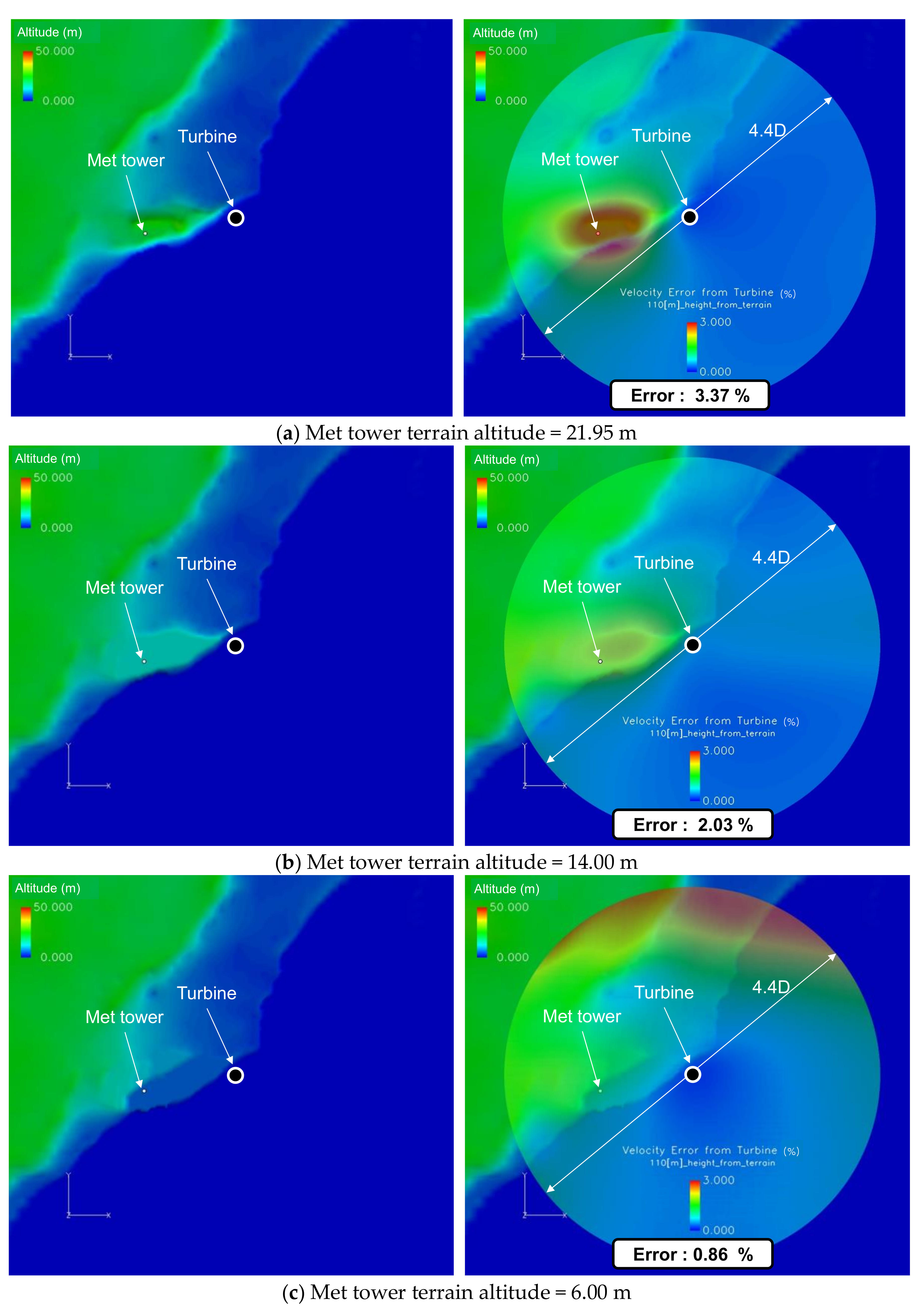
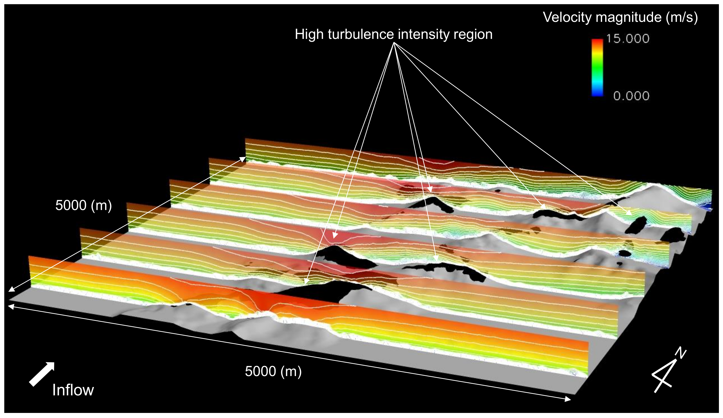
4.1. Methil, Scotland

The digitalized raw image was pre-processed by ICEM to generate grid meshes, then analyzed by Ansys CFX. The numerical results were post-processed using Fieldview software for the high-resolution image as shown in Figure 6.

As expected, the overall topography shows little variation in terms of elevation with only scattered hills. Based on the topography data, the maximum slope value and the maximum terrain variation from the plane were calculated according to the IEC standard part 12 [28]. The calculation results exceeded the specified values due to the high hill on the planned location of the meteorological tower, then it was required to follow the site calibration procedure by installing an additional Met tower at the wind turbine installation location. The numerical analysis based on the 3D RANS simulation was performed to find out the resolution to avoid the required site calibration process.

From the numerical analysis, the effect of the height of the hill on the wind speed difference between the tower location (reference site) and the prospective wind turbine installation site was investigated. The difference in wind speed between the reference site and the prospective wind turbine installation site in the identical wind direction of 210 deg at a boundary wind speed condition of 10.2062 m/s is summarized in

Table 4. Numerical uncertainty results of grid size dependency on wind speed.

Minimum Grid Size (m)	Calculated Velocity at Turbine (m/s)	Measured Velocity at Met Tower (m/s)	Difference (%)
5	9.8623	10.2062	3.37
10	9.8684	10.2062	3.31
15	9.8755	10.2062	3.24

. As listed in Table 4, the effect of grid density on the calculation result is just 0.13%, which is ignorable.

Furthermore, in order to quantitatively evaluate the effect of the turbulence model on the calculation result during RANS simulation, sensitivity analysis was performed on the k–ε turbulence model and the shear stress transport (SST) turbulence model, which has the characteristics of the k–ω turbulence model.

Table 5. Numerical uncertainty results of turbulence model dependency on wind velocity.

Turbulence Model	Calculated Velocity at Turbine (m/s)	Measured Velocity at Met Tower (m/s)	Difference (%)
k–ε	9.8623	10.2062	3.37
SST	9.8571	10.2062	3.42

indicates that the effect of the turbulence model on calculation result is very minimal at 0.05%. Therefore, it could be stated that the uncertainties associated with the effects of grid density and the turbulence model on the calculation outcome are very little.

Figure 7 displays the analytical results according to the variations in the height of the hill when the wind blows in the main direction of 210 deg at 10 m/s. The difference in wind speed between the prospective wind turbine installation site and the surrounding area within a 753 m radius (4.4 × rotor diameter) at the hub height with respect to the wind turbine, as well as the surrounding elevations are shown.

Table 6. Wind speed difference between Met tower and turbine according to the hill height.

Height of Hill (m) (Wind Direction = 210 deg)	Wind Speed Difference (%)
21.95 (original height)	3.37
14.00	2.03
6.00	0.86

shows results of the difference in wind speed between the two sites according to the decrease in the height of the hill where the meteorological tower is to be installed. If the height of the hill decreases to 6 m, the difference in wind speed converges to within 1%, which can potentially eliminate the need for site calibration measurement.

Table 7. Wind speed difference between Met tower and turbine site according to the valid sectors.

Wind Direction (deg)	Velocity at Turbine (m/s)	Velocity at Met Tower (m/s)	Difference (%)
120	9.75387	9.82771	0.75
150	9.83648	9.92642	0.91
210 (main direction)	10.1186	10.2062	0.85
300	9.58328	9.62557	0.44
360	10.0659	10.1512	0.84

and Figure 8 also show that the difference in wind speed is within 1% across the valid measurement sectors if the hill height is adjusted to 6 m, which confirms that site calibration measurement could be eliminated.

Figure 9 shows velocity error based on the varying Met tower terrain altitudes and the close-up images of the area within a 753 m radius (4.4 × rotor diameter) of the wind turbine, which confirms that as the height of the hill decreases from the original location (21.95 m) to 6 m, the difference in wind speed between the reference site and the prospective installation site decreases within the acceptable range of 1% described in IEC standard.

4.2. Haenam, South Korea

3D RANS simulation was performed on the region of Songho-ri, Haenam-gun, Jeollanam-do, Republic of Korea. It is a coastal area with complex mountainous terrains. Identical procedures were followed as for Methil, Scotland for establishing calculation regions and performing analyses. Figure 10 displays the elevation distribution of the topography in Haenam, which indicates a narrow strip of land and a maximum elevation of 400 m above sea level. Compared to Methil, where the maximum elevation is 50 m with a wider land area, Haenam has much more variation in terms of elevation.

Such a complex terrain causes a large-scale vortex, which increases turbulence intensity and the fatigue load on the wind turbine. Therefore, 3D RANS CFD analysis was performed to assess the potential risks of the prospective wind turbine installation site by forecasting the turbulence intensity.

From the numerical results as shown in Figure 11, it visualizes the wind speed distribution of the equal-interval cross-section of a complex terrain and areas with turbulence intensity of 15% or greater (indicated in black). Because the k–ε turbulence model was applied to the 3D RANS simulation in this study, turbulence intensity (T_i) can be calculated using Equation (7).

$$T_i=\frac{u^{\prime }}{U},$$

(7)

$$T_i=\sqrt{\frac{1}{3}\left(u_x^{\prime 2}+u_y^{\prime 2}+u_z^{\prime 2}\right)}=\sqrt{\frac{2}{3}k},$$

(8)

$$U=\sqrt{U_x^2+U_y^2+U_z^2},$$

(9)

In Equation (8), u and U denote the varying velocity component and velocity, respectively. In Equation (9), k represents turbulence kinetic energy. As shown in Figure 11, in the southern mountainous terrain, the wind speed is high at regions with high turbulence intensity. In the northeastern region, however, the wind speed is low where the turbulence intensity is high. The discrepancy was caused by the 3D vortex structure formed in the complex terrain, which showed that there was little correlation between wind speed and turbulence intensity in a complex terrain.

Figure 12 displays a close-up image of the vortex flow field of the northeastern region (box area in white dot) of the Haenam site shown in Figure 11. Figure 12a displays the flow speed distribution in the equal-interval cross-section, regions with high turbulence intensity, and the flow around the region with high turbulence intensity. The analytical results of Figure 12a indicate that Region 1 (white dotted line) has high wind velocity and low turbulence intensity, whereas Region 2 has low wind speed and high turbulence intensity. Unlike Region 1, flows of vortex structure have formed in areas around Region 2. Figure 12b displays the elevation distribution in a complex terrain, limiting streamline on the ground level, and areas with high turbulence intensity. A tornado-shaped vortex structure is formed in the area indicated with the white dotted line in Figure 12b, which indicates high turbulence intensity of more than 15%. Therefore, if a wind turbine is installed near Region 1 of Figure 12a or in an area with high turbulence intensity in Figure 12b, there can be performance degradation and durability problems caused by fatigue load [46].

5. Discussion

The numerical site calibration method based on 3D RANS simulation was proposed to forecast and evaluate wind flow characteristic speeds, and this was demonstrated at two specific sites, a simple terrain with steep hills (Methil in Scotland) and a complex terrain with hills and valleys (Haenam in Korea).

The current method to forecast the wind flow characteristics is an applicable and economically useful way to eliminate the additional Met tower installation. In the case of Methil, by adjusting the hill height to 6 m, the estimated value is very close to the measured wind data. However, artificially adjusting hill height from 21.95 m to 6 m is quite a difficult task including resident permission, environmental damage, etc. For a flat region like Methil, however, the estimated wind speed is still reasonable with 3.75% deviation from the measured value without adjusting hill height. Therefore, the application of the current method requires close site investigation including topological conditions.

In the Haenam site with a complex terrain, high turbulence intensity of more than 15% can be caused by the 3D vortex structure, which could result in performance degradation and durability problems due to fatigue load. In this case, special attention should be given to a wind turbine system to relieve fatigue loads or safety execution to protect the system from unwanted fatigue loading.

The results of the current study can be summarized as follows.

• Steeper hills in Methil significantly affect the wind flow at the measurement height of the wind turbine and the meteorological tower. Based on CFD analysis results, if the installation altitude of the meteorological tower is lower (6 m) than the original altitude (21.5 m), costly site calibration measurements can be avoided.
• The topography-induced wind profile and the turbulence intensity over local-scale complex terrains such as valleys and hills are dominated by separation flows in Haenam. With the proposed numerical method, the risks to turbine performance and durability could be significantly avoided by assessing the wind characteristics of the wind turbine installation site.
• The proposed numerical site calibration method based on three-dimensional RANS simulation is very useful for evaluating wind flows at prospective wind turbine installation sites over complex terrains and could be utilized for optimizing the layout of a wind turbine array.

References

1. Betz, A. Introduction to the Theory of Flow Machines; Randall, D.G., Translator; Pergamon Press: Oxford, UK, 1966. [Google Scholar]
2. Mirghaed, M.R.; Roshandel, R. Site specific optimization of wind turbines energy cost: Iterative approach. Energy Convers. Manag. 2013, 73, 167–175. [Google Scholar] [CrossRef]
3. Song, D.; Liu, J.; Yang, J.; Su, M.; Yang, S.; Yang, X.; Joo, Y.H. Multi-objective energy-cost design optimization for the variable-speed wind turbine at high-altitude sites. Energy Convers. Manag. 2019, 196, 513–524. [Google Scholar] [CrossRef]
4. Jung, C.; Schindler, D.; Grau, L. Achieving Germany’s wind energy expansion target with an improved wind turbine siting approach. Energy Convers. Manag. 2018, 173, 383–398. [Google Scholar] [CrossRef]
5. Ainslie, J.F. Calculating the flowfield in the wake of wind turbines. J. Wind Eng. Ind. Aerodyn. 1988, 27, 213–224. [Google Scholar] [CrossRef]
6. Vermeer, L.J.; Sørensen, J.N.; Crespo, A. Wind turbine wake aerodynamics. Prog. Aerosp. Sci. 2003, 39, 467–510. [Google Scholar] [CrossRef]
7. Sanderse, B.; Pijl, S.P.; Koren, B. Review of computational fluid dynamics for wind turbine wake aerodynamics. Wind Energy 2011, 14, 799–819. [Google Scholar] [CrossRef] [Green Version]
8. Chamorro, L.; Porté-Agel, F. Turbulent Flow Inside and Above a Wind Farm: A Wind-Tunnel Study. Energies 2011, 4, 1916–1936. [Google Scholar] [CrossRef]
9. Schümann, H.; Pierella, F.; Sætran, L. Experimental Investigation of Wind Turbine Wakes in the Wind Tunnel. Energy Procedia 2013, 35, 285–296. [Google Scholar] [CrossRef] [Green Version]
10. Gaumond, M.; Réthoré, P.E.; Bechmann, A.; Ott, S.; Larsen, G.C.; Diaz, A.P.; Hansen, K.S. Benchmarking of Wind Turbine Wake Models in Large Offshore Windfarms; DTU: Lyngby, Denmark, 2012. [Google Scholar]
11. Barthelmie, R.J.; Folkerts, L.; Ormel, F.T.; Sanderhoff, P.; Eecen, P.J.; Stobbe, O.; Nielsen, N.M. Offshore Wind Turbine Wakes Measured by Sodar. J. Atmos. Ocean. Technol. 2003, 20, 466–477. [Google Scholar] [CrossRef] [Green Version]
12. Barthelmie, R.; Pryor, S. Impact of local meteorology on wake characteristics at Perdigão. J. Phys. Conf. Ser. 2019, 1256, 012007. [Google Scholar] [CrossRef]
13. Barthelmie, R.J.; Pryor, S.C.; Wildmann, N.; Menke, R. Wind turbine wake characterization in complex terrain via integrated Doppler lidar data from the Perdigão experiment. J. Phys. Conf. Ser. 2018, 1037, 052022. [Google Scholar] [CrossRef] [Green Version]
14. Husien, W.; El-Osta, W.; Dekam, E. Effect of the wake behind wind rotor on optimum energy output of wind farms. Renew. Energy 2013, 49, 128–132. [Google Scholar] [CrossRef]
15. Jadhav, H.T.; Roy, R. Effect of turbine wake on optimal generation schedule and transmission losses in wind integrated power system. Sustain. Energy Technol. Assess. 2014, 7, 123–135. [Google Scholar] [CrossRef]
16. Thomsen, K.; Sørensen, P. Fatigue loads for wind turbines operating in wakes. J. Wind Eng. Ind. Aerodyn. 1999, 80, 121–136. [Google Scholar] [CrossRef]
17. Kim, S.H.; Shin, H.K.; Joo, Y.C.; Kim, K.H. A study of the wake effects on the wind characteristics and fatigue loads for the turbines in a wind farm. Renew. Energy 2015, 74, 536–543. [Google Scholar] [CrossRef]
18. Fischer, A.; Bespalov, V.; Udina, N.; Samarskaya, N.; Sucameli, C.R.; Bortolotti, P.; Croce, A. Prediction and reduction of noise from a 2.3 MW wind turbine. J. Phys. Conf. Ser. 2007, 75, 012083. [Google Scholar]
19. Björkman, M. Long time measurements of noise from wind turbines. J. Sound Vib. 2004, 277, 567–572. [Google Scholar] [CrossRef]
20. Fredianelli, L.; Stefano, C.; Gaetano, L. A procedure for deriving wind turbine noise limits by taking into account annoyance. Sci. Total Environ. 2019, 648, 728–736. [Google Scholar] [CrossRef]
21. Doolan, C.J.; Moreau, D.J.; Brooks, L.A. Brooks. Wind Turbine Noise Mechanisms and Some Concepts for Its Control. Acoust. Aust. 2012, 40, 7–13. [Google Scholar]
22. Muzet, A. Environmental noise, sleep and health. Sleep Med. Rev. 2007, 11, 135–142. [Google Scholar] [CrossRef]
23. Zacarías, F.F.; Molina, R.H.; Ancela, J.L.C.; López, S.L.; Ojembarrena, A.A. Noise exposure in preterm infants treated with respiratory support using neonatal helmets. Acta Acust. United Acust. 2013, 99, 590–597. [Google Scholar] [CrossRef]
24. Minichilli, F.; Gorini, F.; Ascari, E.; Bianchi, F.; Coi, A.; Fredianelli, L.; Licitra, G.; Manzoli, F.; Mezzasalma, L.; Cori, L. Annoyance judgment and measurements of environmental noise: A focus on Italian secondary schools. Int. J. Environ. Res. Public Health 2018, 15, 208. [Google Scholar] [CrossRef] [PubMed] [Green Version]
25. Dratva, J.; Phuleria, H.C.; Foraster, M.; Gaspoz, J.M.; Keidel, D.; Künzli, N.; Liu, L.J.; Pons, M.; Zemp, E.; Gerbase, M.W.; et al. Transportation noise and blood pressure in a population-based sample of adults. Environ. Health Perspect. 2012, 120, 50–55. [Google Scholar] [CrossRef] [PubMed]
26. Miedema, H.M.E.; Oudshoorn, C.G.M. Annoyance from transportation noise: Relationships with exposure metrics DNL and DENL and their confidence intervals. Environ. Health Perspect. 2001, 109, 409–416. [Google Scholar] [CrossRef] [PubMed]
27. Gallo, P.; Fredianelli, L.; Palazzuoli, D.; Licitra, G.; Fidecaro, F. A procedure for the assessment of wind turbine noise. Appl. Acoust. 2016, 114, 213–217. [Google Scholar] [CrossRef]
28. International Electrotechnical Commission. IEC 61400-12-1, Part 12-1: Power Performance Measurements of Electricity Producing Wind Turbines; IEC: Geneva, Switzerland, 2005. [Google Scholar]
29. Sanada, T. Numerical Site Calibration on a Complex Terrain and its Application for Wind Turbine Performance Measurements. In Proceedings of the European Wind Energy Conference, Athens, Greece, 27 February–2 March 2006; pp. 1187–1194. [Google Scholar]
30. Brodeur, P.; Masson, C. Numerical Site Calibration over Complex Terrain. J. Sol. Energy Eng. 2008, 130. [Google Scholar] [CrossRef]
31. Miyagawa, K.; Kanazawa, S.; IIDA, M.; Arakawa, C. Application in the size of computational domain of NSC using MSSG-A. Jpn. Wind Energy Assoc. 2008, 30, 117–120. [Google Scholar]
32. Yan, B.W.; Li, Q.S. Coupled on-site measurement/CFD based approach for high-resolution wind resource assessment over complex terrains. Energy Convers. Manag. 2016, 117, 351–366. [Google Scholar] [CrossRef]
33. Ansys, Inc. ANSYS CFX-Solver Theory Guide; ANSYS CFX Release 15; ANSYS: Canonsburg, PA, USA, 2013. [Google Scholar]
34. Schulz, C.; Klein, L.; Weihing, P.; Lutz, T.; Krämer, E. CFD Studies on Wind Turbines in Complex Terrain under Atmospheric Inflow Conditions. J. Phys. Conf. Ser. 2014, 524, 012134. [Google Scholar] [CrossRef]
35. Schulz, C.; Klein, L.; Weihing, P.; Lutz, T. Investigations into the Interaction of a Wind Turbine with Atmospheric Turbulence in Complex Terrain. J. Phys. Conf. Ser. 2016, 753, 032016. [Google Scholar] [CrossRef]
36. Tabib, M.; Rasheed, A.; Kvamsdal, T. LES and RANS simulation of onshore Bessaker wind farm: Analyzing terrain and wake effects on wind farm performance. J. Phys. Conf. Ser. 2015, 625, 012032. [Google Scholar] [CrossRef] [Green Version]
37. Castellani, F.; Astolfi, D.; Mana, M.; Piccioni, E.; Becchetti, B.; Terzi, L. Investigation of terrain and wake effects on the performance of wind farms in complex terrain using numerical and experimental data. Wind Energy 2017, 20, 1277–1289. [Google Scholar]
38. Van der Laan, M.P.; Sørensen, N.N.; Réthoré, P.E.; Mann, J.; Kelly, M.C.; Troldborg, N. The k-ε- fP model applied to double wind turbine wakes using different actuator disk force methods. Wind Energy 2015, 18, 2223–2240. [Google Scholar] [CrossRef] [Green Version]
39. Sessarego, M.; Shen, W.Z.; van der Laan, M.P.; Hansen, K.S.; Zhu, W.J. CFD Simulations of Flows in a Wind Farm in Complex Terrain and Comparisons to Measurements. Appl. Sci. 2018, 8, 788. [Google Scholar] [CrossRef] [Green Version]
40. Rodi, W. Comparison of LES and RANS calculations of the flow around bluff bodies. J. Wind Eng. Ind. Aerodyn. 1997, 69, 55–75. [Google Scholar] [CrossRef]
41. Prospathopoulos, J.; Voutsinas, S.G. Implementation issues in 3D wind flow predictions over complex terrain. J. Sol. Energy Eng. 2006, 128, 539–553. [Google Scholar] [CrossRef]
42. Balogh, M.; Parente, A.; Benocci, C. RANS simulation of ALB flow over complex terrains applying an Enhanced k-ε model and wall function formulation: Implementation and comparison for fluent and OpenFOAM. J. Wind Eng. Ind. Aerodyn. 2012, 104, 360–368. [Google Scholar] [CrossRef]
43. Yan, B.W.; Li, Q.S.; He, Y.C.; Chan, P.W. RANS simulation of neutral atmospheric boundary layer flows over complex terrain by proper imposition of boundary condition s and modification on the k-ε model. Environ. Fluid Mech. 2016, 16, 1–23. [Google Scholar] [CrossRef]
44. Matsushita, D.; Matsumiya, H.; Hara, Y.; Watanabe, S.; Furukawa, A. Studies on numerical site calibration over terrain for wind turbines. Sci. China Technol. Sci. 2010, 53, 8–12. [Google Scholar] [CrossRef]
45. Wilcox, D.C. Re-assessment of the scale-determining equation for advanced turbulence models. AIAA J. 1988, 26, 1299–1310. [Google Scholar] [CrossRef]
46. Ismaiel, A.M.; Yoshida, S. Study of turbulence intensity effect on the fatigue lifetime of wind turbines. Evergr. Jt. J. Nov. Carbon Resour. Sci. Green Asia Strategy 2018, 5, 25–32. [Google Scholar] [CrossRef]
Figure 1. Schematic diagram of site calibration: (a) traditional way, (b) numerical site calibration method [34].
Energies 13 05121 g001
Figure 2. Google map of Methil, Scotland: (a) a simple view (red color), (b) a Google Earth view.
Energies 13 05121 g002
Figure 3. Google map of Haenam, South Korea: (a) a simple view, (b) a digitally transformed view by WAsP.
Energies 13 05121 g003
Figure 4. Computational fluid dynamics (CFD) analysis region and boundary conditions.
Energies 13 05121 g004
Figure 5. Schematic of grid distribution in the horizontal direction (numbers in x and y axes are the numbers of the grid).
Energies 13 05121 g005
Figure 6. Terrain altitude distribution of Methil, Scotland.
Energies 13 05121 g006
Figure 7. Wind speed difference (circle of center area) and terrain altitude distribution of Methil, Scotland.
Energies 13 05121 g007
Figure 8. Wind speed difference according to the wind direction.
Energies 13 05121 g008
Figure 9. Wind speed difference distribution according to the adjustment of hill height.
Energies 13 05121 g009
Figure 10. Terrain altitude distribution of Haenam, Korea.
Energies 13 05121 g010
Figure 11. Velocity distribution and high turbulence intensity region.
Energies 13 05121 g011
Figure 12. Separated flow field over complex terrain.
Energies 13 05121 g012