Factor Analysis of XRF and XRPD Data on the Example of the Rocks of the Kontozero Carbonatite Complex (NW Russia). Part I: Algorithm

Abstract

This paper aims to develop a principle for selecting the most informative samples for geological research from extensive collections of rock material. As a tool for this selection, we chose an original method of statistical comparison of X-ray powder diffraction (XRPD) and X-ray fluorescence (XRF) data using factor analysis (FA). A collection of carbonatites and aluminosilicate rocks from the Kontozero Devonian carbonatite paleovolcano complex (198 samples) is presented to test our technique. The factors extracted during FA were successfully mineralogically interpreted according to peak positions on the graphs of factor loadings. For the studied rock collection, this approach allowed us to identify more than 20 rock-forming minerals based only on XRPD data. We also found about ten mineral phases, the lines of which are low-intensity, and/or which overlap with more intense peaks of other minerals in the diffraction patterns. The mineralogical interpretation of the factors of such hidden minerals can be performed through electron probe microanalysis (EPMA) of the samples previously selected using FA. In this study, we report on an algorithm that facilitates the selection of the rock samples exhibiting the greatest contrast in mineral and chemical composition and which contain the entire set of mineral phases occurring in the geological object under study. From the collection of Kontozero rocks we examined, the 30 most representative samples were selected, amounting to about 15% of the initial sample set.

1. Introduction

Analytical instruments are continually evolving, and their performance increases rapidly. Recently, a line of portable devices for field X-ray fluorescence (XRF) and X-ray powder diffraction (XRPD) analysis has appeared (e.g., [1]). As a result, researchers have the opportunity to work with ever-larger collections of geological samples. The number of samples is exceptionally high when drilling, during which many hundreds of core samples end up in the hands of geologists. Time and labor problems arise when selecting a representative subset of samples that can provide the most comprehensive (mineralogical, geochemical, isotopic, etc.) information for further research. In many scientific fields, with modern large-scale data processing, various methods of selecting a sample set and reducing its size using statistical tools have proven to be effective, and even irreplaceable [2]. However, in geology, the standard solution to this problem is based on expert judgment, i.e., on a mostly intuitive approach. At the same time, some techniques use statistical calculations (e.g., [3] and references to the reviews therein). This direction is promising, as it greatly simplifies and speeds up the solution of the sample selection problem.

One of the statistical approaches to solve the indicated problem is the processing of XRPD-dataset using cluster analysis. This approach is successfully implemented, for example, using the commercial software PolySNAP (University of Glasgow, Glasgow, UK [4,5]), distributed by Bruker AXS. This software product copes several tasks, including phase identification, automatic mixture detection, and quantitative analysis. There are some examples of successful application of cluster analysis to XRPD-dataset in Earth Sciences (e.g., [6,7]). However, this approach is not yet widely used in rock studies.

Factor analysis (FA), as applied for statistical processing of the XRPD dataset, is promising as an alternative to cluster analysis. For example, FA can improve the signal-to-noise ratio in diffraction patterns [8]. Factor analysis is also widely used in the modification of principle component analysis (PCA) for various types of time-resolved datasets (XRPD, X-ray absorption spectroscopy including extended X-ray absorption fine structure, optical waveguide absorption spectroscopy, etc.) [9,10,11,12]. In these cases, a system is studied in which a change in crystalline phases occurs due to chemical reactions and/or structural transformations with a change in PT-parameters of the medium. The subject of this analysis is an equation system consisting of diffraction patterns or spectral characteristics at each moment of the experiment. The extreme members (initial and final) and, in the case of multistage reactions, single intermediate members have a contrasting composition. The other intermediate members pass into each other evolutionarily and are similar to neighboring members. They can be distinguished by a small shift in the content proportions of the phases that appear and disappear during the reaction. The response to the course of the reaction is a regular decrease in the intensities of individual lines, which makes it possible to monitor the dynamics of reaction transformations using PCA. Thus, when using PCA for time-resolved data, researchers deal with mixtures of a relatively small set of phases, usually known in advance.

In the case of studying the XRPD dataset of polymineral rocks, many members of the system of equations can (and most likely will) have the contrast composition. Moreover, many geological objects (including alkaline–carbonatite complexes, considered here as an example) exhibit rather revolutionary transitions. Thus, for natural rocks, the primary data have a more complex structure due to the natural variability of the object of study. When investigating, the problem of identifying a priori unknown mineral phases and identifying the most contrasting samples comes to the fore.

The original technique of statistical comparison of XRPD and XRF data by factor analysis (FA) proposed in [13] proved to be appropriate for the mathematical identification of major, minor, and accessory minerals and the rough estimation of their contents. This technique makes it possible to find samples with the highest and the lowest concentrations of a particular mineral in the collection under study [13]. FA makes the study blind, which substantially reduces the influence of the researcher on the result. This paper presents the results of an FA-based investigation of XRPD patterns and complementary XRF data on a rock sample collection from the Kontozero carbonatite complex. Based on these results, we developed an algorithm that remarkably facilitates the selection of samples exhibiting the greatest contrast in mineral and chemical composition and which contain the entire set of mineral phases constituting the rocks of the study collection. For statistical processing, we used the IBM SPSS Statistics software (IBM Corp., Armonk, NY, USA; [14]), widely used in the scientific field. The “Factor Analysis” module implemented in this program has a user-friendly interface and does not require specialized mathematical training.

2. Theory

In general terms, the procedure of factor analysis can be described as follows. Suppose we have a matrix of X variables of size (N × M), where N is the number of observations (rows) and M is the number of independent variables (columns). FA can be carried out for both variables (R-technique) and observations (Q-technique). The analysis involves examining either the correlation matrix or the covariance matrix of X. The former approach is most often used. The X matrix must be converted to a standardized X^S matrix, which is then decomposed into several latent variables (factors). These are calculated as eigenvectors of the correlation matrix of the standardized data. The magnitude of the corresponding eigenvalues represents the variance of the data by the eigenvector directions [15]. Decomposition of an X^S data matrix implies data separation into two parts—a structure part and an error part:

X^S = AB^T + E = Structure + Errors

where A is the matrix of “factor scores” (of size N × n), B is the matrix of “factor loadings” (of size M × n), the apex T means transpose, and n ≤ min(N, M) (where N is the number of samples, M is the number of independent variables, and n is the number of factors). The above inequality stipulates the transition to a space of lower dimension. The optimal n can be calculated through the sum of the eigenvalues of the used factors, which represents the data dispersion explained by these factors. The residuals (errors) are collected in an E matrix in such a way that an A matrix of factor scores describes the position of the samples in the new coordinate system. The B matrix of factor loadings describes the new axis, which is built on the original one. The factor score (FS) values describe the magnitude of a factor. FSs characterize the observations. The factor loadings (FLs) are the coefficients of the correlation between the factors and the original variables. They characterize the entire dataset and not a specific observation. In particular cases, the FA procedure becomes more complicated (for example, due to the application of the singular value decomposition algorithm [16]). However, the general FA principle remains unified.

Thus, FA is instrumental in moving from the M of original (independent) variables to the n of new variables/factors that concentrate correlated information from the initial volume of data. This function makes FA effective when applied to XRPD datasets. It is known [17,18] that the X-ray diffraction spectrum of a polymineral rock is a superposition of the diffraction spectra of the constituent minerals. Each mineral always displays the same diffraction spectrum, characterized by a set of interplanar distances d(hkl), which can also be represented in the values of the 2θ angle and the corresponding line intensities I(hkl), unique to each mineral. For the methodology of FA, the key fact is that intensities of individual peaks of each mineral are proportional to each other, and therefore mutually correlated. As shown in [13], FA extracts mineral-specific information from the entire XRPD volume and aggregates it into factors. The relationship between the factor and the corresponding mineral is illustrated by the identical position of the intense peaks on the FL factor graph and the mineral peaks on the diffraction patterns of the samples (Figure 1).

As a rule, one mineral corresponds to one factor; although on rare occassions, the relationship between factor and mineral(s) is more complicated. As a consequence, the interpretation of such rare factors becomes more sophisticated. We have established two types of complex factors. First, several minerals can be combined into a single factor. This combination results from direct or inverse proportionality of the content of the minerals involved. The petrological rationale for this circumstance is detailed in [13]. Second, the information about one mineral can theoretically be distributed into several factors. This assumption is based on the fact that the XRPD-dataset does not strictly fit the idealized description above. Several reasons lead to a change in the intensities of the peaks and, less often, their positions. These are instrumental problems (X-ray tube degradation, power settings, and choice of scan-time, etc.), problems caused by sample preparation (e.g., inaccurate vertical alignment of the sample, uneven powder grinding, and preferred orientation of crystallites), and those associated with sample properties (variations in the content of isomorphic impurities in minerals, microabsorption, etc.). FA is as sensitive to distortion of primary XRPD data as cluster analysis (see [7] and a review therein). Based on the FA methodology, we assume the following. Regardless of the nature of the distortion in the data, if the errors are systematic, they do not affect the FA result. If only the absolute intensity is affected, the values of the factors will change, but the factor loadings will remain unchanged. A random change in the relative intensity of some peaks decreases the FL value in the region of these peaks. A displacement of the zero point or a systematic change in the relative intensity in a sample group (e.g., due to the mineralogical/petrophysical specifics of a sample group leading to a uniform preferred orientation of the crystallites of a mineral, or due to insufficient grind of a batch of samples) can lead to the separation of XRPD data from one mineral into several factors. All or most peaks in the products of this separation (clone factors) should have close positions on FL factor graphs but different intensities. We have not yet encountered the proven phenomenon of the separation of a mineral into several factors; however, during this study, we found several candidates for clone factors.

3. Materials and Methods

3.1. Sample Description

For this case study, we used 198 core samples from the Kontozero volcano-plutonic alkaline–carbonatite complex. Kontozero belongs to the Kola Alkaline Province [21,22] formed in the Devonian period in 360–380 Ma [23]. The predominance of volcanic rocks distinguishes the Kontozero complex from other complexes of the Kola Province [24,25]. It complicates petrographic investigations due to the small dimension of minerals and the diversity of their structural relationships. Other features of the complex are the ubiquity of breccias and, like in any alkaline–carbonatite formation, its mineral diversity and the presence of rare minerals. All these features, along with insufficient geological exploration, have hampered the study of the rocks of Kontozero. Thus, at the beginning of this study, we had only minimum mineralogical information about the samples from our collection. The sample collection includes (1) carbonatites sensu stricto (calcio-, magnesio-, and ferro-) containing < 20 wt% SiO₂, (2) silicocarbonatites (essentially carbonate rocks of endogenous origin containing > 20 wt% SiO₂), and (3) a variety of carbonate-bearing silicate and aluminosilicate rocks (from normal to alkali content, with both Na and K alkalinity types).

3.2. Analytical Techniques

The primary source of information on the mineral composition was X-ray powder diffraction (XRPD) from bulk rock samples. The chemical compositions of each sample were determined by X-ray fluorescence analysis (XRF). Both analytical methods are express methods, allowing researchers to obtain the results for extensive sample collections at the earliest stage of the research.

3.2.1. XRPD

The XRPD results of the bulk rock samples were collected at room temperature using a Shimadzu XRPD-6000 diffractometer (Shimadzu Corp., Kyoto, Japan) with the Bragg-Brentano theta-theta geometry. Loading was carried out by loosely filling the sample holders with the finely ground powders (<7.4 µm), followed by pressing with frosted glass without horizontal movements. Measurements were taken using a Cu target X-ray generator with a graphite monochromator. Our task was to show how the proposed technique copes with quickly obtained large data sets (which is important, for example, when exploring mineral deposits when cores are mined in large quantities). Based on this, when choosing the shooting mode, we gave preference to speed, which inevitably degrades the quality of the diffractograms. The scan range of the Bragg angle (2θ) was from 4.00° to 70.00° in the continuous regime, with a scan speed of 2.00°/min; sampling pitch was 0.02°. Figure 2 shows the quality of the diffraction patterns obtained in this mode. The work was performed on the analytical equipment of the Institute of Mineralogy of Ural Branch of the Russian Academy of Sciences (Miass, Russia; [26]). Raw XRPD data are listed in Supplementary Table S1.

3.2.2. XRF

The XRF data of the bulk rock samples were collected using an S4 Pioneer wavelength dispersive X-ray fluorescence spectrometer (Bruker AXS, Karlsruhe, Germany). Instrumental operation conditions for the main rock-forming elements (Na, Mg, Al, Si, P, K, Ca, Ti, Mn, and Fe) and some minor elements (Ba, Sr, and Zr) were the following: 30 kV at 80 mA for NaKα, MgKα, AlKα, SiKα, PKα, KKα, and CaKα analytical lines and 50 kV at 40 mA for TiKα, MnKα, FeKα, SrKα, ZrKα, and RhKα lines. For minimization of the mineral and particle size effects, the samples were homogenized using the fusion sample preparation technique. Samples were preliminarily dried and calcined to determine the loss of ignition values. A total of 0.5 g of calcined sample was then mixed with 7.5 g of flux (a mixture of lithium metaborate and lithium tetraborate) and fused in a TheOX electric furnace (Claisse, Canada) to obtain glasses appropriate for further analysis. Certified reference materials (RMs) of igneous and sedimentary rocks, as well as apatite concentrates, were applied to build calibration curves. The lower detection limits were 0.05 wt% for all measured elements. The analysis of spectral overlaps and matrix effect corrections were carried out using the fundamental parameters method, as well as the calculation of Sr and Zr contents, utilizing the intensity of the incoherent (Compton) anode emission (Rh) scatter peak. The XRF analysis technique used, including estimates of measurement errors, is detailed in [27]. The research was performed using equipment from the Joint Use Center for Isotope-geochemical Research of the A.P. Vinogradov Institute of Geochemistry, Siberian Branch of the Russian Academy of Sciences (Irkutsk, Russia; [28]). The obtained XRF data are listed in Supplementary Table S2.

3.3. Data Processing

Before data processing, we applied some spectral manipulations, such as baseline correction and smoothing of the diffraction patterns. Smoothing was performed by using PeakFit v. 4.12 (Systat Software Inc., San Jose, CA, USA) with Loess regression (a level of 0.5%). Baseline correction of diffractograms was accomplished in the QualX v. 2.24 program (Institute of Crystallography (IC)-CNR, Bari, Italy; [29,30]), using a “Bezier Spline” (the points selected by the program were interpolated via the Bézier curve). The data processed in this way were compiled into a single database in Microsoft Excel (see Supplementary Table S3). Other preparatory manipulations (detailed in [13]) performed using this program were (1) the removal of variables, the values of which dropped to zero in all diffractograms after the baseline fitting, and (2) the addition of a small constant (for example, 0.01, which in the case of our data is three orders of magnitude less than the background values) to each intensity value. We also considered that after processing the data using QualX, the maximum peak of the diffractogram is automatically set at 1000. The diffractograms were scaled by multiplying the intensities at each 2θ by the coefficient k = (I_max-I_min), where I_max and I_min represent the maximum and minimum values in the corresponding “raw” diffractogram. Since most diffractograms showed subhorizontal baselines, this simplified approach for estimating the intensity of the principal peak satisfied the correctness. The set of diffractograms, thus transformed, was supplemented with the contents of the chemical elements in the corresponding samples. Factor analysis was performed in the modification of the principal component method using IBM SPSS Statistics v. 23 (IBM Corp., Armonk, NY, USA; [14]). An R-technique of FA (by variables) was used. The VARIMAX rotation [31], which is the most commonly used orthogonal rotation in FA, was also applied. Factors were identified using the online American Mineralogist Crystal Structure Database (AMSCD) [32], the QualX v. 2.24 program with the indexed XRPD database of open-access POW_COD [33], and the commercial PDF2 [34]. The calculated factor loadings and factor scores are listed in Supplementary Tables S4 and S5, respectively.

4. Results and Discussions

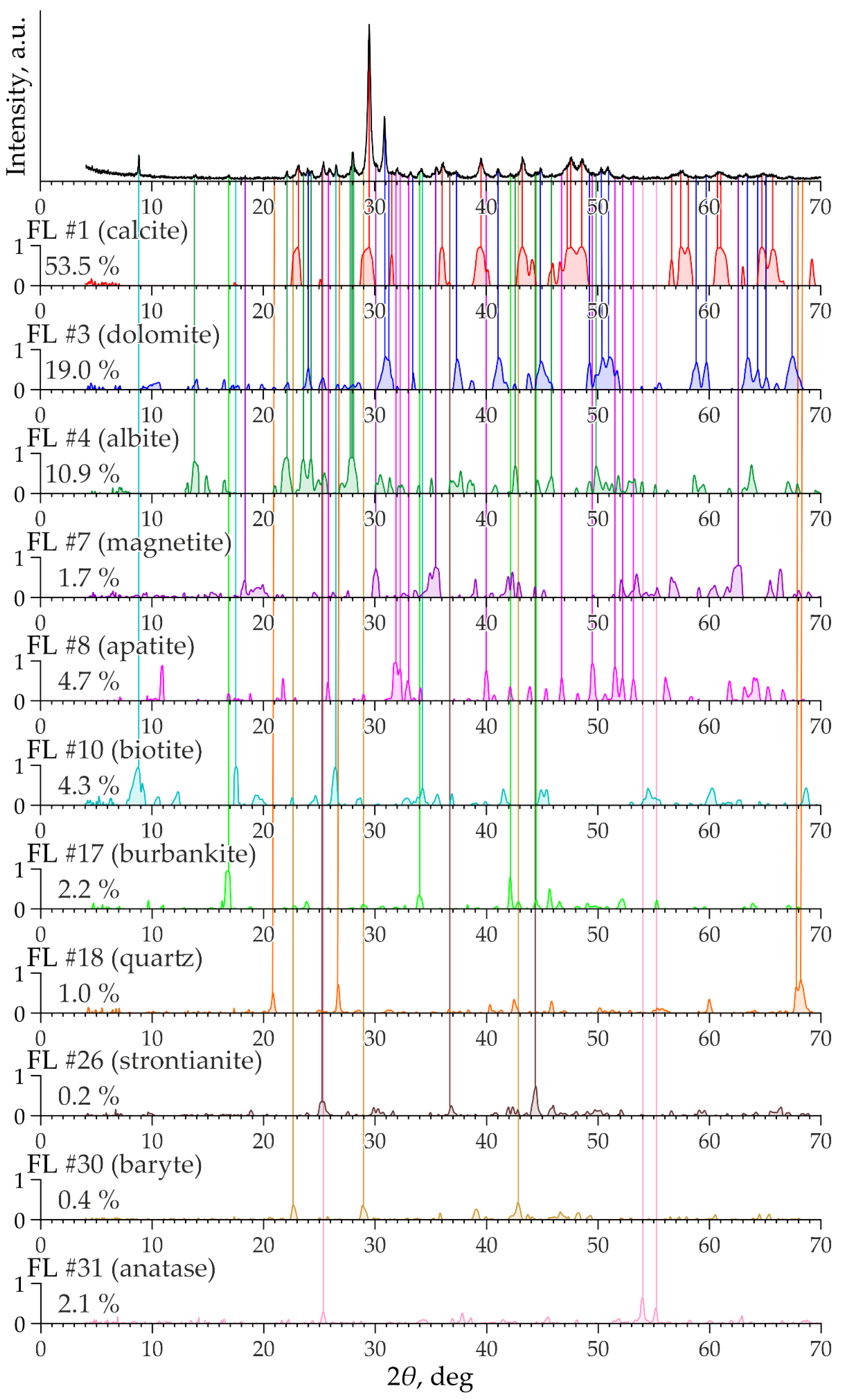
4.1. Types of the Extracted Factors

Data processing of the Kontozero collection yielded 107 factors, describing a 100% dispersion of the raw data. Analysis of the FL graphs showed that more than a third of the obtained factors describe the noise component (Figure 3). The graphs of the noise factors have no distinct peaks but contain many “outliers” (single points with high FL values surrounded by those with low FL values). Therefore, we excluded all these factors from consideration.

About a third of FL graphs have either one intense peak or a series of low-intensity peaks (Figure 4). Factors with these FL graphs are interpretable only in exceptional cases (when analyzing them, we used the techniques described below, in most cases to no avail). Note that, altogether, factors of this type explain less than 10% of the data dispersion.

Only the remaining third of the factors, which showed many distinct peaks on FL graphs (Figure 5), turned out to be informative. This group includes mainly the first 30 factors that altogether account for 90% of the total data dispersion. We focus on these factors below, because they were subject to mineralogical interpretation.

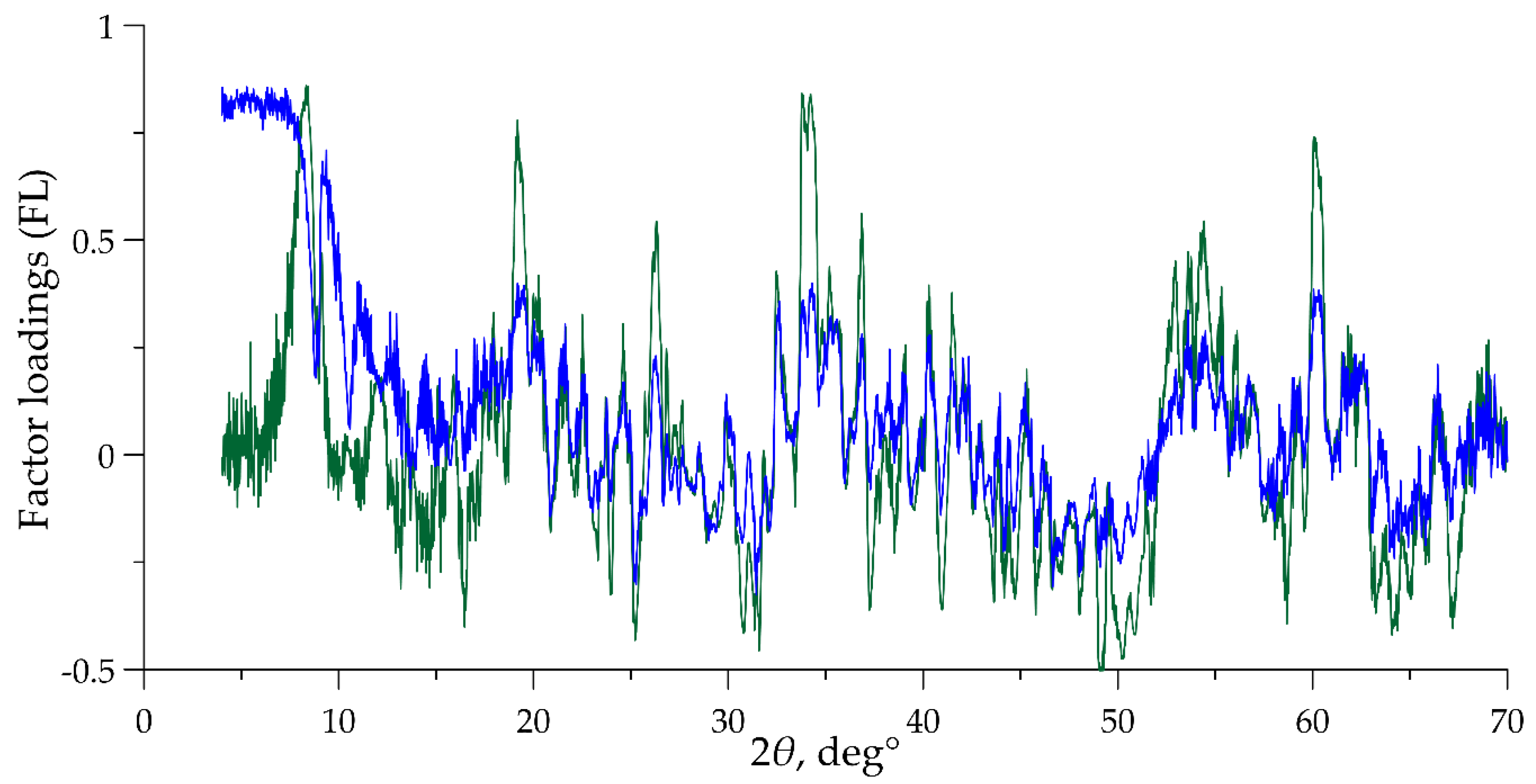
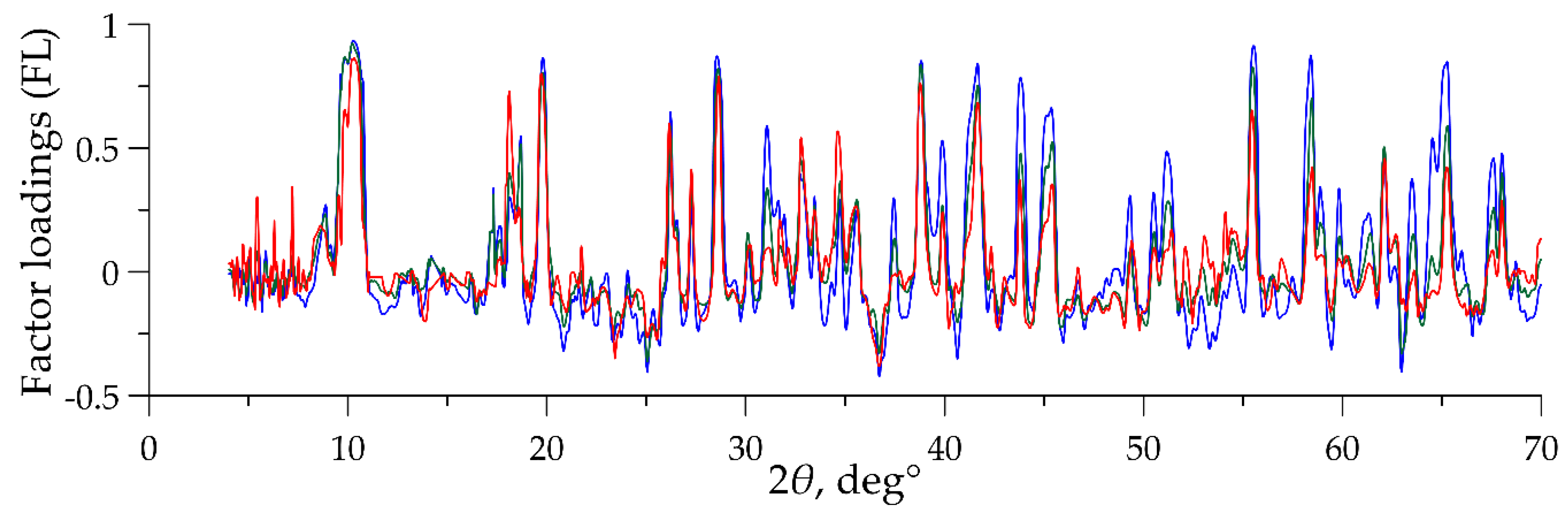
4.2. Evaluation of the Stability of the Factor Solution

To evaluate the stability of the obtained solution, we conducted two additional numerical experiments.

First, it was necessary to check whether the performed operations with the spectra (baseline correction and smoothing) affected the result. Therefore, we compared the FA results for the following three datasets:

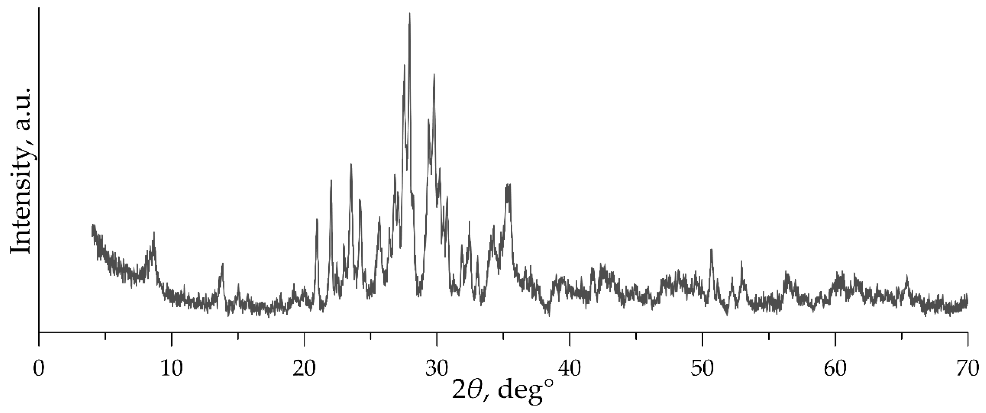
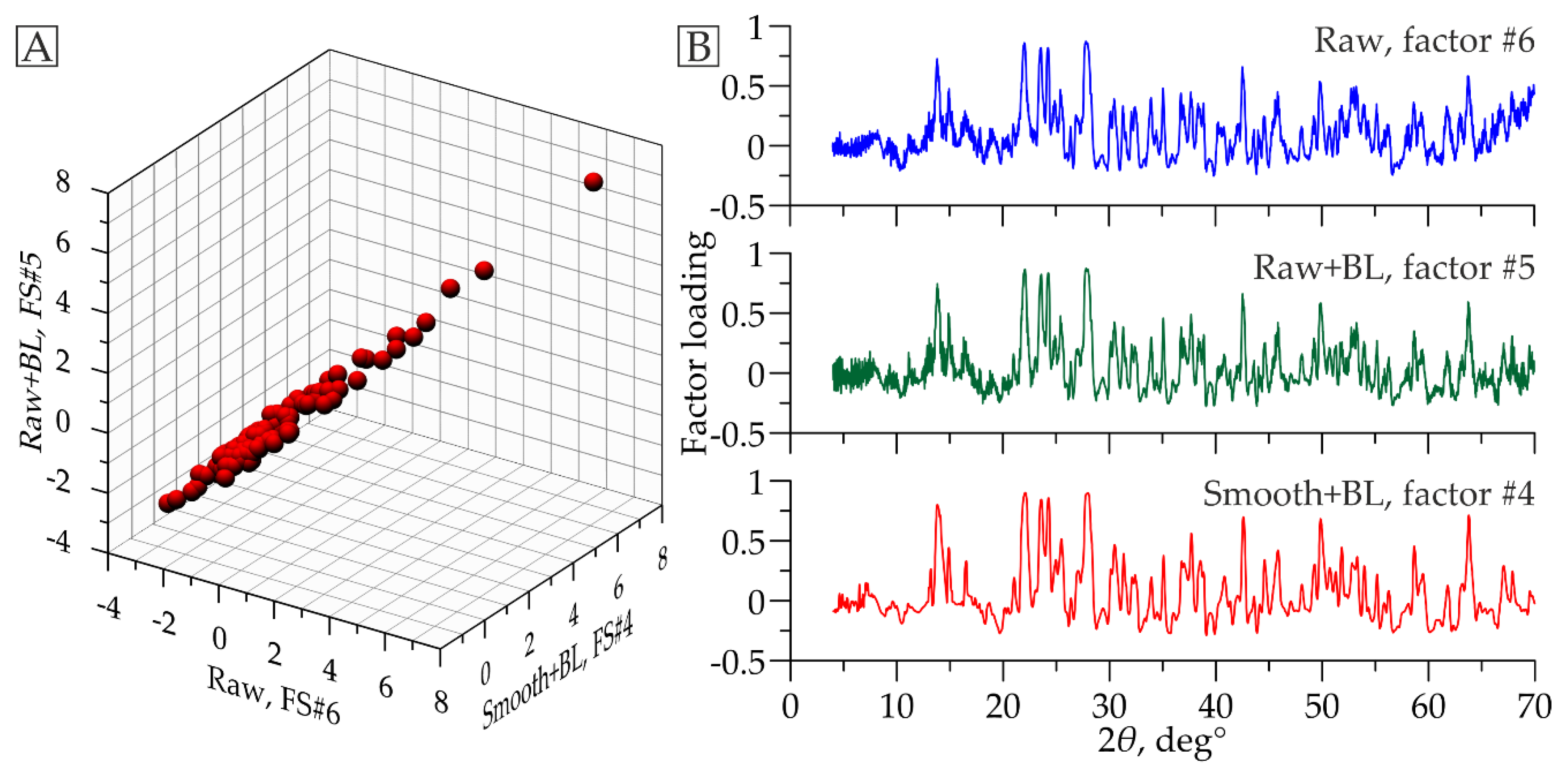
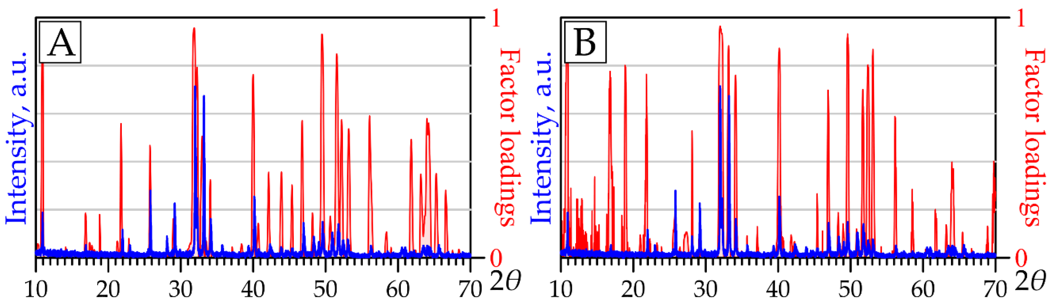
• Raw X-ray diffraction patterns not subjected to any spectral operations;
• Raw diffraction patterns subjected to baseline correction;
• Smoothed diffraction patterns subjected to baseline correction (the data used in the method of [13]).

As a result, we obtained three sets of factors. For the overwhelming majority of interpreted factors from each set, analogs were found among the factors of other sets. The similarity is distinct both in the high values of the correlation coefficient between FSs (

Table 1. The correlation coefficients between scores of similar factors resulting from factor analysis (FA) of the X-ray powder diffraction (XRPD) datasets subjected to different spectral operations.

Raw data (factors #):	1 *	2	3	4	5	6	7	8	9
Raw data + baseline (factors #):	1	2	3	4	7	5	6	8	9
Correlation coefficient between FSs:	0.91	0.94	0.43	0.97	0.97	0.97	0.94	0.97	0.97
Raw data (factors #):	1	2	3	4	5	6	7	8	9
Smoothed data + baseline (factors #):	1	2	11	5	6	4	7	9	8
Correlation coefficient between FSs:	0.76	0.89	0.20	0.94	0.96	0.95	0.87	0.94	0.95

* Factor numbers correspond to the rank in a series arranged in descending order of the data dispersion explained by the factor.

, Figure 6A) and in the identity of the FL graphs (Figure 6B).

The difference in the serial numbers of analogous factors in the considered sets (see Table 1) is due to differences in the volumes of data dispersion explained by these factors. For instance, the factor shown as an example in Figure 6 explains 3.0% of the dispersion of the dataset composed of raw diffraction patterns. In the case of raw diffractograms with baseline correction, it accounts for 3.4% of data dispersion. Lastly, it explains 6.9% of the dispersion for a database on smoothed diffraction patterns. As a result, the factor under consideration has the ordinal number #6 in the first set of factors, #5 in the second set, and #4 in the third set. Typically, differences in the explained dispersion are small, and permutations occur in the immediate position (see Table 1).

Against the background of the considered analogous factors, a specific factor #3, extracted from the dataset of raw diffraction patterns, stands out. First, the FL graphs of its closest analogs from the results of processing other datasets have only a distant similarity with the FL graph of this factor (Figure 7). The FSs of all these factors are poorly correlated (see Table 1). Second, on the FL graph of factor #3, in addition to sharp peaks, a broad maximum occurs in the range of small 2θ angles. All diffraction patterns used in this study are bent to the top in this area (see Figure 2). This artifact disappears after the baseline correction procedure. Hence, the specificity of factor #3, extracted from raw diffraction patterns, is due to the information on the background component contained therein.

Thus, our analysis showed that, in theory, even raw data are appropriate for research. However, if no baseline correction is made, additional factors overloaded by supplementary background information appear, which complicates the interpretation of the FA results. On the contrary, diffractogram smoothing, combined with baseline correction, simplifies the interpretation. The FL graphs obtained after such spectral manipulations are devoid of the outliers typical of raw data processing results (see Figure 6B). Nevertheless, FL graphs retain all the nuances of morphology. It follows that the performed spectral operations do not distort the information contained in the XRPD, and do not affect the results of FA.

The second numerical experiment we conducted aimed to determine whether the result of FA is particular or general. By a “particular” result, we refer to its relation to the tested sample subset (the working hypothesis implies that different sample subsets can yield different factor solutions). By a “general” result, we mean a solution resistant to any rearrangement of samples.

In this numerical experiment, we subjected the following three datasets to FA:

• The subset of carbonatites sensu stricto selected according to the formal principle “SiO₂ < 20 wt %”, commonly used for the classification of carbonatites [36]—99 observations;
• The cumulative subset of all other rocks of the collection (silicocarbonatites and carbonate-bearing silicate rocks)—99 observations;
• The entire set of samples from the Kontozero collection—198 observations.

After processing these datasets, as in the previous experiment, we revealed many analogous factors characterized by very similar FL graphs (Figure 8). Thus, the result of processing XRPD data with the FA represents a robust general solution. This solution is determined solely by the specifics of the mineral composition. It only requires the samples to be representative (that is, the set of samples must contain all mineral phases characteristic of the object of study).

4.3. Interpretation of the Results of Factor Analysis

After the stability of the solution obtained with the FA was proven, we proceeded to interpret the results. This procedure involves the decryption of the information hidden in the parameters of FL and FS. The positions of peaks on the FL graphs of the factors chosen for interpretation (see Section 4.1) coincide with the positions of the corresponding peaks on the diffractograms of certain minerals from the databases. For example, intense peaks in the FL graph of one of the factors occur at the same 2θ as in the fluorapatite diffractogram from the RRUFF database [37] (Figure 9A). Note that a similar FL graph was observed when studying the carbonatites of the Petyayan-Vara area (Vuoriyarvi massif, NW Russia) [13] (Figure 9B).

We compared the FL graphs and the diffraction patterns of those samples in which the FSs of the corresponding factors were the highest (i.e., the highest expected content of the mineral associated with a factor [38]). Visual comparison of graphs (Figure 10A) in all considered cases was effective and sufficient. However, comparison can also be formalized mathematically. For this procedure, it is necessary to construct a ranked range of FL values and analyze it using the methodology similar to the “Cattell’s scree test” [39], which is often utilized in FA to determine the number of interpreted factors. The essence is to identify the inflection point on the ranked range, after which the dynamics of decreasing values changes (Figure 10B). This procedure allows us to identify the most significant peaks on FL graphs (i.e., those whose FL values exceed the FL value of the inflection point) and to compare the diffraction patterns with only them (Figure 10C). Mention should be made of the critical FL value, which can be estimated using standard statistical tests. Below this critical value, FL loses its statistical significance (for 198 samples, the critical value modulus is 0.18 at the significance level of p = 0.01).

For many factors, the most intense peaks in the FL plots coincided with several pronounced peaks in the diffraction patterns (Figure 10A). For a mineralogical explanation of these factors, we used two techniques: (1) a mineral search in the online XRPD AMCSD database [32] using the “Diffraction Search” tool for the most intense peaks in the FL, with the “Tolerance” parameter equal to 0.1 (Figure 10B); and (2) qualitative identification of the phase of interest in the diffraction pattern of the sample with the maximum FS using the QualX v. 2.24 program [30] (via the peaks simultaneously occurring in both the diffractogram and the FL graph; see Figure 10C).

It should be borne in mind that in cases where the contents of some minerals in the rocks are close to proportional, these minerals can be combined into one factor [13]. During this study, we also observed peaks of several minerals (for example, magnetite and diopside) as part of a single FL graph of factor loadings. Given the possibility of “mixing” several minerals into one factor, the analysis of diffraction patterns with maximum FSs is preferable. However, it is technically more complex, and we achieved the best results by combining both interpretation techniques.

The analysis of FLs on geochemical variables (

Table 2. Factor loadings of geochemical variables for some interpretable factors.

	1 *	2	3	4	5	6	7	8	9	10	17	22	24	26	30	31
	Cal **	Adr + Srp	Dol	Ab	Amp	Anl	Di + Mag	Ap	Or	Bt	Bur	Py	Ilm	Str	Brt	Ant
Si	−0.71	0.19	−0.15	0.29	0.14	0.24	0.22	−0.15	0.24	0.11	−0.05	0.05	0.08	−0.05	−0.05	0.03
Ti	−0.67	0.24	−0.14	0.05	−0.02	0.17	0.05	−0.24	0.04	0.23	−0.07	0.10	0.20	−0.04	−0.05	0.15
Zr	−0.30	−0.09	−0.09	0.29	−0.11	0.48	−0.05	0.19	0.34	−0.01	−0.05	0.15	0.13	−0.07	−0.04	0.08
Al	−0.53	0.00	−0.15	0.53	−0.11	0.38	−0.04	−0.15	0.35	0.07	0.00	0.05	0.08	−0.05	−0.04	0.06
Ca	0.83	−0.09	0.01	−0.19	−0.17	−0.16	−0.21	0.13	−0.13	−0.14	0.05	−0.05	−0.07	0.06	0.06	−0.04
Sr	0.59	−0.23	0.01	−0.01	−0.24	−0.10	−0.29	−0.05	−0.08	−0.18	0.22	−0.08	−0.03	0.36	0.06	−0.08
Mg	−0.55	0.32	0.07	−0.29	0.32	−0.10	0.35	−0.08	−0.21	0.17	−0.07	0.01	0.02	−0.05	−0.04	−0.01
Fe	−0.78	0.19	−0.13	−0.04	0.08	0.06	0.41	0.04	−0.06	0.10	−0.07	0.03	0.04	−0.12	−0.08	0.02
Mn	−0.55	0.07	−0.08	−0.12	0.21	−0.09	0.23	0.08	−0.13	0.04	0.09	−0.07	−0.13	0.02	−0.02	−0.20
Ba	−0.19	−0.14	−0.10	0.03	−0.13	0.04	−0.25	−0.12	0.15	−0.03	0.08	−0.04	−0.03	0.20	0.25	−0.04
K	−0.47	−0.13	−0.20	0.13	−0.05	0.12	−0.05	−0.15	0.66	0.19	−0.09	0.06	0.04	−0.06	−0.03	0.07
Na	−0.51	−0.19	0.08	0.56	0.26	0.42	−0.01	−0.07	0.02	0.04	0.07	0.00	0.07	−0.09	−0.03	0.04
P	−0.07	−0.08	−0.08	−0.13	−0.07	−0.02	−0.06	0.95	−0.07	−0.02	0.06	0.09	−0.01	−0.05	−0.02	−0.01
S	−0.20	−0.14	0.16	0.05	−0.19	−0.05	−0.29	0.24	0.02	−0.03	−0.11	0.67	−0.01	−0.05	−0.02	0.01
L.O.I.	0.75	−0.27	0.26	−0.12	−0.07	−0.20	−0.25	−0.09	−0.10	−0.13	0.06	−0.02	−0.14	−0.08	0.00	0.07

* Factor number. ** Mineralogical interpretation: Ab—albite; Adr—andradite; Amp—amphibole; Anl—Analcime; Ant—anatase; Ap—apatite; Brt—baryte; Bt—biotite; Bur—burbankite; Cal—calcite; Di—diopside; Dol—dolomite; Ilm—ilmenite; Mag—magnetite; Or—orthoclase; Py—pyrite; Srp—serpentine; and Str—strontianite. The statistically significant loadings are in bold (p = 0.01).

) additionally illustrated the mineralogical nature of the factors. There is a clear pattern in the attribution of the maximum FLs: Ca (0.83) and L.O.I. (0.75) for calcite factor; Na (0.56) and Al (0.53) for albite factor; Fe (0.41) and Mg (0.35) for the factor combining magnetite and diopside; P (0.95) for apatite factor; K (0.66) for orthoclase factor; S (0.67) for pyrite factor, etc. (the analysis of geochemical FLs is detailed in [13]).

The described methods identified about 20 factors associated with 21 minerals: Ca-Mg-Fe carbonates (calcite, ferruginous dolomite, and siderite); strontianite; feldspars (orthoclase and albite); garnet (andradite); monticellite; diopside; biotite; chlorite; serpentine; zeolites (natrolite and analcime); quartz; magnetite; ilmenite; fluorite; fluorapatite; pyrite; and anatase. Subsequently, we found all these phases by electron probe microanalysis (EPMA) in thin sections of samples identified by the FA as a priority for their high FSs (Figure 11).

In addition, we extracted several specific factors with intense peaks in FL graphs. Diffraction patterns of samples with maximum FSs of these factors in the corresponding regions have only weak lines and/or lines overlapped by lines of other minerals (e.g., Figure 12A,B). For such factors, the qualitative identification of the phase of interest by the diffractogram with the maximum FS is not practical. Thus, we diagnosed these factors based on the position of the most intense peaks in the AMCSD database. The subsequent mineralogical study of samples with maximum FSs confirmed our assumptions. Ultimately, a comparison with the identified factors revealed several minerals in the studied rocks, which, although not abundant, are of significant petrological interest. The examples are burbankite (Na,Ca)₃(Sr,Ba,Ce)₃(CO₃)₅ (Figure 12C) and baryte (Figure 12D). Their diffractograms do not contain pronounced peaks due to the low content of these minerals in the rocks (up to several wt%). However, the proposed technique turned out to be sensitive even to these accessory phases.

4.4. The Algorithm for the Selection of Representative Samples

Summarizing the results of this study, we propose the following algorithm for selecting the most representative samples in an extensive collection of rocks of a geological object:

• XRPD and XRF analysis and primary data processing, including baseline corrections and removal of zero values. The output of this step is a database suitable for FA (an example is shown in the supplementary Table S3);
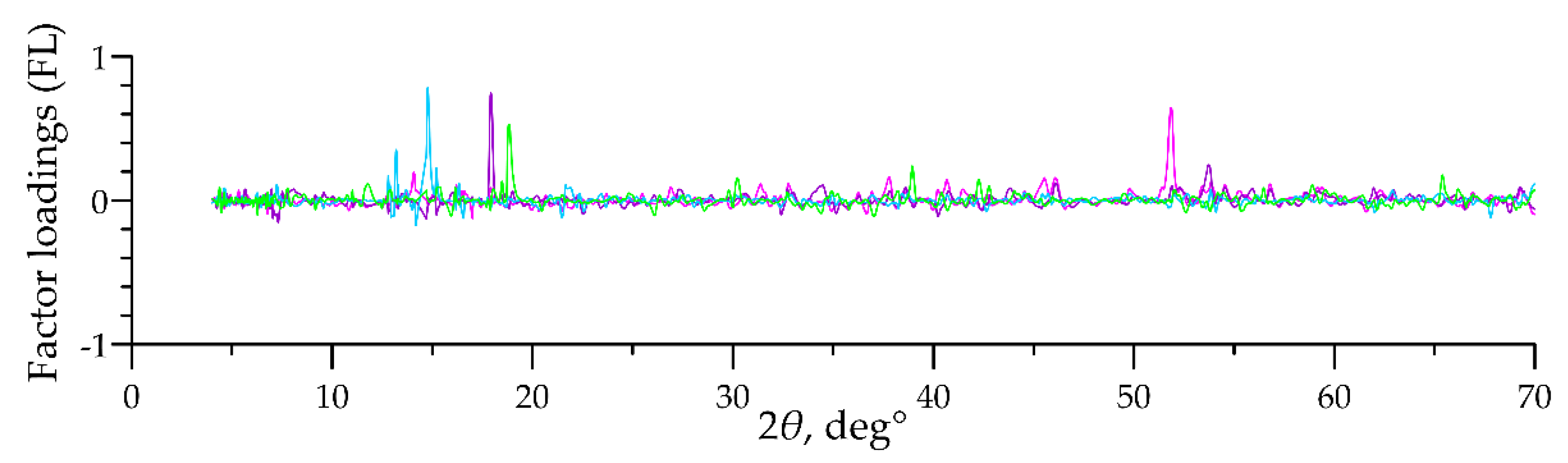
• Factor analysis of the obtained results. The outputs are (a) tables of FL values for XRPD and XRF variables (see Supplementary Table S4), (b) graphs of factor loadings for XRPD variables (e.g., Figure 5), and (c) factor scores for each sample (see Supplementary Table S5);
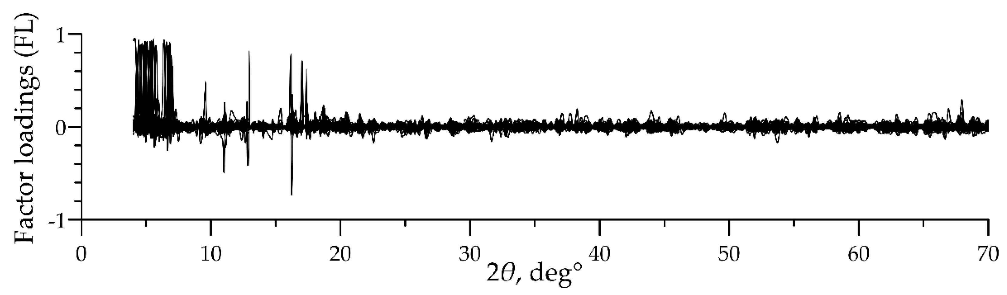
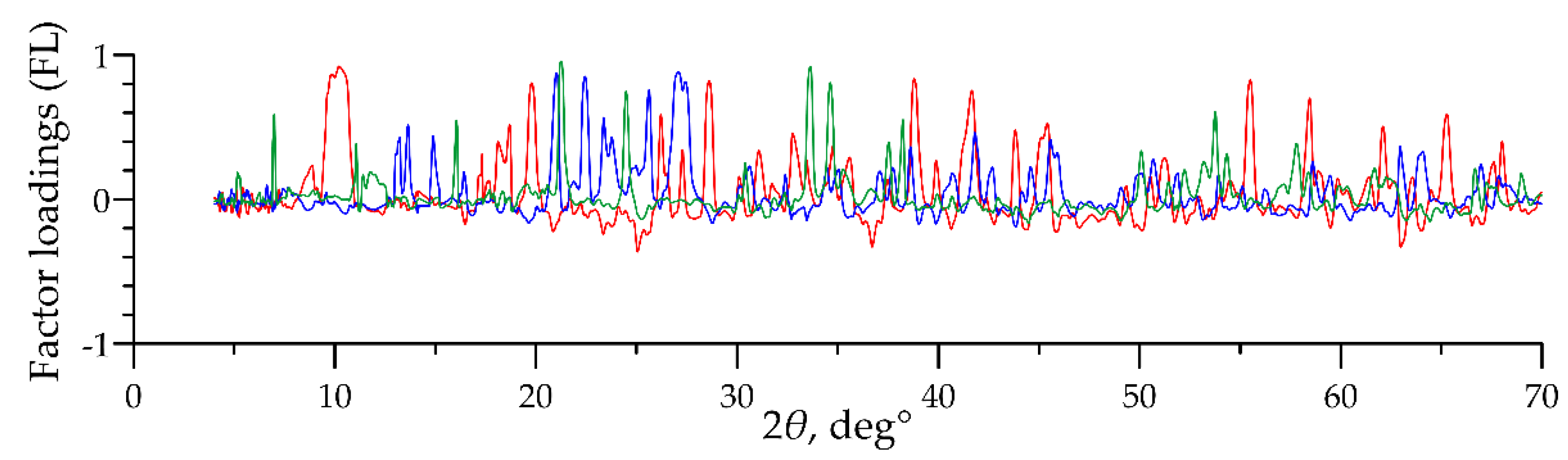
• Compilation and examination of all FL graphs on a single chart. The output is the rejection of all non-interpreted noise factors (see Figure 3);
• Comparison of each factor graph with the diffraction pattern of the sample, which shows the maximum score value of this factor. The output is a division of factors into easy to interpret (e.g., Figure 10A) and difficult to interpret (e.g., Figure 12A);
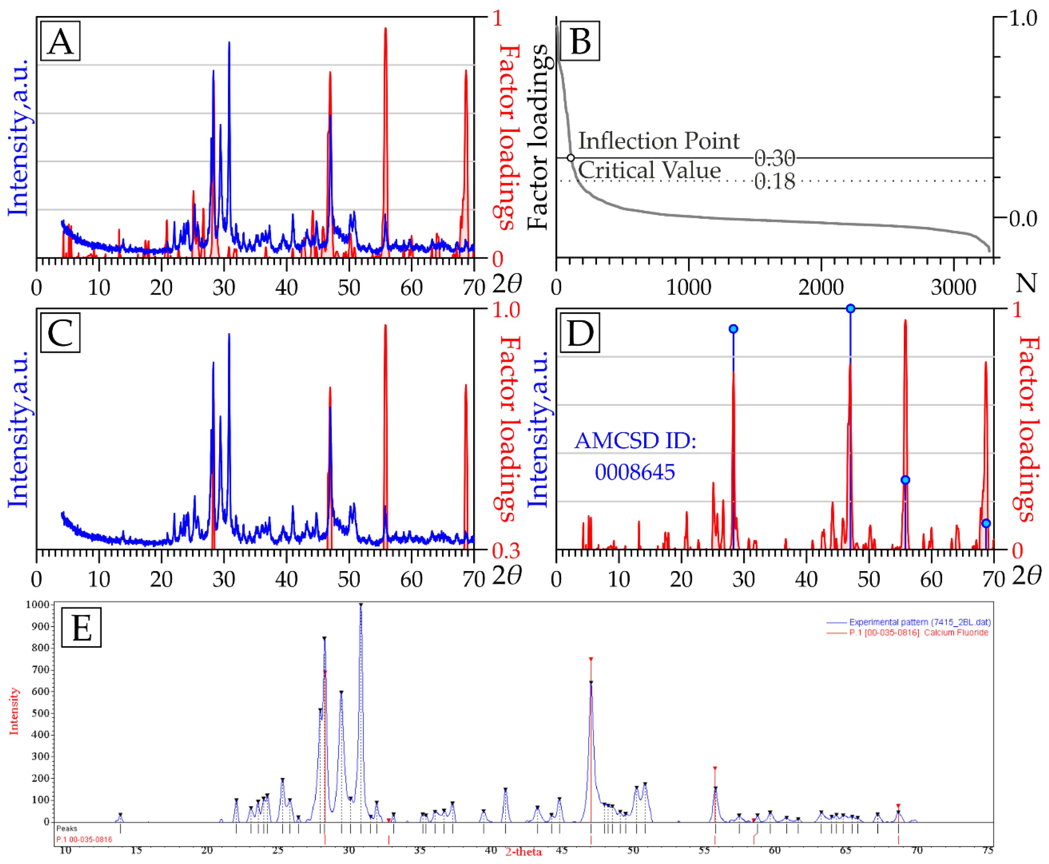
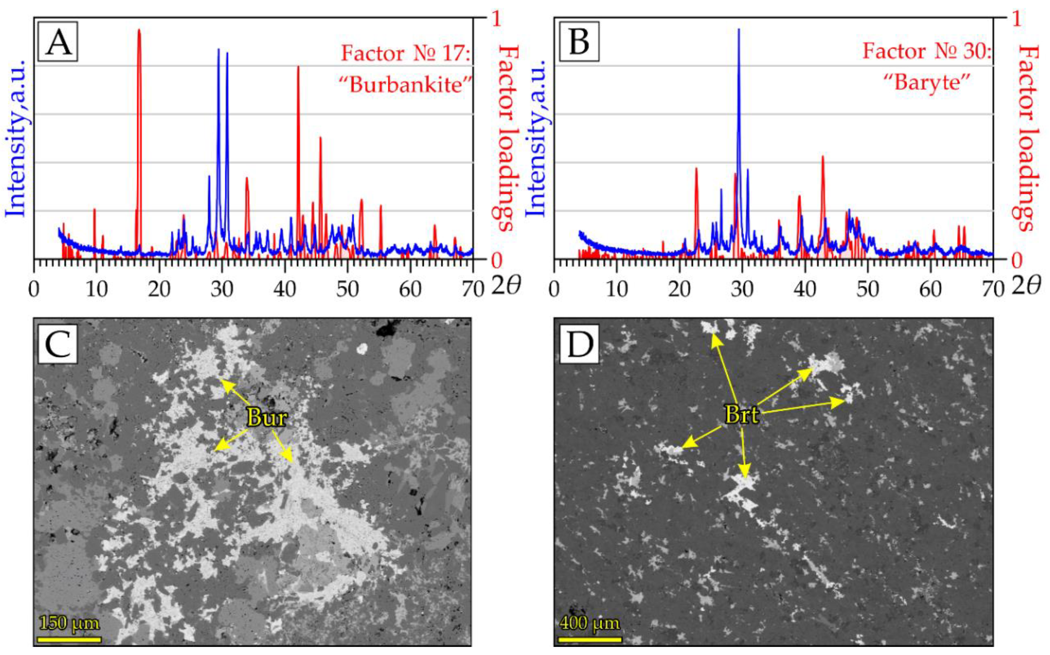
• Interpretation of the easily interpretable factors by combining the two proposed techniques (Figure 10). The output is a highly confident mineralogical explanation of these factors;
• Interpretation of difficult-to-interpret factors by searching for the mineral (s) according to the position of the most intense peaks in the AMCSD database. The output is an assumption about the nature of these factors;
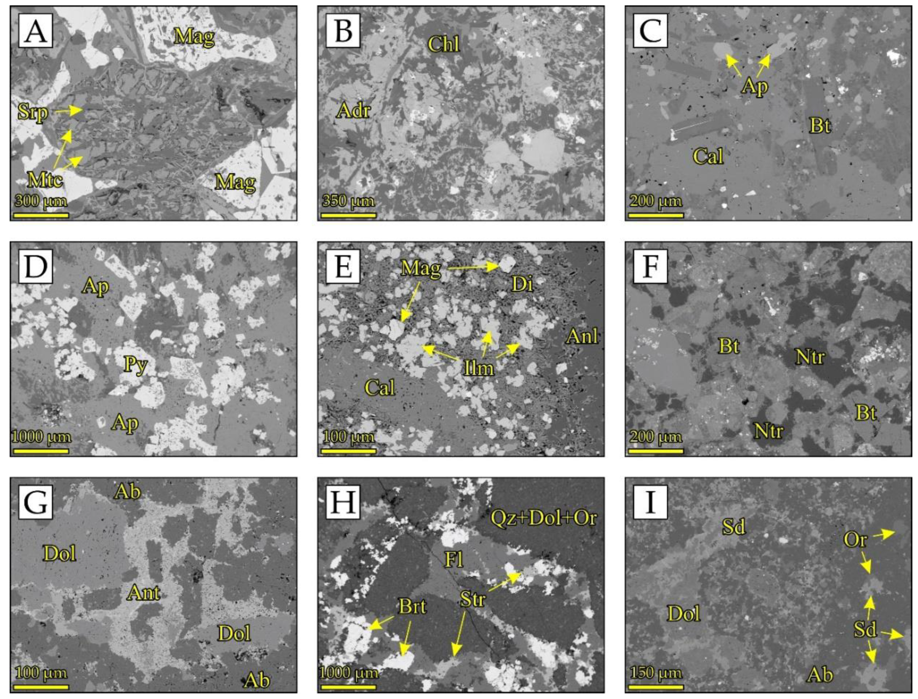
• Routine mineralogical (optical microscopy, SEM + EPMA, Raman) examination of the samples with the highest FSs. The output is a verification of the FA results, a collection of the most representative samples, an idea of the mineral composition of all studied rocks at the level of main, minor, and most accessory minerals, all within a reasonably short time.

5. Conclusions and Future Perspectives

The proposed FA-based technique ascribed a large and unwieldy set of original data on the rocks of Kontozero to a small set of factors. The number of factors was minimized to the extent necessary to represent all non-random differences in the combined (XRPD + XRF) dataset. After this analysis, all the relevant information remained in full, which was confirmed by numerical modeling that proved the stability of the factor solution. The factor loading graphs of many extracted factors show pronounced peaks that coincide in position with the lines on the diffraction patterns of the samples. This phenomenon makes it possible to carry out mineralogical identification of factors using two techniques: (1) based on the graphs of factor loadings and (2) based on the diffraction patterns of samples with the maximum factor score. The first technique also reveals phases that do not yield pronounced peaks in the diffractograms, owing to their low content in the rocks. We note that in the latter case, additional methods of mineral diagnostics are required. In sum, the results of this study allowed us to develop an algorithm for selecting the most representative samples with the highest contents of certain minerals.

Further prospects for the discussed methodology include an in-depth assessment of the impact of noise and the possibility of its quantification; determining the impact of pre-treatment of XRPD data on the FA result; FA-based investigation of XRPD datasets with wider 2θ ranges (up to 100 ° or more) and determination of data range effects; examination of the influence of characteristics distorting the primary XRPD data (primarily the preferred orientation of crystallites) on the FA result and an assessment of the robustness of the proposed technique to these factors; comparison of the results of factor and cluster analyzes of the same XRPD-dataset and determining possible ways of their joint complementary use; the use of several FA and similar techniques (PCA, independent component analysis, etc.), allowing to limit the result, for example, non-negative matrix factorization [10].

References

1. Olympus. XRF and XRD Analyzers. Available online: https://www.olympus-ims.com/en/innovx-xrf-xrd/ (accessed on 19 August 2020).
2. Xu, X.; Liang, T.; Zhu, J.; Zheng, D.; Sun, T. Review of classical dimensionality reduction and sample selection methods for large-scale data processing. Neurocomputing 2019, 328, 5–15. [Google Scholar] [CrossRef]
3. Mirzaei-Paiaman, A.; Asadolahpour, S.R.; Saboorian-Jooybari, H.; Chen, Z.; Ostadhassan, M. A new framework for selection of representative samples for special core analysis. Pet. Res. 2020. [Google Scholar] [CrossRef]
4. Barr, G.; Dong, W.; Gilmore, C.J. PolySNAP: A computer program for analysing high-throughput powder diffraction data. J. Appl. Crystallogr. 2004, 37, 658–664. [Google Scholar] [CrossRef] [Green Version]
5. Barr, G.; Dong, W.; Gilmore, C. PolySNAP3: A computer program for analysing and visualizing high-throughput data from diffraction and spectroscopic sources. J. Appl. Crystallogr. 2009, 42, 965–974. [Google Scholar] [CrossRef]
6. Butler, B.M.; Palarea-Albaladejo, J.; Shepherd, K.D.; Nyambura, K.M.; Towett, E.K.; Sila, A.M.; Hillier, S. Mineral–nutrient relationships in African soils assessed using cluster analysis of X-ray powder diffraction patterns and compositional methods. Geoderma 2020, 375, 114474. [Google Scholar] [CrossRef]
7. Butler, B.M.; Sila, A.M.; Shepherd, K.D.; Nyambura, M.; Gilmore, C.J.; Kourkoumelis, N.; Hillier, S. Pre-treatment of soil X-ray powder diffraction data for cluster analysis. Geoderma 2019, 337, 413–424. [Google Scholar] [CrossRef]
8. Chen, Z.P.; Morris, J.; Martin, E.; Hammond, R.; Lai, X.; Ma, C.; Purba, E.; Roberts, K.J.; Bytheway, R. Enhancing the Signal-to-Noise Ratio of X-ray Diffraction Profiles by Smoothed Principal Component Analysis. Anal. Chem. 2005, 77, 6563–6570. [Google Scholar] [CrossRef]
9. Wasserman, S.R.; Allen, P.G.; Shuh, D.K.; Bucher, J.J.; Edelstein, N.M. EXAFS and principal component analysis: A new shell game. J. Synchrotron Radiat. 1999, 6, 284–286. [Google Scholar] [CrossRef] [Green Version]
10. Liu, P.; Zhou, X.; Li, Y.; Li, M.; Yu, D.; Liu, J. The application of principal component analysis and non-negative matrix factorization to analyze time-resolved optical waveguide absorption spectroscopy data. Anal. Methods 2013, 5, 4454–4459. [Google Scholar] [CrossRef]
11. Frenkel, A.I.; Kleifeld, O.; Wasserman, S.R.; Sagi, I. Phase speciation by extended X-ray absorption fine structure spectroscopy. J. Chem. Phys. 2002, 116, 9449–9456. [Google Scholar] [CrossRef] [Green Version]
12. Burley, J.C.; O’Hare, D.; Williams, G.R. The application of statistical methodology to the analysis of time-resolved X-ray diffraction data. Anal. Methods 2011, 3, 814. [Google Scholar] [CrossRef]
13. Fomina, E.; Kozlov, E.; Ivashevskaja, S. Study of diffraction data sets using factor analysis: A new technique for comparing mineralogical and geochemical data and rapid diagnostics of the mineral composition of large collections of rock samples. Powder Diffr. 2019, 34, S59–S70. [Google Scholar] [CrossRef]
14. George, D. IBM SPSS Statistics 23 Step by Step; Routledge: New York, NY, SUA, 2016; ISBN 9781315545899. [Google Scholar]
15. Wold, S.; Esbensen, K.; Geladi, P. Principal component analysis. Chemom. Intell. Lab. Syst. 1987, 2, 37–52. [Google Scholar] [CrossRef]
16. Ford, W. The Singular Value Decomposition. In Numerical Linear Algebra with Applications Using MATLAB; Ford, W., Ed.; Academic Press: Boston, MA, USA, 2015; pp. 299–320. ISBN 978-0-12-394435-1. [Google Scholar]
17. Klug, H.P.; Alexander, L.E. X-ray Diffraction Procedures for Polycrystalline and Amorphous Materials; John Wiley & Sons, Inc.: New York, NY, USA, 1954. [Google Scholar]
18. Jenkins, R.; Snyder, R.L. Introduction to X-ray Powder Diffractometry; John Wiley & Sons, Inc.: Hoboken, NJ, USA, 1996; ISBN 9781118520994. [Google Scholar]
19. MAUD Software. Available online: http://maud.radiographema.eu/ (accessed on 3 July 2020).
20. Lutterotti, L.; Matthies, S.; Wenk, H.-R. MAUD: A friendly Java program for materials analysis using diffraction. Int. Union Crystallogr. Comm. Powder Diffr. Newsl. 1999, 21, 14–15. [Google Scholar]
21. Downes, H.; Balaganskaya, E.; Beard, A.; Liferovich, R.; Demaiffe, D. Petrogenetic processes in the ultramafic, alkaline and carbonatitic magmatism in the Kola Alkaline Province: A review. Lithos 2005, 85, 48–75. [Google Scholar] [CrossRef] [Green Version]
22. Bulakh, A.; Ivanikov, V.; Orlova, M.; Wall, F. Overview of carbonatite-phoscorite complexes of the Kola Alkaline Province in the context of a Scandinavian North Atlantic Alkaline Province. In Phoscorites and Carbonatites from Mantle to Mine; Wall, F., Zaitsev, A.N., Eds.; Mineralogical Society of Great Britain and Ireland: London, UK, 2004; pp. 1–43. [Google Scholar]
23. Kramm, U.; Kogarko, L.; Kononova, V.; Vartiainen, H. The Kola Alkaline Province of the CIS and Finland: Precise Rb-Sr ages define 380–360 Ma age range for all magmatism. Lithos 1993, 30, 33–44. [Google Scholar] [CrossRef]
24. Arzamastsev, A.A.; Petrovsky, M.N. Alkaline volcanism in the Kola Peninsula, Russia: Paleozoic Khibiny, Lovozero and Kontozero calderas. Proc. MSTU 2012, 15, 277–299. [Google Scholar]
25. Petrovsky, M.N.; Savchenko, E.A.; Kalachev, V.Y. Formation of eudialyte-bearing phonolite from Kontozero carbonatite paleovolcano, Kola Peninsula. Geol. Ore Deposits 2012, 54, 540–556. [Google Scholar] [CrossRef]
26. Website of IM UB RAS (Miass, Russia). Available online: http://www.mineralogy.ru (accessed on 3 July 2020).
27. Amosova, A.A.; Panteeva, S.V.; Chubarov, V.M.; Finkelshtein, A.L. Determination of major elements by wavelength-dispersive X-ray fluorescence spectrometry and trace elements by inductively coupled plasma mass spectrometry in igneous rocks from the same fused sample (110 mg). Spectrochim. Acta Part B At. Spectrosc. 2016, 122, 62–68. [Google Scholar] [CrossRef]
28. Website of IG SB RAS (Irkutsk, Russia). Available online: http://www.igc.irk.ru (accessed on 3 July 2020).
29. Qualx2 Software. Available online: http://www.ba.ic.cnr.it/softwareic/qualx/ (accessed on 3 July 2020).
30. Altomare, A.; Corriero, N.; Cuocci, C.; Falcicchio, A.; Moliterni, A.G.G.; Rizzi, R. QUALX2.0: A qualitative phase analysis software using the freely available database POW_COD. J. Appl. Crystallogr. 2015, 48, 598–603. [Google Scholar] [CrossRef]
31. Kaiser, H.F. The varimax criterion for analytic rotation in factor analysis. Psychometrika 1958, 23, 187–200. [Google Scholar] [CrossRef]
32. Downs, R.T.; Hall-Wallace, M. The American Mineralogist crystal structure database. Am. Mineral. 2003, 88, 247–250. [Google Scholar]
33. Gražulis, S.; Daškevič, A.; Merkys, A.; Chateigner, D.; Lutterotti, L.; Quirós, M.; Serebryanaya, N.R.; Moeck, P.; Downs, R.T.; Le Bail, A. Crystallography Open Database (COD): An open-access collection of crystal structures and platform for world-wide collaboration. Nucleic Acids Res. 2011, 40, D420–D427. [Google Scholar] [CrossRef] [PubMed]
34. Gates-Rector, S.; Blanton, T.N. The Powder Diffraction File: A quality materials characterization database. Powder Diffr. 2019, 34, 352–360. [Google Scholar] [CrossRef] [Green Version]
35. Fomina, E.; Kozlov, E. Application of the method of statistical comparison of XRD- and XRF-data for identification of the most representative rоск samples: Case study of a large collection of carbonatites and aluminosilicate rocks of the Kontozero alkaline complex (Kola Peninsula, NW Russia). IOP Conf. Ser. Earth Environ. Sci. 2020, in press. [Google Scholar]
36. Le Maitre, R.W.; Streckeisen, A.; Zanettin, B.; Le Bas, M.J.; Bonin, B.; Bateman, P.; Bellieni, G.; Dudek, A.; Efremova, S.; Keller, J.; et al. Igneous Rocks, 2nd ed.; Le Maitre, R.W., Streckeisen, A., Zanettin, B., Le Bas, M.J., Bonin, B., Bateman, P., Eds.; Cambridge University Press: Cambridge, UK, 2002; ISBN 9780511535581. [Google Scholar]
37. Lafuente, B.; Downs, R.T.; Yang, H.; Stone, N.L. The power of databases: The RRUFF project. In Highlights in Mineralogical Crystallography; Armbruster, T., Danisi, R.M., Eds.; De Gruyter: Berlin/München, Germany, 2016; pp. 1–30. ISBN 9783110417104. [Google Scholar]
38. Kozlov, E.; Fomina, E.; Khvorov, P. Factor Analysis of XRF- and XRPD-data on the Example of the Rocks of the Kontozero Carbonatite Complex (NW Russia). Part II: Geological Interpretation. Crystals 2020, 10, 873. [Google Scholar] [CrossRef]
39. Cattell, R.B. The Scree Test For The Number Of Factors. Multivariate Behav. Res. 1966, 1, 245–276. [Google Scholar] [CrossRef]
Figure 1. Comparison of the diffraction pattern of an exemplary sample with the factor loading (FL) graphs of factors of the minerals constituting this sample (quantitative analysis was performed using the MAUD program [19,20]).
Crystals 10 00874 g001
Figure 2. A typical diffraction pattern used in this study.
Crystals 10 00874 g002
Figure 3. The factor loadings (FL) graphs of the noise factors (42 out of 107 factors). Figure 3 is taken from [35].
Crystals 10 00874 g003
Figure 4. Examples of FL graphs of uninterpretable factors.
Crystals 10 00874 g004
Figure 5. Examples of FL graphs of the most informative factors (red line—factor #5 “alkaline amphibole”; blue line—factor #9 “orthoclase”; green line—factor #12 “monticellite”).
Crystals 10 00874 g005
Figure 6. (A) An example of a robust linear relationship between the factor score (FS) values of analogous factors resulting from factor analysis of three XRPD datasets: “Raw”—raw data without spectral operations; “Raw + BL”—raw data with baseline correction; “Smooth + BL”—smoothed data with baseline correction. (B) Comparison of factor loadings graphs of the same factors.
Crystals 10 00874 g006
Figure 7. Comparison of the FL graphs of a specific factor, containing information about the baseline in the raw dataset (green line), and its closest analog from the result of applying FA to the “raw data vs. baseline correction” dataset (blue line).
Crystals 10 00874 g007
Figure 8. Comparison of the FL graphs of three analogous factors obtained by processing the XRPD datasets of the entire set of rocks (green line), the set of carbonatites sensu stricto (blue line), and the cumulative set of silicocarbonatites and carbonate-bearing silicate rocks of Kontozero (red line).
Crystals 10 00874 g008
Figure 9. Comparison of the fluorapatite diffraction pattern from the RRUFF database (ID R050122, blue line) with the FL graph of the fluorapatite factor (red line): (A) for Kontozero rocks (this study); (B) for the rocks of the Petyayan-Vara occurrence (Vuoriyarvi massif, NW Russia) from [4].
Crystals 10 00874 g009
Figure 10. (A) Comparison of the full FL graph of fluorite factor #14 (red line) with the diffractogram of a sample with the maximum FS of this factor (blue line); (B) Ranked range of FS values of the fluorite factor; (C) Comparison of the most significant peaks of the FL graph of fluorite factor (red line) with the diffractogram of a sample with the maximum FS of this factor (blue line); (D) Comparison of the full FL graph of fluorite factor with fluorite peaks from the AMCSD online XRPD database; (E) QualX v. 2.24 dialog box with a diffractogram of the sample with the maximum FS of fluorite factor (red peaks correspond to PDF2 fluorite card).
Crystals 10 00874 g010
Figure 11. (AF) The minerals of the studied rocks of the Kontozero complex: Ab—albite; Adr—andradite; Anc—Analcime; Ant—anatase; Ap—apatite; Brt—baryte; Bt—biotite; Cal—calcite; Chl—chlorite; Di—diopside; Dol—dolomite; Fl—fluorite; Ilm—ilmenite; Mag—magnetite; Mtc—Monticellite; Ntr—natrolite; Or—orthoclase; Py—pyrite; Qz—quartz; Sd—siderite; Srp—serpentine; and Str—strontianite. All images are backscattered electron (BSE) photos. Figure 11 is taken from [35].
Crystals 10 00874 g011
Figure 12. Comparison of the FL graphs (red lines) of (A) burbankite, factor #17, and (B) baryte, factor #30, with diffraction patterns of the samples showing the maximum FSs of the corresponding factors (blue lines). (C) Burbankite (Bur) and (D) baryte (Btr) in the same samples in BSE photos.
Crystals 10 00874 g012