1. Introduction
Due to the growing interest in the use of Unmanned Aerial Vehicles (UAV), research in the Guidance, Navigation and Control (GNC) area has become increasingly important. Navigation is one of the key components of GNC, and it carries a number of important requirements to UAV performance that play a key role in ensuring mission safety and success.
According to International Civil Aviation Organization (ICAO) Position, Navigation and Timing (PNT) solutions are characterized by accuracy, integrity, continuity and availability within the Performance Based Navigation (PBN) concept [
1,
2] as follows:
Accuracy: The degree of conformance between the estimated or measured position and/or velocity of a platform at a given time and its true position or velocity.
Integrity: Integrity is the measure of the trust that can be placed in the correctness of the information supplied by a navigation system.
Continuity: The continuity of a system is the ability of the total system (comprising all elements necessary to maintain aircraft position within the defined airspace) to perform its function without interruption during the intended operation.
Availability: The availability of a navigation system is the percentage of time that the services of the system are usable by the navigator.
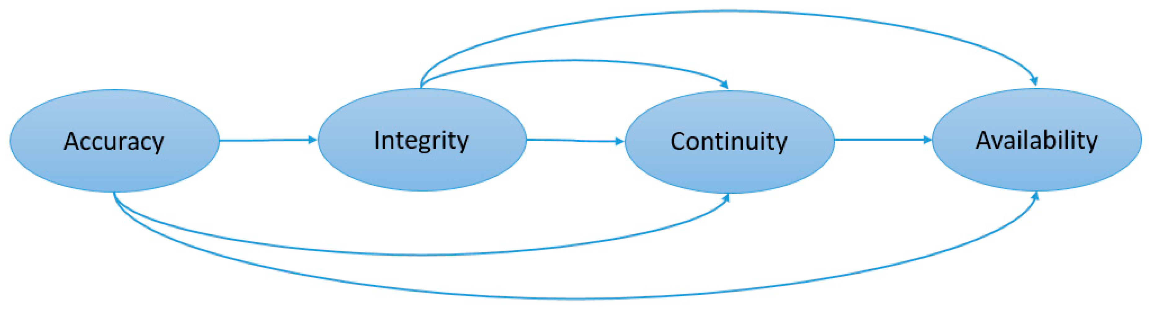
These four criteria are linked to each other by definition, as is shown in
Figure 1. While accuracy is the initial stage within PBN, the trustworthiness of a navigation system is specified based on the confidence level of accuracy as integrity. Continuity is the simultaneous success rate of accuracy and integrity requirements during an intended operation period. Lastly, the navigation system is available only if accuracy, integrity and continuity requirements are fulfilled.
PNT data is the most critical contributor to guidance and control stages, and the Global Navigation Satellite System (GNSS) is one of the primary PNT sources here because of wide coverage, high accuracy, and relatively low cost of the corresponding navigation solutions.
GNSS navigation is able to provide accurate positioning and timing data under the open space conditions for a wide range of applications in both military and civilian domains. Vulnerabilities of the GNSS-based PNT are also well known; it can be affected in both intended (jamming, spoofing, etc.) or unintended (multipath, atmospheric effects, etc.) ways. Many current and future applications of UAV are related to dull, dirty and dangerous (3D) tasks, e.g. work at natural disaster scenes, supporting public safety or routine goods delivery [
3]. In many such cases, the navigation environment will inevitably become GNSS challenging, or even GNSS denied. The 3D applications of UAVs are mostly in urban environments and at the altitudes below building heights [
4]. GNSS performance degrades during low altitude flights in urban areas because of masking and multipath effects from the buildings, structures and vegetation. In order to mitigate the degradation, various alternative PNT solutions are suggested as complementary navigation sources to work with GNSS in cooperation, while others focus on substitutes for GNSS [
5]. Due to increased payload capacity of modern UAVs and better availability of high-quality sensors, multi-sensor navigation is one of the most promising complementary solutions for GNSS-based UAV navigation these days [
6]. Conventionally, fusion of GNSS with Inertial Measurement Unit (IMU) is used for these purposes [
7,
8]. Additional sensors, such as LIDAR, odometer, magnetometer, etc., that can be used for fixing other navigation parameters are utilized for building a more comprehensive and reliable navigation system [
9]. Vision-based methods [
10], such as Simultaneous Localization and Mapping (SLAM) [
11] and ground-based navigation systems [
5] are also considered as alternative PNT sources for navigation in GNSS challenging or denied environments.
While alternative PNT solutions have specific advantages in particular environments and missions, GNSS, however, remains the main navigation source (when it is available) as it provides the best positioning and timing in most of the cases. Hence, monitoring of GNSS performance is one of the critical tasks for future integrated multi-sensor navigation systems, which allows one to estimate and maintain the integrity of GNSS-based navigation and to make appropriate decisions, e.g., concerning required alternative sensors, fusion algorithm parameters or augmentation solutions.
The most common integrity monitoring approaches, which are currently in use are Satellite Autonomous Integrity Monitoring (SAIM), GNSS Integrity Channel (GIC) and Receiver Autonomous Integrity Monitoring (RAIM) [
12], where SAIM focuses only on satellite and orbital errors, GIC takes into account the environmental errors sourced by transmission environment and RAIM monitors receive errors in addition to other errors from satellites and transmission paths. The range and position error models are characterized in open-sky conditions in these integrity monitoring approaches; therefore, integrity monitoring quality is highly degraded in urban environments because of the impact of multipath and satellite obscuration. The following challenges exist for integrity monitoring in urban air mobility applications [
13]:
Integrity monitoring algorithms require a large amount of data for integrity checks, but the amount of available data dramatically decreases in urban environments because of limited satellite visibility.
Assumption of a single fault, which is frequently required for existing integrity monitoring solutions, is no longer valid for urban environments due to multipath and line-of-sight issues.
Integrity measures, once available, could be used in multiple ways, e.g. for sensor switching or performance prediction. For example, authors in [
14] implemented a rule-based sensor switching technique based on the integrity flags generated for each of the considered PNT sources. Another way to use integrity information is presented in [
15] with a performance prediction by a Bayesian network based on the integrity failure rates of error sources.
It is known [
16] that dilution of precision (DOP) coefficients are among the biggest contributors to the positioning accuracy and, therefore, are linked to the integrity of the whole GNSS-based navigation system. Usage of DOP fields in addition to the conventional potential field method is suggested in [
17] as one of the most recent and prospective examples of UAV path planning in known urban areas. Geometric DOP and the number of visible satellites were simulated for two different constellations, GPS and Galileo, and three different cut-off elevations at a specific time and position in [
18]. Work [
19] also provides a distribution of DOP coefficients and the number of visible satellites for GPS, Galileo, GLONASS and BeiDou under two different elevation levels. The satellite visibility and positioning accuracy under different sky view conditions are analyzed in [
20] for GPS and GLONASS. Another work in the Asia–Australia region provides an ambiguity DOP and positioning accuracy analysis combining GPS and Galileo constellations and regional navigation systems, IRNSS and QZSS [
21]. All these works analyze how DOP varies in time when different constellations are considered and under different environmental conditions. However, analysis of the environmental parameters, such as cut-off elevation and satellite visibility, for their joint use for integrity monitoring purposes received little attention in the publications known to authors. Additionally, methods using DOP coefficients or DOP mapping approaches have the following shortcomings for UAV integrity monitoring or path planning applications in urban areas:
In low-cost receivers, DOP coefficients are calculated by applying a matrix inversion to each quad (four-combination) of the visible satellites (although there are some alternative methods) for selecting subsets of satellites with optimal positioning performance [
22]. The DOP update and continuous mapping during the flight in this way are computationally very expensive and not feasible for smaller UAVs. Instead, elevations and number of visible satellites can be extracted from navigation message without any calculation for quick updates.
DOP maps, even in a static environment, are time-varying because of the movement of satellites, so their validity can change during the flight and integrity risks may increase. Due to their time-varying nature, DOP maps are not well suited for the provision of integrity limitations. With using time-independent environmental variables, such as cut-off elevation, integrity risks can be analyzed more accurately before and during the flight.
The use of DOP coefficients for accuracy or availability characterization was thoroughly studied by many authors. Nevertheless, application of DOP maps is mostly limited to availability analysis and does not include integrity requirements. One of the most recent examples of DOP maps generation and application can be seen in [
23], where authors use scanned environment profiles for visibility analysis and DOP prediction for an availability analysis. We use a different approach that can be beneficial when no scanned information was available. Moreover, we focus on integrity analysis, which was not covered previously using either DOP coefficients or elevation and visibility criteria.
Considering the previous works and mentioned challenges, this paper concerns integrity monitoring of the GPS-based UAV positioning in urban environments. We focus on the analysis of environmental parameters to derive limiting values suitable for integrity characterization within an urban air mobility concept. For this purpose, we consider the influence of cut-off elevation and satellite visibility on the behavior of DOP coefficients and, therefore, the integrity of the positioning for UAVs.
One of the key novelties of our integrity monitoring approach is in the proposition and use of DOP-based indirect protection levels as the replacement of the standard position error-based protection levels, as DOP coefficients can be extracted from receiver outputs during flight, unlike unobservable position errors. Another novel proposition is to supplement DOP-based integrity measures with parameters specific to the immediate environment that allow for estimating integrity in a particular environment and can be used to decide on mitigation measures in cases of observed integrity failures.
2. Integrity Monitoring
The purpose of the integrity monitoring is to detect errors and generate timely warnings in case the integrity limits are violated. The integrity criteria defined by ICAO [
24] are:
Horizontal/Vertical Protection Levels (HPL/VPL),
Horizontal/Vertical Alert Limits (HAL/VAL),
Time-to-Alert (TTA), and
Integrity Risk.
VAL/HAL and VPL/HPL represent a vertical distance and a radius of circle in the horizontal plane with center at the true user position, as illustrated in
Figure 2 [
25].
TTA is the maximum allowable time before warnings, and accordingly, integrity risk is the probability of computing a position that is out of defined bounds without warning within the TTA. Alert limits are defined based on the requirements of missions and applications, while protection levels are calculated by users at the receiver level. Simply, protection levels are set statistically as boundaries of the position errors of the particular navigation equipment.
Although there are no commonly accepted regulations for alert limits and TTA for UAV navigation, an initial approximation can be obtained from ICAO’s requirements for Category I approach operations. According to these requirements, vertical guidance (APV-I) is set to 40 m and 50 m for HAL and VAL, respectively; TTA is specified as 10 s, and integrity risk should be less than 1−2 × 10
−7/h. Alert limits defined by the European GNSS Agency for safety-critical applications [
26] are tighter: 5–10 m horizontally and 10–25 m vertically. The environment for urban UAV operations can be characterized based on reasonable assumptions of 30 m street width and 65 m building height, which are common in the US and Europe [
27]. Therefore, in this study, 10 m and 25 m are selected as HAL and VAL limits, respectively, for positioning integrity simulations in urban environments using a generic GPS receiver.
Integrity can be monitored based on analysis of different types of errors. The error sources that affect GNSS performance and their usage in integrity monitoring were discussed in [
28,
29]. RAIM is the simplest way for monitoring navigation performance because it only needs pseudo-range measurements by the receiver. RAIM is not operational with less than five satellites, although the pseudo-range measurements are still available. Additionally, because standard RAIM is able to detect only one fault each time, it is not well suited for working in urban environments, where this assumption is usually not valid. Advanced RAIM (ARAIM), Relative RAIM (R-RAIM) and Extended ARAIM (ERAIM) algorithms are still under development, aiming to improve integrity monitoring and fault detection performance, and the existing issues in urban applications are not solved yet [
30].
SAIM systems specifically focus on satellite-based faults. Its efficiency in detecting orbital errors is much better than both RAIM and GIC. However, its capability to detect user segment errors, which are caused by local environments, stays behind RAIM. Orbital parameter errors are hard to detect at the later stages when they are masked by other error sources, and if they cannot be detected, a persistent error in positioning and timing may occur at the receiver [
31]. Hence, the trustworthiness of the ephemeris message should be checked at the user segment again. The validity check of ephemeris data can be made at the receiver by using Issue of Data Ephemeris (IODE) [
32], which is broadcasted in sub-frames 2 and 3 separately.
Unlike RAIM and SAIM, GIC is an externally supported method; it relies on reference data from control and monitoring stations for integrity analysis. GIC provides a direct and efficient integrity monitoring, but it is a complex and slow technique because of the infrastructural requirements. Its coverage area is also limited by the range of monitoring stations. Satellite-Based Augmentation System (SBAS) and Ground-Based Augmentation System (GBAS) can be mentioned as recent examples of the GIC approach. However, they cannot detect local GNSS errors, such as multipath and obscuration, in urban environments [
33].
Overall, the usage of classical integrity monitoring approaches is challenging in urban environments due to local error sources. Integrity monitoring systems in use have limited availability in urban environments and cannot provide required integrity monitoring performance. Since availability issues of integrity monitoring systems mostly depend on satellite visibility and satellite geometry issues, DOP coefficients, cut-off elevations and number of visible satellites should be investigated in order to improve integrity monitoring performance for local and urban applications.
The Stanford–ESA Integrity Diagram [
34] is one of the useful tools that have been proposed in order to identify and assess integrity risks and integrity failures. This diagram illustrates the integrity risks based on a comparison between position error (PE), protection level (PL) and alert limit (AL). Integrity events are defined through misleading operations, and hazardously operations with respect to the specific areas of the Stanford–ESA Diagram as it is seen in
Figure 3. During normal operations, measurements are expected to appear in the white triangular zone, which represents the nominal operating conditions. Although the Stanford diagram illustrates the integrity risks, TTA should be additionally assessed in order to understand whether a limit exceeding is an integrity failure or not. A time-integrity plot is usually employed in this case; it provides the time history of position errors that can be used to separate integrity failures and sudden changes.
Total receiver positioning error consists of two components: User Equivalent Range Error (UERE) and DOP. The standard deviation of the receiver positioning error
is defined in [
36] as follows:
where
denotes standard deviation of UERE, which is based on estimate of positioning inaccuracy from a single satellite and is calculated for every satellite independently. Typical UERE budget for an L1 frequency C/A code receiver is given in
Table 1 [
36].
The UERE budget estimation is made under ideal satellite geometry condition (DOP = 1). Position error increases with an increase in DOP according to Equation (1). Considering that the impact of UERE elements on the accuracy of the receiver remains approximately the same unless the condition of the transmission line and quality of receiver significantly changes, this study is focused on the analysis of DOP variation and assessment of the most critical environmental parameters, which affect DOP in urban environments and the corresponding positioning integrity.
DOP is presented by non-dimensional measurements (i.e., coefficients) representing the relative positioning of the satellite and receiver to each other in terms of their effect on the positioning solution quality. According to different sort of accuracy metrics, there are seven DOP coefficients. These are Geometric DOP (GDOP), Time DOP (TDOP), Position DOP (PDOP), Horizontal DOP (HDOP), Vertical DOP (VDOP), East DOP (EDOP) and North DOP (NDOP). The relationship between DOP coefficients is presented in Equation (2).
Although there is no common agreement on the terminology describing the quality of navigation performance based on DOP coefficient values, DOP values are characterized in this study with respect to similar works in the literature [
18,
19] and our test results as shown in
Table 2.
DOP coefficients can be calculated as follows:
where
and
are the elevations and azimuths of the best four satellites for DOP calculations.
DOP values multiply positioning error of the receiver and increase with the following anomalies:
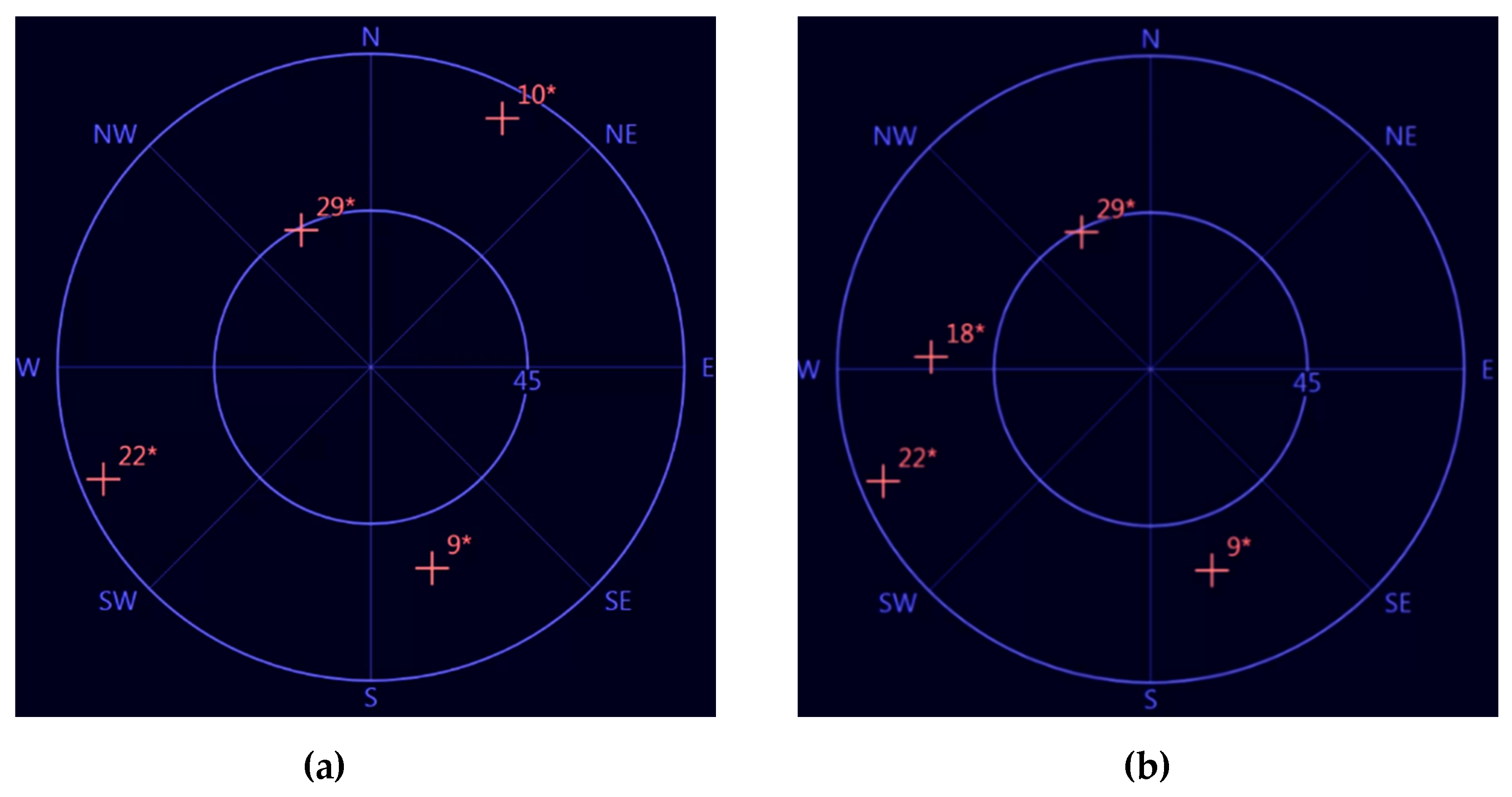
Satellite geometry has a direct impact on DOP coefficients. Even under normal conditions, because of the movement of satellites and vehicle with the antenna installed, geometry is continuously changing based on the number of visible satellites and their positions. Larger DOP values mean worse satellite geometry. The overall quality of satellite geometry also varies according to receiver locations on the Earth. While observations from the equatorial region give a high number of visible satellites and high-quality satellite geometry, a localization near the arctic circle can be very challenging based on satellite visibility and geometry [
37]. Good and bad satellite geometry examples are illustrated in
Figure 4.
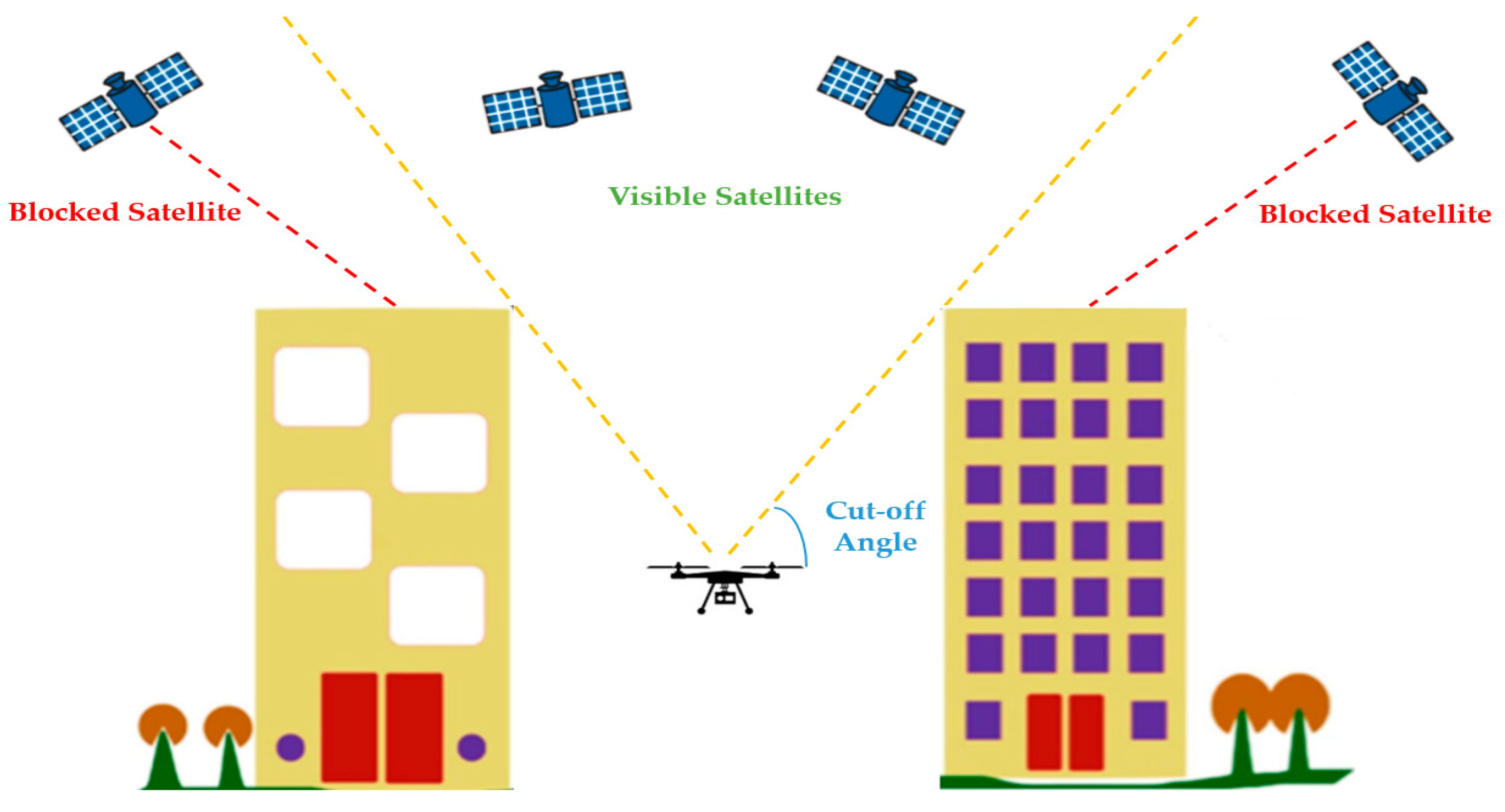
Satellite obscuration is another factor affecting DOP coefficients. In fact, obscuration acts as an elevation cut-off mask and has a direct effect on the number of visible satellites by corrupting user-satellite geometry. As a result, DOP coefficients are increased. Especially in urban environments, because of the high buildings and other obstructions, cut-off elevation may increase significantly. While high cut-off elevation affects satellite visibility, low satellite elevations can also cause multipath, which is beyond the scope of this paper. Thus, specifying the integrity limitations based on cut-off elevation is beneficial for detecting integrity risks caused by local error sources.
In contrast to integrity monitoring systems aimed at aviation applications, such as one described in [
27], urban environment sets different challenges that generally require a different approach for integrity monitoring. Due to smaller sizes of UAVs, the difference in flight pattern in urban areas in comparison to larger aircrafts and the complexity of the environment, one of the main challenges that need to be addressed, is related to integrity failures due to the obscuration pattern, and it can be expressed through the cut-off elevation imposed by the buildings.
Figure 5 illustrates the typical urban environment and the physical impact of cut-off elevation. This challenge defines the focus of our work related to integrity analysis in urban environments through corresponding environmental parameters and observables.
The integrity of the positioning and corresponding accuracy aspects directly depends on the distribution of position error. In general, 95th percentile position error is used to characterize the accuracy of the navigation system and its protection levels. However, integrity risks are defined at the much stricter level with higher percentiles such as 99.99999th in order to make sure the position errors do not exceed specified HAL or VAL boundaries. For this kind of very sensitive estimation, the standard deviation of error distribution is not always sufficient for ensuring the required reliability. Gaussian overbound and sigma inflation methods have already been suggested in the recent researches for correction of Gaussian distribution. While cumulative distribution function (cdf) overbounding for unimodal and symmetric distributions [
38] and paired overbounding [
39] methods are the most common examples, a combined method which involved both methods has been investigated in [
40]. This combined method is applied at the data processing stage of our study for sigma corrections.
3. Simulation
3.1. Simulation Setup
A large amount of data is required to understand the impact of environmental parameters on navigation performance. These data can be simulated, collected by a real receiver, or found from publicly available databases. It should be noted though that isolation of the error sources in the datasets from real scenarios is difficult due to uncertainties of the transmission environment. Moreover, it is challenging to set a local urban environment in a way that addresses our test requirements entirely. Even if it is possible, another challenge occurs at the space segment and transmission environment arrangements since we have no control over them. Thus, a combination of software and hardware simulation devices were selected in this study in order to simulate all segments of the GPS navigation environment instead of experiments in a physical environment, where a real flight test in this sort of GNSS challenging environments under high cut-off elevations will cause high safety risks.
The simulation environment employed in this study for integrity analysis consists of Spirent GNSS Simulator GSS7000 controlled by the SimGen software as outlined in
Figure 6. SimGen [
41] provides a variety of options to define scenarios and parameters related to all GNSS segments. Based on the definitions set in SimGen, GSS7000 generates not only navigation messages but also the navigation environment with all details, such as the position of satellites and receiver, potential faults, tropospheric or ionospheric effects and obstructions. With scenario definitions in the GSS7000 simulator, effects of different error sources in the navigation environment can be separated and studied independently.
At the second step of the simulation environment, a MATLAB-based receiver model was used to obtain position information based on the environment simulated by GSS7000 for the following analysis. When using real receivers for this type of experiment, results may change dramatically from case to case depending on the quality of the receiver and specifics of the implemented algorithms. Therefore, the software receiver has been selected to conduct experiments in order to minimize effects of unknown receiver-based errors, ensure reproducibility of results and allow for future algorithms improvement studies.
In this work, an open source receiver model, goGPS [
41], was used for fundamental receiver calculations. In our tests, inputs and outputs of the model were modified to integrate it with GSS7000 and observe desired navigational parameters. The input data for the receiver model are presented in Radio Technical Commission for Maritime Services (RTCM) format; outputs are DOP coefficients, with receiver position expressed in Latitude–Longitude–Altitude (LLA) and in East–North–Up (ENU) coordinates. For simplicity, the receiver’s initial position was selected as (0,0,0) based on LLA coordinates, and the urban environment was produced in the environment editor of the simulator.
Simulations in this study were conducted based on a single frequency (L1) GPS constellation scenario for a generic urban environment defined through the corresponding elevation map in the simulator. Assuming that the receiver is at the ground level, the cut-off elevation angles in urban areas vary between 20 and 60 degrees. A value of 30° was taken as the maximum value for cut-off elevation during the simulations; beyond this value, the GPS-based navigation is not usable according to preliminary results. The other assumptions made were as follows: UAV is flying a maximum of 10 m below the roof level and in the middle of 30 m wide street with a 30° maximum cut-off elevation.
The flowchart of the proposed approach for analyzing integrity is shown in
Figure 7.
At the first simulation, the reference model of DOP impact on the accuracy was established. Positioning results were acquired and analyzed statistically under 5° cut-off elevation, which represents the open sky condition. Six test constellations with different DOP values, as shown in
Table 3, were defined in the Spirent GSS7000 simulator, and navigation messages were generated for each of them. Since the DOP is affected by variation in the numbers of satellites available to the receiver, test constellations were limited to four visible satellites. Other satellites were disabled for each test to cancel the effect of the number of visible satellites.
Positioning outputs of the selected software receiver were collected for 30 min (approximately 1800 measurements). Probability density function (pdf) and cumulative distribution function (cdf) of the positioning error were produced from these outputs. Thirty-minute simulation provides reliable test data for each case; at the same time, it allows one to prevent dramatic DOP changes and loss of satellite visibility because of the movement of the satellites. The errors were obtained through the comparison of positioning data from the receiver with the ground truth from the simulator. From the analysis of positioning accuracy results, also utilizing the sigma inflation technique for better error representation, the upper DOP limits were specified to reflect alert limits. Then, indirect protection levels are defined as HDOP and VDOP values that are ensuring the integrity risks remain below 1−2 × 10⁻⁷/h.
At the second simulation, the distributions of DOP coefficients and the number of visible satellites were obtained under different cut-off elevations. Simulation for each cut-off elevation was covering a twelve hour period from 12 am to 12 pm on August 30, 2019. The twelve-hour period was intentionally selected for this simulation to match the orbital period of GPS satellites (~11.967 h); this period should give a comprehensive overview of visible satellites’ configurations. Simulated cut-off elevations for this simulation start at 5° and increase by 5° up to 30°. Using these results the limiting values of cut-off elevation and number of visible satellites can be derived based on predefined HDOP and VDOP, which, in turn, correspond to positioning error boundaries obtained from the first simulation. Lastly, indirect protection levels (integrity zones) mapping is produced according to the results of the first and second simulations.
3.2. Simulation Results
During the statistical analysis of the first simulation results, mean values, 67th percentiles, and 95th percentiles of absolute position error of all simulated cases were calculated as presented in
Table 4. As expected, position errors steadily increase with increasing DOP coefficients. Considering assumed alert limits from
Section 2 (10 m horizontally and 25 m vertically) one can see from
Table 4 that position errors are within the alert limits for the first four test cases. More specifically, the 95th percentile of the horizontal error is within alert limits when HDOP ≤ 3.13, and for the vertical error, this is also true when VDOP ≤ 5.13. In cases 5 and 6, navigation based on GPS only cannot be considered safe both horizontally and vertically.
For the purposes of integrity analysis, 95th percentile error cannot provide enough confidence to meet assumed integrity requirements. According to the assumed integrity requirements, the expected rate of position error measurements falling outside of the nominal operation zone in the Stanford–ESA Diagram should not exceed 1−2 × 10⁻⁷/h. Integrity failure occurs when PE > PL > AL during more than TTA, which is specified as 10 s. For generality and reproducibility of the results, achievable HPL and VPL are calculated based on UERE of the employed receiver, which represents the condition where HDOP and VDOP equal 1. In this case, derivation of achievable protection levels for different test configurations is a straightforward task.
Achievable protection levels are calculated from position error and DOP measurements of the first four test cases since PE is higher than AL in the last two cases. For more sensitive analysis, sigma correction following approach [
40] is also applied while obtaining the pdf of the position errors. The 99.99998th percentile of UERE is accepted as a protection level to guarantee that integrity risk is below 1−2 × 10
−7/h.
The alert limits we have specified in
Section 2 are based on assumptions about the urban environment, such as buildings’ heights and street sizes, which may be changed, for instance, for applications with more strict requirements to positioning errors. If this is a case, requirements to acceptable HDOP and VDOP will be tightened. Additionally, since HPL and VPL are specified based on the employed receiver model performance, protection levels can slightly change for another receiver model based on its UERE. Calculated UERE based on Equation (1) and its 95th, 99th and 99.99998th percentile values after sigma correction are presented in
Table 5. Protection levels with various DOP values can be calculated according to Equation (6).
where
is the 99.99998th percentile of UERE.
After specifying base values of HPL and VPL considering HDOP = VDOP = 1, the impact of cut-off elevation on DOP coefficients should be investigated to derive achievable protection levels under various cut-off elevation levels.
Table 6 shows the distribution of DOP coefficients for different cut-off elevation levels. It can be seen that for cut-off elevations up to 5° HDOP is less than 1 with 95.08% probability. Similarly, HDOP is always less than 2 and 3 for cut-off elevations at or below 15° and 20°, respectively. At the 25° level, the probability of HDOP being higher than 5 is approximately 1.6%. Starting from a cut-off elevation of 30°, availability issues begin to appear due to insufficient number of visible satellites.
When analyzing vertical performance, we can see that VDOP coefficients are always less than 2 at 5° cut-off elevation without observable risk and with 3% risk at 10°. VDOP at these cut-off elevations is always less than 3. At 15°, VDOP remains below 5 with no integrity risk. At 20°, while the risk is about 4% for VDOP = 5, VDOP = 7 can be guaranteed. When the cut-off elevation is at or above 25°, vertical positioning availability issues start to be observed.
Using these distributions of HDOP and VDOP, achievable protection levels can be derived following Equation (6) for each cut-off elevation, to be used as indirect integrity measures instead of the corresponding non-observable position errors. The 99.99998th percentiles of HDOP and VDOP distributions for each cut-off elevation are accepted for this purpose.
Calculated horizontal and vertical protection levels with less than 2 × 10
−7/h integrity risk are shown in
Table 7 along with the corresponding DOP-based indirect protection levels. It should be noted that some values were not defined during the simulation. Because of unavailability issues, HPL cannot be defined at 30°, and VPL cannot be defined for 25° and 30° cut off elevations. These cut-off elevations represent essential integrity risks for flights of UAVs with single-mode GPS-based navigation in urban environments.
As a complementary tool for integrity analysis, the time history of HDOP and VDOP coefficients during half-day simulation under different cut-off elevations can be used as shown in
Figure 8. Horizontal dotted lines represent DOP-based indirect protection levels. The figure shows when, for how long and how often these protection levels are exceeded during the simulation period; therefore, a time-to-alert analysis can be conducted based on these graphs.
Below 20° cut-off elevation, both HDOP and VDOP coefficients are measurable for all time without any availability issues. Sharp increases in HDOP and VDOP values are observed above 20° and 25° cut-off elevations, respectively. Specified HPLs are not exceeded below 20° cut-off elevations. However, at 25° cut off elevation, observed horizontal integrity failures are two times longer than the TTA limit: 42 s and 210 s. Besides, vertical integrity failures are observed too: at 15° as a continuous event of duration 672 s and at 20°—continuously over a period of 408 s.
Using results from
Figure 9, the smallest number of visible satellites can be established for each cut-off elevation. It can be seen that at 20° cut-off elevation at least five satellites are visible. At 15° cut-off elevation, this number increases to six. At 10° and 5° cut-off elevations, there are seven and eight visible satellites during the 12 h simulation period, respectively. It can also be seen that the required minimum of four satellites cannot be guaranteed at all times at 25° cut-off elevation. They are only visible for approximately 96% of the simulation time.
Both statistics and time history of DOP results show that cut-off elevation can be used as a parameter during the integrity monitoring due to its complementarity to DOP variation in terms of enhanced knowledge on positioning accuracy. Nevertheless, analysis of cut-off elevation limits may struggle in the differentiation of scenarios with high DOP and issues due to the insufficient number of satellites. So, we need to introduce another parameter to guarantee that the alert limits are not exceeded when cut-off elevation is high. Variation of DOP is not only dependent on cut-off elevation in urban environments but is also directly related to the number of visible satellites. In order to demonstrate this effect, let us consider together
Figure 8, which shows a time history of DOP variation over a 12 h simulation period and
Figure 9, showing how the number of visible satellites changes during the same period of time for each cut-off elevation. It can be seen from these figures that poor satellite visibility causes sharp increases of HDOP and VDOP.
4. Discussion
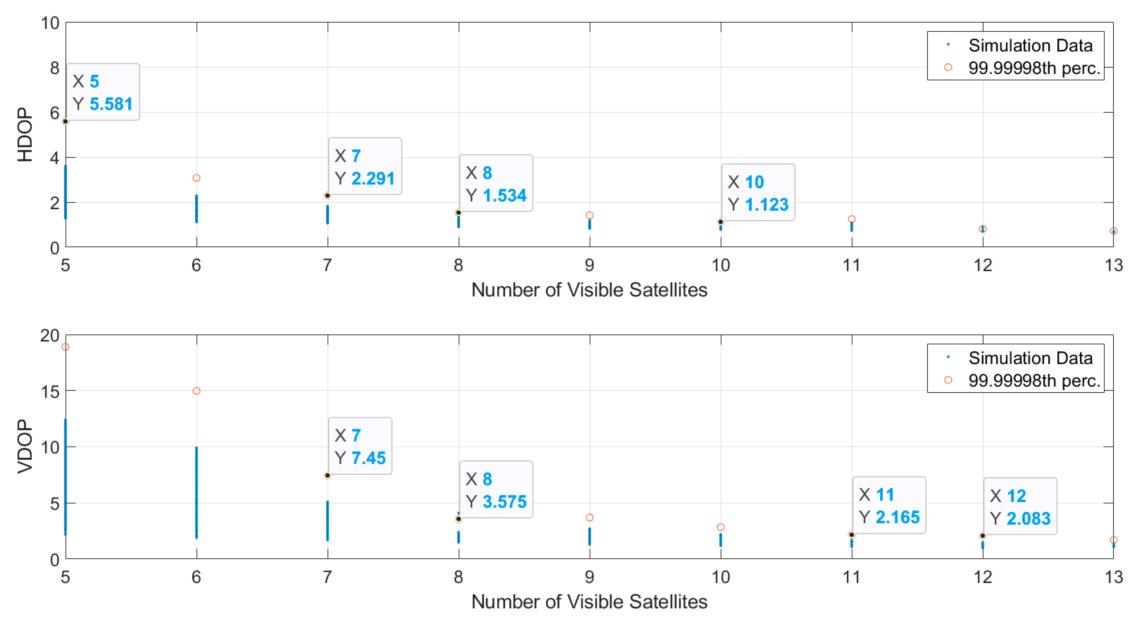
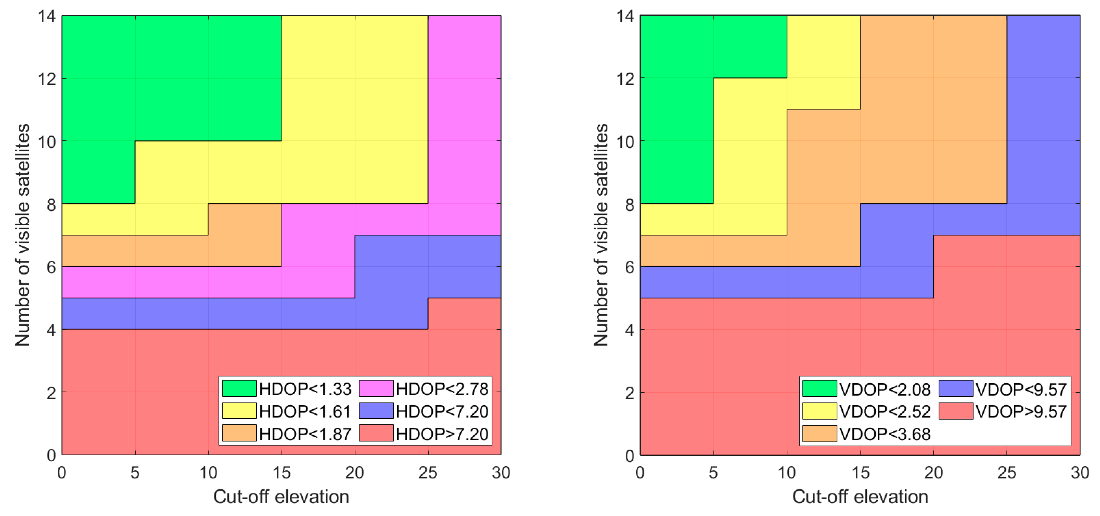
According to the above results, one can see that the number of visible satellites along with the cut-off elevations can be used to characterize integrity based on observed DOP values. In order to derive limiting cut-off elevations based on the acceptable integrity risks, we first explore the relationship between satellite visibility and DOP. For this purpose, 99.99998th percentiles of HDOP and VDOP are calculated from the results of the second simulation for each number of visible satellites, as shown in
Figure 10. In this figure the relationship between DOP and satellite visibility can be analyzed independently from the cut-off elevations. It shows the necessary number of visible satellites that provides the required, for a given integrity, the upper boundary of DOP, which is especially important at high blockage conditions.
For horizontal positioning integrity, at least five visible satellites are required to ensure HDOP < 5.581, seven visible satellites are required to ensure HDOP < 2.291 and eight visible satellites are required to ensure HDOP < 1.534. HDOP below 1.123 can be achieved if at least ten satellites are visible. For vertical positioning integrity, at least seven visible satellites are required to ensure VDOP < 7.45, eight visible satellites are required to ensure VDOP < 3.575, eleven visible satellites are required to ensure VDOP < 2.165 and twelve visible satellites are required to ensure VDOP < 2.083. According to these results, DOP-based indirect protection levels can be specified using cut-off elevation and satellite visibility to describe GPS-based positioning integrity in terms of protection level zones.
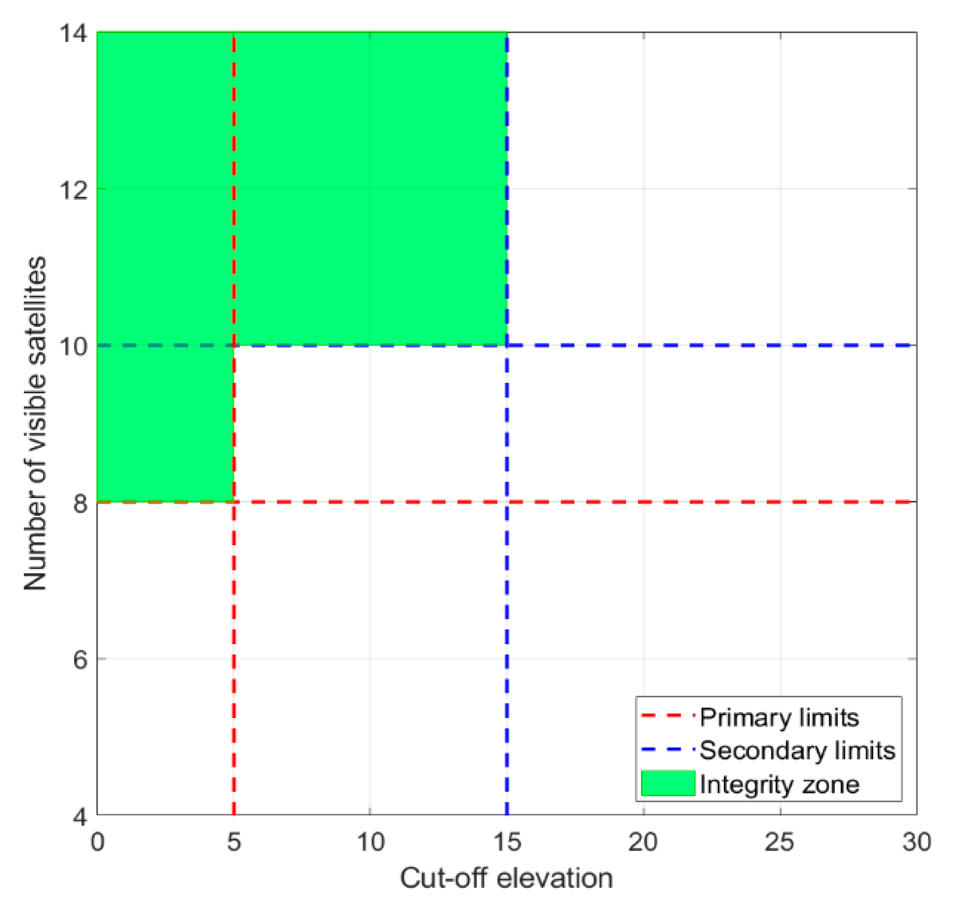
To explain how this can be achieved, let us consider an example of the protection level zone in
Figure 11 expressed in the form of HDOP < 1.3373, which corresponds to
Figure 12. HPL = 7.7973 m and 5° cut-off elevation with regards to
Table 7. The smallest number of visible satellites observed during the simulation corresponding to 5° cut-off elevation is 8, following results shown in
Figure 9. These two parameters define the primary boundaries of the protection level (integrity) zone. Inside each zone, it can be considered that integrity requirements can be guaranteed for specified protection levels.
To define secondary boundaries, the minimum number of visible satellites to guarantee HDOP < 1.3373 is taken from
Figure 10 as 10. According to
Figure 9 and
Figure 10 visible satellites can be observed only up to 15° cut off elevation. Hence, 10 visible satellites and 15° cut-off elevation forms secondary boundaries of the protection level zone. These secondary boundaries are required to cover the cases where cut-off elevation is exceeded, but there are still enough satellites to satisfy integrity requirements.
Finally, the union of these two zones defines the integrity zone based on indirect protection levels considering both cut-off elevation and satellite visibility.
Following this idea, we have compiled results of the second simulation in
Figure 12, which visualizes indirect protection levels (in the form of the limiting DOP values) with respect to cut-off elevations and number of visible satellites.
Considering that the integrity failure condition when HPL > HAL, we specify integrity zones based on HPL = HAL and VPL = VAL. To maintain the required integrity level UAV should stay within these zones during the flight. Assumed in
Section 2 HAL and VAL for the scenario of UAV flight in urban environment (10 and 25 m, respectively) transform into limits of HDOP < 1.87 and VDOP < 3.68 according to our simulation results. From
Figure 12, it follows that UAV should be within green, yellow or orange zones in order to satisfy these requirements. The conditions can be checked using observables obtained from the receiver position solution and environmental parameters. If one of the three arguments (DOP, number of visible satellites and cut-off elevation) are outside of the boundaries, the integrity flag should be raised followed by the predefined mitigation measure.
If the environment is known, the operational altitude of the UAV and the route can be defined before the flight in order to avoid exceeding the alert limits. If this happens anyway, UAV can ascend and decrease cut-off elevation to cope with potential GPS losses. If there is no chance to ascend because of the mission requirements or environment limitations, alternative navigation sensors or systems must be activated to continue flight.
Another point for discussion is how UAV acquires information for this type of integrity monitoring during the flight. Number of visible satellites and satellite elevations can be read from the broadcasted navigation message. As the cut-off elevation is dependent on both the height of buildings and altitude of UAV, it can be either estimated from visible satellite elevations or measured as the angle between UAV and the top of buildings. This can be done using additional sensor data or data extracted from an external source, such as a 3D map. Detection of this angle is out of the scope of this study but is included in the scope of future work.
Suggested protection levels and operational zones will support path and mission planning either before or during the flight. Because of the variation of building heights in urban environments, transitions between the operational zones will be happening during the flight. Considering changes in urban environments, the most critical advantage of our approach against the direct usage of DOP is quick integrity update capabilities at low computational cost.
Another important advantage of our approach is generality and time independency. DOP maps can be generated based on predicted DOP levels for known environments only, e.g., using scanned results. However, these maps are not available if the environment is not known or changed. DOP can also significantly change during the flight because of the movements of satellites; therefore, maps should be accounting for these changes too.
The findings from the analysis of the impact of cut-off elevation and number of visible satellites on DOP coefficients are generic for any kind of urban air mobility application as these results are independent of the receiver model. However, the relationship between DOP and position error is dependent on the employed receiver model. It should be taken into account that equivalent horizontal and vertical position errors for specified DOP levels might change based on the receiver UERE.


