Article

Financial Sustainability Evaluation and Forecasting Using the Markov Chain: The Case of the Wine Business

1
Donbass State Engineering Academy, 84300 Kramatorsk, Ukraine
2
PJSC “Artwinery”, 84500 Bakhmut, Ukraine
3
Maritime Law and Management Faculty, National University “Odessa Maritime Academy”, 65000 Odessa, Ukraine
4
Lithuanian Institute of Agrarian Economics, 03220 Vilnius, Lithuania
*
Author to whom correspondence should be addressed.
Sustainability 2020, 12(15), 6150; https://doi.org/10.3390/su12156150
Submission received: 28 June 2020 / Revised: 19 July 2020 / Accepted: 27 July 2020 / Published: 30 July 2020
(This article belongs to the Special Issue Sustainability Assessment)

Abstract

:
This paper proposes a framework for assessing the financial sustainability of a wine producing company. The probabilistic approach is used to model the expected changes in the financial situation of an enterprise based on the historical trends. The case of an enterprise in Ukraine is considered as an illustration. The Markov chain is adopted for the forecasting exercise. Using the Markov chain framework allows one to predict the probability of financial security change for several periods ahead. The forecast relies on the transition probabilities obtained by exploiting the historical data. The proposed framework is implemented by construction of the financial security level transition matrices for three scenarios (optimistic, baseline and pessimistic). The case study of a Ukrainian wine producing company is considered. The possibilities for applying the proposed method in establishing anti-crisis financial strategy are discussed. The research shows how forecasting the financial security level of a company can serve in anti-crisis financial potential buildup.

1. Introduction

The permanent perturbations in financial markets increase attention to business entities’ solvency in the context of mechanisms ensuring their financial security [1,2,3,4]. The external shocks tolerant business with financial security and without signs of liquidity or solvency losses in the medium and long-term perspectives, determines mesoeconomic (sectoral) stability, which, in turn, serves as one of the prerequisites for sustainable development at the macro level.
The need to study business financial security in the wine sector of Ukraine is highlighted by the fact that its profitability declined in recent years: in 2017, it was only 4.4% as compared to 8.4% in 2011–2012 [5]. Besides, all the wine production distribution in retail turnover was reduced. A special focus should be the significant reduction in the share of domestic wine products, which was not observed in previous periods. Declining sales, financial results and other negative phenomena in the winemaking of Ukraine indicate the growing threat to enterprises of the sector in terms of financial security. The need for research into financial management and sustainable growth is needed to ensure their financial stability. Moreover, the financial analysis should take environmental considerations into account in the further stages [6,7].
Ensuring financial security is possible only through a rational and effective controlling system. Such a system should be able to detect and eliminate deviations from accepted financial security criteria, leveling or avoiding threats and risks of industry development. An effective controlling system allows one for the early detection and prevention of threats for financial sustainability.
The approach proposed in this study allows ensuring financial security at all levels of socio-economic systems. The early detection of threats allows government agencies and business entities to maintain the smooth functioning of the micro level and the corresponding financial stability at the macro level. Thus, ensuring the financial security of the industry is a dynamic process of balancing the financial condition of the branch business entities with state support capabilities (both direct financial and indirect, regulatory and legislative). The prerequisites for the formation of stability, soundness, security and effectiveness of the branch business entities allow to implement the developed macroeconomic security initiatives in the strategic dimension to ensure the long-term economic growth of the country. In this paper, we propose a framework based on the Markov chain that allows using historical data for forecasting the shifts in financial security. We discuss the case of a wine producing enterprise.

2. Literature Review

The theoretical fundamentals of business financial management and financial security have been highlighted in the literature. In particular, A. Baranovskyi [8] and M. Yermoshenko [9] dedicated their work to the formation of theoretical and methodological foundations of financial security, determining its levels and the relationship between them. The studies stress that the macro-level financial security and financial security of companies have close mutual influence. Y. Kartuzov [10], I. Moiseienko and O. Marchenko [11], G. Telnova [12], A. Ursul and T. Ursul [13] and V. Vudvud [14] focused on a systematic approach to the formation of conceptual provisions of financial stability and security of companies. The need to consider all financial aspects in the implementation of policies to counter threats and risks of loss for companies’ financial health was stressed.
Indicators of companies’ financial condition were also discussed. V. Acharya et al. [15] focused on the financial risks associated with increasing corporate debt in emerging economies and emphasize the need for timely regulation of financial risks at the macro level. M. Frank and V. Goyal [16] discussed the factors influencing decision making regarding the capital structure of US firms. S. Carstina et al. [17] considered asset management and their profitability in ensuring financial stability. U. Hamid and A. Won Kie [18] concluded that there is a negative relationship between fund performance and liquidity and a non-linear relationship between them. Nie et al. [19] analyzed the dynamics in the investment costs, O. Kravchenko et al. [20] and R. Khirivskyi et al. [21] pointed out that an effective model of the agri-food and land markets should provide for a systematic development in a stable vector that takes into account the synergistic effect and the internal potential of the economic system. B. Fetai [22] determined that the impact of financial integration depends on the development of internal financial markets, macroeconomic stability and the quality of institutions.
The methodological aspects of ensuring business financial security were explored by E. Altman [23], T. Bogdanova [24], O. Ivashchenko [25], N. Mahas [26], A. Shtanhret et al. [27], Y. Shvets et al. [28], H. Tkachuk [29] and others. E. Altman [23] dedicated his work to the prediction of corporate bankruptcy and the formation of a corresponding economic and mathematical model. T. Bogdanova et al. [24] used the tools of neural networks to evaluate the financial stability. O. Ivashchenko [25] and N. Mahas [26] proposed to conduct rating of the level of financial security of the enterprise. An enterprise financial security assessment based on the identification of the largest external and internal threats is conducted by A. Shtanhret et al. [27]. Indicative methods of estimating and improving the normative values of coefficients, which do not always take into account changes in the external environment of the enterprise and the very specificity of its activity, are investigated by Yu. Shvets et al. [28]. H. Tkachuk [29] proposes a system of indicators for evaluating the effectiveness of management decisions made by a tenant of an integrated property complex and for assessing probable risk. Khomutenko [30] discussed the methodological issues of state finance system analysis.
A great advance in the development of the theoretical foundations of wine industry enterprises management was made by O. Harkusha [31], V. Kucherenko [32], L. Nekrasova and K. Nekrasova [33], M. Popova [34] and Y. Tintulov [35] indicated that due to the presence of serious problems, Ukraine’s wine industry is experiencing a significant economic downturn and requires measures to improve state regulation. Institutional factors were considered as a source of threat for the entrepreneurs of the wine industry by L. Nekrasova and K. Nekrasova [33].
The existing methodological approaches to a comprehensive assessment of business entity financial security are based mainly on the analysis and evaluation of indicators by liquidity, financial stability and profitability groups with their subsequent interpretation according to stability, pre-crisis and crisis conditions and financial security criticality level. The financial security of business entities should be considered in regards to industry-wide trends or specific problems in the financial activities of an individual business entity. Industry-wide reasons are characterized by predictable dynamics of indicators caused by macro- or meso-economic factors and political conditions [36]. Specific reasons cause unpredictable events or unplanned situations at the micro level, which can lead to a decrease in the level of financial security. Such specific reasons are extrinsic for the whole sector. The problems related to management can be tackled at the enterprise level, yet sector-wide issues require the intervention of government agencies [37,38,39].
Turning to studies of the relationship between the financial security of business entities and macro environment factors, D. Bidzhoyan and T. Bogdanova [40] propose the approach to accounting for changes in macroeconomic factors and comparing them with changes in the financial results of an enterprise based on the construction of polynomial functions of the 2nd degree. R. Mamede [41] considers the relationship between financial macroeconomic stability and industrial growth in Italy and Portugal. The author concludes that the development of industry in both countries is largely a consequence of factors that are essentially not related to financial stability, although it has a certain indirect effect on price competitiveness and corporate financial results. In the author’s opinion, the greatest influence on the companies in Italy and Portugal was made by the global financial crisis of 2007–2008 and its economic and financial consequences. S. Nassar [42] investigated the influence of macroeconomic and political factors on the steel industry and related sectors. In particular, the author notes the factor of foreign trade relations in the prospects of the metallurgical industry. Comprehensive evaluation and forecasting of the financial security of the wine business have been addressed in a cursory manner. The financial security of the Ukrainian wine business is further considered in this study.

3. Methods and Data

The preliminary comprehensive evaluation of the wine business’ financial security can be carried out based on the chart method devised by W. Shewhart [43,44]. The basic method has been extended in recent studies [45]. The essence of this tool is the formation of control charts that allow monitoring the level of financial security represented by indicators and identifying types of changes in the process. The changes are assessed according to certain rules, associated with the control value limits. When applying these criteria, the control chart is divided into regions measured in standard deviation. For indicators that should be maximized, these regions are below the average line (arithmetic average for non-standardized indicators of business activity and profitability and standardized values for liquidity and financial stability indicators):
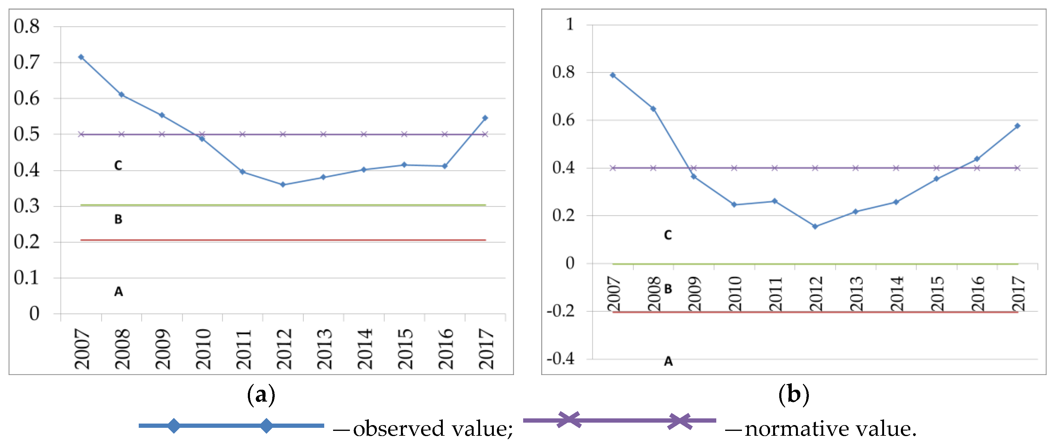
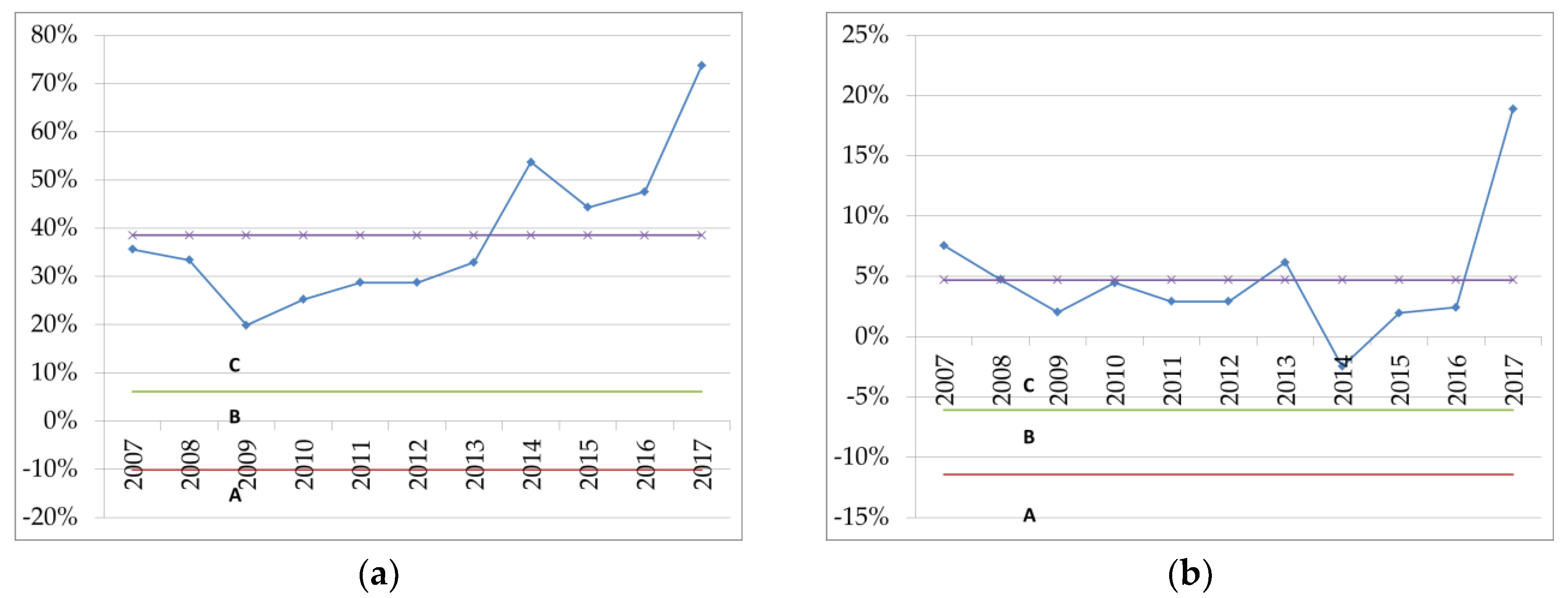
  • C—the region characterizes the unstable state of the indicator,
  • B—the region related to pre-crisis state of the indicator (preventive measures are required),
  • A—characterizes the critical or crisis state of the indicator and requires the use of more radical activities to ensure financial security.
For indicators to be minimized, these regions should be arranged above the average line and have similar interpretation.
A generalization of the financial security evaluation through Shewhart charts relies on the scoring. The rules for scoring are defined as follows: score of 1 is attributed if an observation is on the normative level or above it (respectively on or below it for indicators that should be minimized); score of 0.5 is attributed for points in the region C; score of 0.25 is attributed for observations in region B; zero score is attributed for observations in region A. In this case, for each performance, the integral indicator of financial security takes the following form:
I P k = t = 1 n X k t n
where IPк is the integral performance of financial security according to the k-th indicator; n is the number of periods; Xкt is the k-th indicator value in the period t.
The following indicators are applied: X1 is the net working capital flexibility; X2 is the current (total) liquidity ratio; X3 is the quick ratio; X4 is the absolute liquidity (solvency) ratio; X5 is the financial autonomy ratio; X6 is the current assets to equity ratio; X7 is the capital productivity ratio; X8 is the operating cycle duration; X9 is the financial cycle duration; X10 is the book debts repayment rate; X11 is the owned capital turnover; X12 is the total capital turnover; X13 is the output profitability; X14 is the activity profitability; X15 is the return on assets; X16 is the owned capital profitability. In such a case, indicators X1X4 form a group of liquidity indicators, X5X6 is the group of financial stability indicators, X7X12 is the business activity indicators and X13X16 is the profitability indicators.
The evaluation of financial security level by groups of indicators is carried out as follows:
I G j = k = 1 m I P k m
where IGj is the integrated financial security indicator represented by the j-th group of indicators; m is the the number of indicators in the group. The above-mentioned measure identifies the most groups of indicators and the corresponding management measures.
Another measure determines the level of business financial security by years:
I t = k = 1 f X k t f
where It is the integral indicator of financial security in the t period; f is the number of indicators (in the proposed system it equals 16).
For a qualitative evaluation of the integrated financial security indicators, the verbal-numerical Harrington scale was used (Table 1).
The subject for the proposed approach is a business entity operating in the production of grape wine, namely the public joint-stock company (PJSC) “Artwinery”, located in Bakhmut, Donetsk region. The calculated values of financial security indicators for the company are given in the Table 2.
One can note a rather stable state of the PJSC Artwinery: in 2017, almost all indicators were within appropriate limits and mainly exceeded branch indicators of financial condition, which emphasizes the actual state of financial security. At the same time, the potential for the preventive maintenance of the enterprise financial security, including measures to increase business activity, namely, increasing the turnover of capital and the structure of the assets, will reduce the duration of the operating and financial cycles of the joint-stock company. Shewhart charts were constructed for the liquidity indicators of PJSC Artwinery (Figure 1).
As indicated by the data, three of the four indicators of the enterprise liquidity (net working capital, current liquidity, quick liquidity flexibility) were above the norm during the whole analyzed period. An exception is the absolute liquidity indicator, which was in region C, indicating an unstable state of the indicator. However, at the end of 2017, the indicator corresponds to the normative value.
For the financial stability indicators of PJSC Artwinery, the Shewhart charts take on the form, evident in the Figure 2. We can state a trend towards threats to financial security in 2007–2012. In particular, in 2010–2016 the indicators were in region C, indicating an unstable state of the indicator. However, in 2013–2017, the situation has a positive tendency towards strengthening financial security.
For business activity indicators that do not have an established standard, the middle line is determined on the basis of the arithmetic mean (Figure 3). Most of the indicators until 2014 had a negative trend and in 2014 they became closer to sector B, i.e., the pre-crisis state. However, this situation cannot be called critical, because according to the Shewhart’s methodology, the tendency becomes apparent during five or six observer points.
We present a graphical analysis of the profitability indicators by Shewhart charts in Figure 4. The center line on these charts is the arithmetic mean of the indicators. According to the charts, profitability management is the most stable during 2007–2013, where observer points deviate slightly from the center line.
In general, the financial security of PJSC Artwinery is at the sufficient level. Further forecasting of financial security will be carried out using the Markov chains [46,47]. The Markov chain essentially consists of many transitions, which are determined by probability distribution. Such probabilities are determined by observing the transitions from one state to another. The probability distribution of transitions is presented as a transition matrix of the Markov chain.
To study business financial security in the wine sector using the example of PJSC Artwinery, we define five possible states of financial security: very high level of financial security (s1); high level of financial security (s2); medium level of financial security (s3); low (pre-crisis) level of financial security (s4); crisis (critical) level of financial security (s5). Thus, the transition matrix has a 5 × 5 order with each element indicating the probability of transition from state si to state sj. Moreover, the elements in each row of the matrix should add up to unity as each row represents a probability distribution.
To formalize the proposed strategy, it is necessary to determine the transition probability from si to sj state during three paths: h1—increase of the financial security level; h2—stable financial security level; h3—decrease of the financial and economic security level. We will address the possible paths through the meso- and macro-economic conditions for the wine sector.

4. Results

The research addresses the three major issues: (i) the dynamics in the financial security indicators and the overall situation; (ii) transition among the financial security levels; (iii) projection of the future financial security levels based on the transition probabilities. The Markov Chain approach is adopted to operationalize the proposed model and generate conclusions regarding the expected financial state of the company. By using the financial security indicators for PJSC Artwinery and the Shewhart chart, the score table is formed (Table 3). Based on the trends in the Ukrainian and global economy, one can define the three meso- and macro-economic states relevant to the case of the PJSC Artwinery:
  • recovery periods: 2010, 2015;
  • periods of stability: 2007, 2011, 2012, 2013, 2016, 2017;
  • downturn periods: 2008, 2009, 2014.
Based on the data in Table 3, we determine the number of transitions from one level to another (increase or decrease or stationary level):
in the recovery periods (2 periods), the number of periods with increasing financial safety indicators is 1 (thus, P ( h 1 | a 1 ) = 1 / 2 ); the number of periods with stable level of the indicators is 1 ( P ( h 2 | a 1 ) = 1 / 2 );
in the stability periods (6 periods), the number of business financial safety decreases is 1; the stationary level is 5;
in the downturn periods (3 periods), the number of business financial safety decreases is 2; the stationary level is 1.
The data in Table 3 provide the basis for calculating conditional probabilities in three scenarios: optimistic, baseline and pessimistic. The probability for transition from s i to s j is under scenario r = { o , b , p } is denoted as P i r ( s j ) .
For the optimistic scenario, there are only recovery and stability periods with equal probability (0.5). These probabilities are denoted as P o ( a 1 ) and P p ( a 1 ) . Indeed, they do not change across i . At s 1 , the transition to a higher level of financial security is impossible (it is assumed that a 1 implies staying at s 1 in this case). The probability of staying in s 1 is determined as follows:
P 1 o ( h 1 | a 1 ) = 0.5 ;   P 1 o ( h 2 | a 1 ) = 0.5 ;   P 1 o ( h 1 | a 2 ) = 0 ;   P 1 o ( h 2 | a 2 ) = 5 / 6 = 0.83 ;
P 1 o ( s 1 ) = P 1 o ( h 1 | a 1 ) P o ( a 1 ) + P 1 o ( h 2 | a 1 ) P o ( a 1 ) + P 1 o ( h 1 | a 2 ) P o ( a 2 ) + P 1 o ( h 2 | a 2 ) P o ( a 2 ) = 0.5 0.5 + 0.5 0.5 + 0 0.5 + 0.83 0.5 = 0.92.
Respectively, the probability of transition to a lower level of financial security will be:
P 1 o ( s 2 ) = 1 P 1 o ( s 1 ) = 0.08.
To calculate the probability to transit from financial security level s2 to level s1 (i.e., to improve financial security), the pre-set probability of increase in the financial security h1 and probability a1 for the meso- and macro-economic conditions of the sector functioning are multiplied:
P 2 o ( h 1 | a 1 ) = 0.5 ;
P 2 o ( s 1 ) = P 2 o ( h 1 | a 1 ) P o ( a 1 ) = 0.5 0.5 = 0.25.
Staying at level s2 will occur both in case of the increasing (a1 = 0.5) and stable (a2 = 0.5) level of the meso- and macro-economic conditions of the sector functioning:
P 2 o ( h 2 | a 1 ) = 0.5 ;   P 2 o ( h 2 | a 2 ) = 5 / 6 = 0.83 ;
P 2 o ( s 2 ) = P 2 o ( h 2 | a 1 ) P o ( a 1 ) + P 2 o ( h 2 | a 2 ) P o ( a 1 ) = 0.5 0.5 + 0.83 0.5 = 0.67.
Respectively, the transition probability from level s2 to level s3 is obtained residually as:
P 2 o ( s 3 ) = 1 P 2 o ( s s ) P 2 o ( s 2 ) = 0.08.
The probability of transition from level s2 to levels s4 and s5 is zero as such cases are not observed during the training process.
The procedure outlined above can be applied to obtain probabilities for financial security levels s3s4:
P 3 o ( s 1 ) = 0 ;   P 3 o ( s 2 ) = 0.25 ;   P 3 o ( s 3 ) = 0.67 ;
P 3 o ( s 4 ) = 0.08 ;   P 3 o ( s 5 ) = 0 ;   P 4 o ( s 1 ) = 0 ;
P 4 o ( s 2 ) = 0 ;   P 4 o ( s 3 ) = 0.25 ;   P 4 o ( s 4 ) = 0.67 ;
P 4 o ( s 5 ) = 0.08 .
When transiting from level s5, it is only possible to consider the probability of a rise to the financial security level s4, which is equal to 0.25. In other cases, the probability of staying in level s5 in crisis is 0.75. Thus, we obtain a probability matrix of the transition among the financial security levels for the PJSC Artwinery taking into account the meso- and macro-economic conditions and the internal financial management possibilities. The transition matrix for the optimistic scenario takes the following form:
M o = ( 0.92 0.08 0 0 0 0.25 0.67 0.08 0 0 0 0.25 0.67 0.08 0 0 0 0.25 0.67 0.08 0 0 0 0.25 0.75 ) .
For the baseline scenario, the probability of rise and stability periods is 0.4 (i.e., P b ( a 1 ) = 0.4 and P b ( a 2 ) = 0.4 ) and the financial security decrease probability is 0.2 ( P b ( a 3 ) = 0.2 ). The transition matrix for the baseline scenario is obtained following the same procedure as outlined for the optimistic scenario. However, the probabilities of the economic conditions are different and the resulting transition matrix is as follows:
M b = ( 0.8 0.2 0 0 0 0.2 0.6 0.2 0 0 0 0.2 0.6 0.2 0 0 0 0.2 0.6 0.2 0 0 0 0.2 0.8 ) .
For the pessimistic scenario, there are only stability periods with the probability 0.5 and the decrease periods with the same probability. Therefore, P p ( a 2 ) = 0.5 and P p ( a 3 ) = 0.5 . We obtain the transition probability matrix for PJSC Artwinery financial security level depending on the meso- and macro-economic conditions and the internal financial management following the procedure outlined below:
M p = ( 0.58 0.42 0 0 0 0 0.58 0.42 0 0 0 0 0.58 0.42 0 0 0 0 0.58 0.42 0 0 0 0 1 ) .
The obtained transition matrices define the probabilities for switching among the financial security levels. Note that we used the three scenarios when defining these matrices. The resulting transition matrices can be applied to predict the future level of financial security in n years. In our case, we control for data up to year 2017 (Table 3). Therefore, the forecasts are available for year 2017 + n. First, we define the probabilities of switching from the very high financial security level ( s 1 ) considering 2017 as the reference point. The following row vector directs the forecast:
M ( 0 ) = ( 1 0 0 0 0 ) .
Then, the forecast horizon n determines the degree the transition matrix is raised up to. The latter matrix is then multiplied by the direction vector M ( 0 ) . Therefore, the transition probabilities for s 1 during time period n (after year 2017) and scenario r are defined as follows:
M r ( n ) = M ( 0 ) ( M r ) n = M r ( n 1 ) M r , r = { o , b , p } , n = 1 , 2 ,
Let us consider the projections up to 2020 for the optimistic scenario. Hence, we pick n = 1 , 2 , 3 and r = o . For 2018, the probability of the business financial security level change is calculated as:
M o ( 1 ) = M ( 0 ) ( M o ) 1 M r ( n 1 ) M r = ( 1 0 0 0 0 ) ( 0.92 0.08 0 0 0 0.25 0.67 0.08 0 0 0 0.25 0.67 0.08 0 0 0 0.25 0.67 0.08 0 0 0 0.25 0.75 ) = ( 0.92 0.08 0 0 0 ) .
Similarly, projections for year 2019 are obtained by setting n = 2 :
M o ( 2 ) = M ( 0 ) ( M o ) 2 = M o ( 1 ) M o = ( 0.92 0.08 0 0 0 ) ( 0.92 0.08 0 0 0 0.25 0.67 0.08 0 0 0 0.25 0.67 0.08 0 0 0 0.25 0.67 0.08 0 0 0 0.25 0.75 ) = ( 0.87 0.13 0 0 0 ) .
Finally, the forecasts for 2020 under the optimistic scenario are derived as
M o ( 3 ) = M ( 0 ) ( M o ) 3 = = M o ( 2 ) M o = ( 0.87 0.13 0 0 0 ) ( 0.92 0.08 0 0 0 0.25 0.67 0.08 0 0 0 0.25 0.67 0.08 0 0 0 0.25 0.67 0.08 0 0 0 0.25 0.75 ) = ( 0.83 0.16 0.01 0 0 ) .
Similar calculations are applied for the baseline and pessimistic scenarios. In the case of the baseline scenario, the transition probabilities for 2020 are obtained as
M b ( 3 ) = M ( 0 ) ( M b ) 3 = ( 0.6 0.31 0.08 0.01 0 ) .
For the pessimistic scenario, one has
M p ( 3 ) = M ( 0 ) ( M p ) 3 = ( 0.2 0.43 0.30 0.07 0 ) .
Obviously, the optimistic scenario foresees possible transition to s 3 , whereas transition towards s 4 is possible under the baseline and pessimistic scenarios (besides s 1 and s 2 ). The results for expected change in the financial security levels for each year are further summarized in the scenario-wise manner.
The analysis based on the Markov chains revealed that, according to the optimistic scenario, when there is no economic turbulence and no adverse conditions for the wine sector development, PJSC Artwinery is likely to keep a high level of financial security up until 2021. The probability of decrease to the high level of financial security in 2020 is only 16%. The decrease to the medium level of financial security is even less likely with probability of only 1% (Figure 5).
The baseline scenario assumes an increase in the operating conditions of the sector with the 40% probability, the stable state with the 40% probability and economic contraction with the 20% probability. In this instance, the probability of deteriorating operation conditions and errors in internal management are more likely. Therefore, the probability of remaining at the very high level of financial security in 2020 is 60%, whereas the decrease to the high level is associated with probability of 31% (Figure 6). The probability for falling down to the medium level of financial security is 8%, whereas the probability for approaching the pre-crisis level is 1%. Obviously, the probability of the latter two financial security states is small. However, they still require attention in regards to the financial stability capacity building within a company.
The pessimistic scenario assumed either the stability or the decline of the sector. The resulting probability of maintaining a very high financial security level in 2020 is much lower (0.20) if contrasted to the other two scenarios (Figure 7). The highest probability corresponds to a decrease in financial security to the high level (0.43). A decrease in financial security to the medium level is possible with probability of 30%. Finally, the probability of the pre-critical situation is 7% (for 2020).
The above-mentioned information gives grounds for the financial security capacity building. The appropriate level of financial security will increase the adaptability of business entities to external unfavorable conditions and may improve management internally. This study applied data from PJSC Artwinery to measure its financial security level and demonstrated the forecasting possibilities that allow for anti-crisis financial capacity building within the enterprise. Preventive anti-crisis measures, which include identifying opportunities and hidden reserves to strengthen financial stability, will ensure a high level of financial security and sustainable development of the business entity.

5. Conclusions

This paper applied the Markov chain approach to forecast the financial stability level of a wine producing company. The different scenarios representing possible changes in the economic environment were defined. The multiple financial indicators were taken into account to identify the different states of organizational performance and of financial security. Along with the predefined scenarios (i.e., changes in the states of financial performance and the corresponding probabilities), the transitions among the states of financial security were assessed. The assumed scenarios are related to meso and macroe-conomic conditions relevant to the wine production sector. The results indicated that the anti-crisis financial capacity of the enterprise is an important issue that can be handled via the analysis of the prospective developments in the financial security. In our case, the pessimistic scenario implying stability or decline in the economic environment indicated that transition to lower levels of financial security was imminent. However, the case of the medium or low level of financial security appeared to be less probable. Therefore, the company should re-consider the possibilities for improving its financial performance and revisit the probabilistic forecasts of the financial security level.
The results of the analysis and the proposed model can be applied in sustainability analysis at different levels of management. The impacts of sustainability policies on the financial indicators can be estimated. Then, the proposed method can be applied to ascertain the possible effects of changes in financial indicators on the overall financial security level in the probabilistic setting.

Author Contributions

Conceptualization, N.R.; data curation, H.T.; formal analysis, O.K.; methodology, I.G.; resources, T.B. and D.S.; writing—original draft, N.R. and H.T.; writing—review and editing, O.K., I.G., T.B. and D.S. All authors have read and agreed to the published version of the manuscript.

Funding

This research received no external funding.

Conflicts of Interest

The authors declare no conflict of interest.

References

  1. Becerra-Vicario, R.; Alaminos, D.; Aranda, E.; Fernández-Gámez, M.A. Deep Recurrent Convolutional Neural Network for Bankruptcy Prediction: A Case of the Restaurant Industry. Sustainability 2020, 12, 5180. [Google Scholar] [CrossRef]
  2. Coppola, A.; Scardera, A.; Amato, M.; Verneau, F. Income Levels and Farm Economic Viability in Italian Farms: An Analysis of FADN Data. Sustainability 2020, 12, 4898. [Google Scholar] [CrossRef]
  3. Guo, A.; Wei, H.; Zhong, F.; Liu, S.; Huang, C. Enterprise Sustainability: Economic Policy Uncertainty, Enterprise Investment, and Profitability. Sustainability 2020, 12, 3735. [Google Scholar] [CrossRef]
  4. Rioux, B.; Galkin, P.; Wu, K. An economic analysis of China’s domestic crude oil supply policies. Chin. J. Popul. Resour. Environ. 2019, 17, 217–228. [Google Scholar] [CrossRef] [Green Version]
  5. State Statistics Service of Ukraine. Available online: http://www.ukrstat.gov.ua/ (accessed on 5 March 2020).
  6. Song, M.; Fisher, R.; Kwoh, Y. Technological challenges of green innovation and sustainable resource management with large scale data. Technol. Forecast. Soc. Chang. 2019, 144, 361–368. [Google Scholar] [CrossRef]
  7. Afum, E.; Osei-Ahenkan, V.Y.; Agyabeng-Mensah, Y.; Owusu, J.A.; Kusi, L.Y.; Ankomah, J. Green manufacturing practices and sustainable performance among Ghanaian manufacturing SMEs: The explanatory link of green supply chain integration. Manag. Environ. Qual. Int. J. 2020. [Google Scholar] [CrossRef]
  8. Baranovskyi, О.І. Financial Security in Ukraine (Assessment Methodology and Support Mechanisms); Kyiv National University of Trade and Economics (KNUTE): Kyiv, Ukrainе, 2004. (In Ukrainian) [Google Scholar]
  9. Yermoshenko, M.M. State Financial Security: National Interests, Real Threats, Security Strategy; Kyiv National University of Trade and Economics (KNUTE): Kyiv, Ukrainе, 2001. (In Ukrainian) [Google Scholar]
  10. Kartuzov, Y.P. Definition of the enterprise financial security: Concept, content, value and functional aspects. Top. Issues Econ. 2012, 8, 172–181. (In Ukrainian) [Google Scholar]
  11. Moiseienko, I.P.; Marchenko, O.M. Management of the Enterprise Financial and Economic Security; Lviv State University of Internal Affairs (LvDUVS): Lviv, Ukrainе, 2011. (In Ukrainian) [Google Scholar]
  12. Telnova, G.V. General positions of the integrated corporative structure financial management concepts determination. Econ. Ann. XXI 2013, 3, 57–60. (In Ukrainian) [Google Scholar]
  13. Ursul, A.; Ursul, T. Environmental Education for Sustainable Development. Future Hum. Image 2018, 9, 115–125. [Google Scholar] [CrossRef]
  14. Vudvud, V.V. Financial security of the enterprise in the conditions of economic instability. Young Sci. 2015, 10, 98–102. (In Ukrainian) [Google Scholar]
  15. Acharya, V.; Cecchetti, S.G.; De Gregorio, J.; Kalemli-Özcan, Ș.; Lane, P.R.L.; Panizza, U. Corporate Debt in Emerging Economies: A Threat to Financial Stability? Brookings Institution, Committee for International Policy Reform: Washington, DC, USA, 2015; Available online: http://www.brookings.edu/research/papers/2015/09/corporate-debt-emerging-economies (accessed on 15 March 2020).
  16. Frank, M.Z.; Goyal, V.K. Capital Structure Decisions: Which Factors Are Reliably Important? Financ. Manag. 2009, 38, 1–37. [Google Scholar] [CrossRef] [Green Version]
  17. Carstina, S.; Siminica, M.; Circiumaru, D.; Tanasie, A. Correlation Analysis of the Indicators of Asset Management and Profitability. Int. J. Econ. Bus. Adm. 2015, 3, 3–21. [Google Scholar] [CrossRef]
  18. Hamid, U.; Won Kie, A. Further Test on Stock Liquidity Risk with a Relative Measure. Int. J. Econ. Bus. Adm. 2016, 4, 56–69. [Google Scholar]
  19. Nie, P.-Y.; Wang, C.; Chen, Y.-H.; Yang, Y.-C. Effects of switching costs on innovative investment. Technol. Econ. Dev. Econ. 2018, 24, 933–949. [Google Scholar] [CrossRef]
  20. Kravchenko, O.; Kucher, A.; Hełdak, M.; Kucher, L.; Wysmułek, J. Socio-Economic Transformations in Ukraine towards the Sustainable Development of Agriculture. Sustainability 2020, 12, 5441. [Google Scholar] [CrossRef]
  21. Khirivskyi, R.; Cherevko, H.; Yatsiv, I.; Pasichnyk, T.; Petryshyn, L.; Kucher, L. Assessment and Analysis of Sustainability of the Socio-Economic Development of Amalgamated Territorial Communities of the Region. Eur. J. Sustain. Dev. 2020, 9, 569. [Google Scholar] [CrossRef]
  22. Fetai, B. Financial Integration and Financial Development: Does Financial Integration Matter? Eur. Res. Stud. J. 2015, 18, 97–106. [Google Scholar] [CrossRef] [Green Version]
  23. Altman, E.I. Financial Ratios, Discriminant Analysis and the Prediction of Corporate Bankruptcy. J. Financ. 1968, 23, 589–609. [Google Scholar] [CrossRef]
  24. Bogdanova, T.K.; Shevgunov, T.Y.; Uvarova, O.M. Application of neural networks for solvency prediction for Russian companies of manufacturing industries. Bus. Inform. 2013, 2, 40–48. (In Russian) [Google Scholar]
  25. Ivashchenko, O.V. The theoretical fundamentals for assessing the level of enterprise financial security. Bull. Zaporizhzhya Nat. Univ. Econ. Sci. 2016, 1, 148–155. (In Ukrainian) [Google Scholar]
  26. Mahas, N.V. Rating estimation of financial security of enterprises. Effic. Econ. 2015, 5. Available online: http://www.economy.nayka.com.ua/?op=1&z=4090 (accessed on 15 March 2020). (In Ukrainian).
  27. Shtanhret, A.M.; Kotliarevskyi, Y.V.; Melnykov, O.V. Financial security of the enterprise: Methodological fundamentals of management. Financ. Ukr. 2013, 11, 56–65. (In Ukrainian) [Google Scholar]
  28. Shvets, Y.O.; Tsykalo, K.S. A methodological approach to assessing the level of industrial enterprises financial security. Sci. Bull. Int. Humanit. Univ. Ser. Econ. Manag. 2017, 25, 162–168. (In Ukrainian) [Google Scholar]
  29. Tkachuk, H.O. Financial security of the enterprise: Assessment of management effectiveness and risk assessment. Econ. Food Ind. 2013, 1, 62–64. (In Ukrainian) [Google Scholar]
  30. Khomutenko, A. Specific Methodological Approaches to Managing State Finances. Montenegrin J. Econ. 2018, 14, 73–82. [Google Scholar] [CrossRef]
  31. Harkusha, O.M. Formation of Effective Winery-Winemaking Subcomplex of AIC of Ukraine: Monograph; National Anti-Corruption Bureau (MDAA): Mykolaiv, Ukrainе, 2001. (In Ukrainian) [Google Scholar]
  32. Kucherenko, V.M. Trends in export-import activities of the wine industry. Econ. Strategy Prospects Dev. Trade Serv. 2015, 2, 279–292. (In Ukrainian) [Google Scholar]
  33. Nekrasova, L.A.; Nekrasova, K.I. Analysis and prospects of development of winemaking enterprises in Ukraine. Black Sea Econ. Stud. 2016, 6, 83–87. (In Ukrainian) [Google Scholar]
  34. Popova, M.M. State regulation of the development of the viticulture and wine industry in Ukraine: Current status, problems and directions of improvement. Econ. Financ. Right 2013, 10, 4–8. (In Ukrainian) [Google Scholar]
  35. Tintulov, Y.V. Improvement of the public administration system of the viticulture and wine subcomplex of Ukraine as a guarantee of its sustainable development. Econ. Innov. 2014, 58, 326–332. (In Ukrainian) [Google Scholar]
  36. Lavrysh, Y. Implementation of Transformative Sustainability Learning into Engineering Curricular. Future Hum. Image 2018, 9, 63–73. [Google Scholar] [CrossRef]
  37. Heldak, M.; Kucher, A.; Stacherzak, A.; Kucher, L. Structural Transformations in Agriculture in Poland and Ukraine: Towards Economic Sustainability. J. Environ. Manag. Tour. 2019, 9, 1827–1841. [Google Scholar] [CrossRef]
  38. Ma, B. Value Shaping of “Ecological Man”: External Standard and Internal Idea. Future Hum. Image 2020, 13, 57–65. [Google Scholar] [CrossRef]
  39. Kim, Y.; Choi, S.; Yi, M.Y. Applying Comparable Sales Method to the Automated Estimation of Real Estate Prices. Sustainability 2020, 12, 5679. [Google Scholar] [CrossRef]
  40. Bidzhoyan, D.; Bogdanova, T. Modelling the financial stability of an enterprise taking into account macroeconomic indicators. Bus. Inform. 2016, 37, 30–37. [Google Scholar] [CrossRef]
  41. Mamede, R.P. Financial (In)Stability and Industrial Growth: The Cases of Italy and Portugal; University Institute of Lisbon: Lisbon, Portugal, 2014. [Google Scholar] [CrossRef] [Green Version]
  42. Nassar, S. Financial Outlook of the United States Steel Industry and Its Role in the Economy Moving Forward. iBusiness 2019, 11, 51–56. [Google Scholar] [CrossRef] [Green Version]
  43. Shewhart, W.A. Economic Control of Quality of Manufactured Product; Van Nostrand: New York, NY, USA, 1931. [Google Scholar]
  44. Shewhart, W.A. Statistical Method from the Viewpoint of Quality Control; The Graduate School, The Deptartment of Agriculture: Washington, DC, USA, 1939. [Google Scholar]
  45. Faraz, A.; Saniga, E.; Montgomery, U. Percentile-based control chart design with an application to Shewhart X and S 2 control charts. Qual. Reliab. Eng. Int. 2018, 35, 116–126. [Google Scholar] [CrossRef] [Green Version]
  46. Markov, A.A. Propagation of the law of large numbers into quantities that depend on each other. Proc. Physics Math. Soc. Kazan Univ. 1906, 15, 135–156. (In Russian) [Google Scholar]
  47. Awwad, M. Influences of Frege’s Predicate Logic on Some Computational Models. Future Hum. Image 2018, 9, 5–19. [Google Scholar] [CrossRef]
Figure 1. Shewhart charts for liquidity indicators of PJSC Artwinery. (a) Dynamics in X1; (b) Dynamics in X2; (c) Dynamics in X3; (d) Dynamics in X4.
Sustainability 12 06150 g001
Figure 2. Shewhart charts for the financial stability indicators of PJSC Artwinery. (a) Dynamics X5; (b) Dynamics in X6.
Sustainability 12 06150 g002
Figure 3. Shewhart charts for business activity indicators of PJSC Artwinery. (a) Dynamics in X7; (b) Dynamics in X8; (c) Dynamics in X9; (d) Dynamics in X10; (e) Dynamics in X11; (f) Dynamics in X12.
Sustainability 12 06150 g003
Figure 4. Shewhart charts for profitability indicators of PJSC Artwinery. (a) Dynamics in X13; (b) Dynamics in X14; (c) Dynamics X15; (d) Dynamics in X16.
Sustainability 12 06150 g004aSustainability 12 06150 g004b
Figure 5. Probability of change of financial security level of PJSC Artwinery according to the optimistic scenario.
Sustainability 12 06150 g005
Figure 6. Probability of change of financial security level of PJSC Artwinery according to the baseline scenario.
Sustainability 12 06150 g006
Figure 7. Probability of change of financial security level of PJSC Artwinery according to the pessimistic scenario.
Sustainability 12 06150 g007
Table 1. Qualitative evaluation of the integrated financial security indicators.
Informal Description of GraduationsNumerical Value
Very high financial security level0.8–1.0
Sufficient financial security level0.64–0.8
Medium financial security level0.37–0.64
Low (pre-crisis) financial security level 0.2–0.37
Crisis (critical) financial security level0.0–0.2
Table 2. Financial security indicators of PJSC “Artwinery”.
Indicator20072008200920102011201220132014201520162017
X10.670.500.310.190.150.080.120.150.200.230.41
X23.162.081.541.251.171.091.131.171.251.301.69
X33.131.991.521.221.151.071.091.061.141.221.46
X40.030.070.020.020.010.010.050.110.100.090.22
X50.720.610.550.490.400.360.380.400.420.410.55
X60.790.650.360.250.260.160.220.260.350.440.58
X7-4.382.701.982.222.142.192.242.421.642.59
X8-359.66343.16270.22340.45392.01423.28427.83756.42510.34525.26
X9-293.83278.03156.89149.81168.86191.90235.77473.85305.85315.84
X10-0.300.350.330.410.450.520.410.560.610.55
X11-1.471.481.781.811.931.781.681.021.431.24
X12-0.970.860.920.790.730.660.660.420.590.59
X1326.10%35.59%33.37%19.85%25.19%28.70%28.70%32.89%53.70%44.28%47.53%
X147.08%7.57%4.75%2.03%4.47%2.91%2.91%6.17%−2.46%1.95%2.42%
X155.82%5.90%3.40%1.46%2.85%1.92%1.94%4.22%−1.01%1.17%2.97%
X168.87%10.19%6.57%3.35%7.57%5.17%4.97%10.33%−2.43%2.46%5.44%
Table 3. Integrated evaluation of PJSC Artwinery based on the financial security indicators.
Indicator20072008200920102011201220132014201520162017IPкIGj
X1111110.5111110.950.88
X2111111111111.00
X3111111111111.00
X40.50.50.50.50.50.50.50.50.50.510.55
X51110.50.50.50.50.50.50.510.680.68
X6110.50.50.50.50.50.50.5110.68
X7 11110.50.50.50.50.50.50.700.76
X8 1111110.250.50.50.50.78
X9 1111110.50.50.50.50.80
X10 111110.50.510.50.50.80
X11 1111110.50.50.50.50.80
X12 11110.50.50.50.50.50.50.70
X130.50.50.50.50.50.50.511110.680.70
X14110.510.50.510.50.50.510.73
X15110.50.50.50.510.50.50.510.68
X16110.510.50.510.50.50.510.73
It0.900.940.810.840.780.690.780.610.660.660.810.77

