Non-Invasive Risk Stratification of Hypertension: A Systematic Comparison of Machine Learning Algorithms

Abstract

One of the most important physiological parameters of the cardiovascular circulatory system is Blood Pressure. Several diseases are related to long-term abnormal blood pressure, i.e., hypertension; therefore, the early detection and assessment of this condition are crucial. The identification of hypertension, and, even more the evaluation of its risk stratification, by using wearable monitoring devices are now more realistic thanks to the advancements in Internet of Things, the improvements of digital sensors that are becoming more and more miniaturized, and the development of new signal processing and machine learning algorithms. In this scenario, a suitable biomedical signal is represented by the PhotoPlethysmoGraphy (PPG) signal. It can be acquired by using a simple, cheap, and wearable device, and can be used to evaluate several aspects of the cardiovascular system, e.g., the detection of abnormal heart rate, respiration rate, blood pressure, oxygen saturation, and so on. In this paper, we take into account the Cuff-Less Blood Pressure Estimation Data Set that contains, among others, PPG signals coming from a set of subjects, as well as the Blood Pressure values of the latter that is the hypertension level. Our aim is to investigate whether or not machine learning methods applied to these PPG signals can provide better results for the non-invasive classification and evaluation of subjects’ hypertension levels. To this aim, we have availed ourselves of a wide set of machine learning algorithms, based on different learning mechanisms, and have compared their results in terms of the effectiveness of the classification obtained.

1. Introduction

Cardiovascular diseases (CVDs) have been increasing worldwide, and their related mortality rate has overtaken that of cancer, making CVDs the leading cause of death in humans. Additionally, CVDs strongly impact healthcare in terms of consuming resources and finances due to the fact that they require long-term monitoring, therapies, and treatment, thus becoming a global challenge.

Since long ago, hypertension has represented one of the most important risk factors for CVDs [1]. For the prediction of the occurrence of acute and chronic CVDs, Blood Pressure (BP) is considered a significant biomedical parameter [2].

Currently, the sphygmomanometer [3] is the most common instrument to measure BP, even if it is considered an invasive sensor. This technique of measurement has been widely recognized and popularized over the last century of development, and it has played a major role in the control of CVDs. However, this sensor is considered invasive because it requires a cuff and a pressure to the forearm when BP is measured. In this way, the measurement can easily be affected by the operation and use conditions, such as the operation of the cuff, and the sitting posture.

Additionally, when the BP is measured in a medical setting, the “white coat phenomenon” could occur, so called because it may happen that the BP values are higher when monitored in a medical setting with respect to when they are measured at home [4]. Therefore, also to avoid this latter problem, new cuff-less screening and CVDs monitoring technologies are very appreciated to control the health status of people and detect patients’ hypertension at home [5].

In this regard, the PhotoPlethysmoGraphy (PPG) is very promising because it is a non–invasive, low-cost, and well–established diagnostic tool [6]. The pulse oximeter, which is the most common PPG sensor, is based on an optical technique that can measure oxygen saturation and heart rate, and it is able to provide general information about the operation mode of the cardiovascular system as well.

In recent years, several approaches based on features extracted from the PPG signal have been proposed in the literature to predict BP or to evaluate hypertension. Some examples of these methodologies are based on the pulse wave velocity [7], or on the pulse transit time [8]. Some others, instead, use particular time-domain characteristics [9], or PPG intensity ratio [10].

A detailed literature review on the recent use of Machine Learning techniques to estimate blood pressure values through the PPG signal is reported in Section 2.

However, none of the mentioned papers reports an exhaustive overview of machine learning methods for the non-invasive classification and evaluation of subjects’ hypertension levels.

In this paper, we wish to overcome this strong limitation of the literature. To this aim, we avail ourselves of a wide set of machine learning algorithms, based on different learning mechanisms, and compare their results in terms of the effectiveness of the classification obtained.

As a conclusion of the study, we expect to have a comprehensive view of the performance of the machine learning algorithms over this specific problem and to find the most suitable classifier.

Additionally, as a further contribution of this paper, we investigate the behavior of the classification algorithms also in terms of risk stratification. This means we consider the discrimination ability provided by an algorithm at different levels of granularity into which the data set can be divided, as reported in, e.g., refs. [4,11,12]. This analysis allows us to ascertain which is the best machine learning algorithm.

The tests have been performed on a new data set built starting from the Cuff-Less Blood Pressure Estimation Data Set [13], freely available on UC Irvine Machine Learning Repository at (www.https://archive.ics.uci.edu). Due to the numerosity of the items and to the different dimensions of the classes of the data set used in this study, the results are reported in terms of F-score, in addition to accuracy, sensitivity, specificity, and precision.

The paper is organized as follows: Section 2 discusses related works. Meanwhile, Section 3 details the building of the data set. Section 4 describes the experiments conducted and the statistical measurements used to assess the quality of the classification performed by each algorithm tested. Finally, the results for both classification and stratification risk are discussed in Section 5.1 and Section 5.2, respectively. Finally, conclusions are provided in Section 6.

2. Related Work

The use of photoplethysmography to estimate blood pressure values by means of Machine Learning techniques is not new in the scientific literature, yet this paper is, to the best of our knowledge, the one in which the highest number of Machine Learning algorithms is considered to fulfill this task. In the following, we report on some of the most recent papers dealing with this issue.

An interesting and recent review of papers dealing with the problem of accurate and continuous BP measuring through the use of mobile or wearable sensors is addressed in ref. [14] by Elgendi and colleagues. It turns out that photoplethysmography is a good solution, as PPG technology is nowadays widely available, inexpensive, and integrable with ease in portable devices. Their conclusion is that, although the technology is not yet fully mature, in the near future, mobile and wearable devices will be able to provide accurate, continuous BP measurements.

One of the first papers dealing with this issue is probably [15], where Kurylyak and colleagues make use of Artificial Neural Networks (ANNs) to find the relation between PPG and BP. The Multiparameter Intelligent Monitoring in Intensive Care waveform database is used to train the ANNs. A number of heartbeats higher than 15,000 is analyzed, and, from each such heartbeat, the values of 21 parameters are extracted. These latter constitute the input to the ANNs. The accuracy values achieved are better than those provided by linear regression.

Another pioneering paper is ref. [16], where Choudhury and colleagues describe a methodology for the estimation of Blood Pressure (BP) through PPG. Their idea is based on two steps. In the first such step, PPG features are mapped with some person–specific intermediate latent parameters. In the second step, instead, BP values are derived from these intermediate parameters. From a model viewpoint, their approach takes into account the 2–Element Windkessel model for the estimation of the total peripheral resistance and arterial compliance of a person by means of PPG features. After this, linear regression is used to simulate arterial blood pressure. A hospital data set is used to carry out the experiments, and the numerical results show absolute errors equal to 0.78 ± 13.1 mmHg and 0.59 ± 10.23 mmHg for systolic and diastolic BP values, respectively. An interesting outcome is that this two–step methodology obtains better results than the direct estimation of BP values from PPG signals.

In ref. [17], Solà and colleagues report on the use of a physiology-based pulse wave analysis algorithm to optical data coming from a fingertip pulse oximeter. They conclude that this algorithm is able to estimate with good accuracy blood pressure changes in-between cuff readings. They suggest that the combined use of their approach and of the standard utilization of oscillometric cuffs can provide increased safety for patients as this can provide non–invasive beat-to-beat hemodynamic measurements.

In ref. [11], Liang and his colleagues consider deep learning to classify and evaluate hypertension starting from PPG signals. Their deep learning scheme relies on continuous wavelet transform and a GoogleNet convolutional neural network. The data they work on consists of a set of 121 recordings from the Multiparameter Intelligent Monitoring in Intensive Care (MIMIC) Database, each of which contains PPG signals and arterial blood pressure ones. They consider the risk stratification problem; hence, they face three different classification tasks: normotensive vs. pre-hypertensive, normotensive vs. hypertensive, and normotensive plus pre-hypertensive vs. hypertensive. The related values for the F-scores have resulted in being equal to 80.52%, 92.55%, and 82.95%, respectively. A finding of this research is that deep learning has allowed obtaining better results than those provided by the classical signal processing endowed with a feature extraction method.

In ref. [18], Rundo and colleagues present an approach for the accurate estimation of both systolic and diastolic blood pressure thanks to the sampling of PPG signals. Their approach does not need any calibration phase. The processing of the PPG signals takes place through an ad hoc bio-inspired mathematical model that relies on the combination of two Machine Learning algorithms, namely a Multi–Layer Perceptron artificial neural network trained with the Back–Propagation algorithm modified as per the Polak–Ribiere approach and an advanced modified version of the Self-Organizing Map (SOM). The resulting accuracy is equal to about 97%, which is better than the performance of a cuff-based sensor for blood pressure measurement.

In ref. [19], Lin and colleagues aim to increase BP estimation accuracy. To this aim, they extract from PPG recordings a set of new indicators and utilize a linear regression method to obtain models for BP estimation. These models rely on the PPG indicators and pulse transit time (PTT). These models are evaluated on the PPG data coming from 22 subjects on which BP fluctuations are induced by means of both mental arithmetic stress and Valsalva’s manoeuvre tasks. The findings reveal that the best estimation model shows a reduction of 0.31 ± 0.08 mmHg in systolic BP (SBP) and 0.33 ± 0.01 mmHg in diastolic BP (DBP) on estimation errors when compared to other methods relying on the use of PPG. Moreover, the best estimation model taking into account both PPG and PPT shows a reduction of 0.81 ± 0.95 mmHg in SBP and 0.75 ± 0.54 mmHg in DBP when compared to other methods based on PPT.

In ref. [4], Liang and colleagues focus on the early screening of hypertension through the use of PPG features. Namely, both a wide set of PPG features and their derivative waves are considered. The features to be used are chosen in six different methods. The authors claim they have been able to find an intrinsic relation between systolic blood pressure and PPG features. Then, several classification algorithms are utilized, i.e., linear discriminant analysis (LDA), cubic SVM, weighted KNN, and logistic regression (LR). Finally, a risk stratification analysis is affected in terms of the F1 score parameter, which shows scores for the normotension versus pre–hypertension, normotension and pre–hypertension versus hypertension, and normotension versus hypertension trials equal to 72.97%, 81.82%, and 92.31%, respectively.

In ref. [20], Radha and colleagues focus on the problem of estimating the nocturnal systolic blood pressure (SBP) dip taking place at night starting from 24-h blood pressure data. This problem is faced by them through the use of a PPG sensor and a deep neural network. The study has enrolled 106 healthy subjects that have been asked to wear a wrist PPG sensor for seven months. From each PPG waveform, HRV features have been extracted. Then, long- and short-term memory (LSTM) networks, dense networks, random forests, and linear regression models have been used to track the trends in BP and to estimate the SBP dips. Deep LSTM networks have turned out to be the most suitable Machine Learning tool for this task.

In ref. [12], Tjahjadi and Ramli propose a method to classify BP by means of the K-nearest neighbors (KNN) algorithm based on PPG. The data are related to 121 subjects, who are divided into normotensive, pre-hypertensive, and hypertensive. The PPG data are not manually preprocessed. The results show values for the F1 score equal to 100%, 100%, and 90.80%, respectively. These values turn out to be better than those obtained by other Machine Learning methods as convolutional neural networks (deep learning), bagged tree, logistic regression, and AdaBoost tree.

As for our own previous work, we started in ref. [21] by using for the first time in the literature Genetic Programming in this field. The aim is to perform regression so as to find an explicit relationship between Electrocardiography (ECG) and Heart Related Variability (HRV) parameters, plethysmography (PPG), and blood pressure (BP) values. The results prove that GP has found suitable explicit mathematical models expressing nonlinear relationships through which both systolic and diastolic blood pressure values can be computed starting from those of ECG, HRV, and PPG. The approximation error has turned out to be lower than two mmHg for both systolic and diastolic BP values.

More recently, in ref. [22], we propose an approach only requiring a PPG sensor and a mobile/desktop device to estimate blood pressure values of subjects in a continuous, real-time, and noninvasive way. The proposal is based on the use of Genetic Programming for the automatic achievement of an explicit relationship expressing blood pressure values as a function of PPG ones. A set of 11 subjects has been used, and the obtained results have been contrasted against those from other regression methods. The numerical results show the superiority of the approach proposed, with root-mean-square error values equal to 8.49 and 6.66 for the systolic and the diastolic blood pressure values, respectively. These are higher than those in our previous paper, yet are still acceptable for international standards, and allow us to design an easy-to-use wearable real–time monitoring system.

3. The Data Set

The data set used in the presented study has been built starting from the Cuff-Less Blood Pressure Estimation Data Set [13], freely available on UC Irvine Machine Learning Repository at (www.https://archive.ics.uci.edu), one of the most used data sets of the scientific literature of this research field.

This latter data set has been created starting from the Multi-parameter Intelligent Monitoring in an Intensive Care (MIMIC) II online waveform database [23] provided by PhysioNet organization. Physiological data were collected by using several patient sensors connected to a Component Monitoring System Intellivue MP-70 (Philips Healthcare). Each monitoring system acquired and digitized multi-parameter physiological data, and processed the signals to derive time series (trends) of clinical measures, such as heart rate, blood pressure, oxygen saturation, etc.

MIMIC II is a reliable database in which the values have been collected in a proper way. It contains a large number of items, so it is well suited for machine learning and deep learning studies.

The Cuff-Less Blood Pressure Estimation Data Set consists of a cell array of matrices, precisely four matrices of 3000 cells for a total of 12,000 instances that corresponds to 12,000 patients.

In each matrix, each row corresponds to one biomedical signal:

• the PPG signal from the fingertip,
• the ABP signal that is the invasive arterial blood pressure (mmHg),
• and the ECG signal from channel II.

All signals have been taken with a frequency of 125 Hz.

Starting from this data set, a new one is created. All processing steps have been performed by using MATLAB, version R2019b, distributed by Mathworks [24].

In our study, we use only the first two signals, which are the PPG signal and the ABP signal.

Precisely, for each subject, the ABP signal and PPG signal are divided into segments with a length of five seconds. On each ABP signal segment, its peaks are found by using the MATLAB findpeaks function. Then, the values of systolic blood pressure (SBP) at the times that correspond to the peaks of ABP signal are considered, and their average is computed.

By using this SBP average, the classification of the segment is carried out. On the basis of both the European [25] and the US [26] guidelines for hypertension management and control, each class has been defined as below:

• Normotension: was defined as SBP < 120 mmHg;
• Pre-hypertension: was defined by SBP of 120 to 139 mmHg;
• Hypertension at Stage 1: was defined by SBP of 140 to 159 mmHg;
• Hypertension at Stage 2: was defined as SBP ≥ 160 mmHg.

Following this procedure, for each patient, we have obtained a number of different items that depends on the total length of the signal. Each of these items is constituted as below:

$$item=id;{\left.\overrightarrow{SamplesPPG}\right|}_1^{625};class$$

(1)

where:

• $id$: is a value that unequivocally identifies each patient;
• ${\left.\overrightarrow{SamplesPPG}\right|}_1^{625}$: is a vector containing the 625 samples of the PPG signal;
• $class$: is the class.

The length of the vector $\overrightarrow{SamplesPPG}$ is 625 because we considered segments of five seconds of a signal sampled at 125 Hz.

As a result of all the processing phase and of the procedure faced, the data set used in this study consists in 526,906 items, 353,840 of which related to class 0 (normotension), 116,879 to class 1 (pre–hypertension), 42,957 to class 2 (hypertension at Stage 1), and 13,230 to class 3 (hypertension at Stage 2). Hence, it is very unbalanced.

As specified before, the original Cuff-Less Blood Pressure Estimation Data Set consists of four matrices, so we have decided to use the first matrix for the training, and the other three for the testing. A detailed subdivision of the items is reported in Table 1.

Table 1. Description of the data set used in this study.

Set	Normotension	Pre-Hypertension	h. Stage 1	h. Stage 2
Training	83,845	27,956	14,092	4810
Testing	269,995	88,923	28,865	8420
Total	353,840	116,879	42,957	13,230

4. The Experiments

4.1. The Algorithms

To run our experiments over the data sets described in the previous Section 3, we have availed ourselves of the Waikato Environment for Knowledge Analysis (WEKA) [27] tool, version 3.8.1. Namely, we have run as many as possible of the therein contained classification tools. These latter are categorised into different groups, in a way that all tools in a given group are based on the same idea that is specific to that group. To give some examples, a first group is based on Bayesian concepts, a second on functions, a third on rules, a fourth on trees, and so on. For each such category, we have focused our attention on some of the therein contained algorithms, namely on those that are often considered the best-performing ones. Therefore, from Bayesian methods, we have taken into consideration the Bayes Net (BN) and the Naïve Bayes (NB). From among the function–based ones, we have chosen Logistic (Log), Multi–Layer Perceptron Neural Network (MLP), Radial Basis Function (RBF), the Support Vector Machine (SVM), and the Weightless RAM-Based Neural Model (Wisard). From among the Lazy methods, we have considered the Instance-Based Learned (K-Nearest Neighbour) (iBk). From the Meta methods, we have used the AdaBoost (AB) and the Bagging (Bag). From among the Rule-based methods, we have chosen the One Rule (OneR), the Repeated Incremental Pruning (JRip), the Partial Decision Tree (PART), and the Ripple–Down Rule (Ridor). Finally, among the tree–based, we have considered the C4.5 decision tree (J48), the Random Forest (RF), and the REPTree (RT).

Table 2 shows the algorithms investigated here. Namely, the first column reports the class of the algorithm, the second the name, the third the acronym used in this paper for it, and the fourth a literature reference for further information.

Table 2. The algorithms used here for the classification.

Class	Algorithm	Acronym	Reference
Bayes:	Bayes Net	BN	[28]
	Naive Bayes	NB	[29]
Functions:	Logistic	Log	[30]
	MultiLayer Perceptron	MLP	[31]
	Radial Basis Function	RBF	[32]
	Support Vector Machine	SVM	[33]
	Weightless RAM-Based Neural Model	Wisard	[34]
Lazy:	Instance-Based Learner (K-Nearest Neighbour)	IBk	[35]
Meta:	AdaBoost	AB	[36]
	Bagging	Bag	[37]
Rules:	One Rule	OneR	[38]
	Repeated Incremental Pruning (JRip)	JRip	[39]
	Partial Decision Tree (PART)	PART	[40]
	Ripple-Down Rule	Ridor	[41]
Trees:	C4.5 decision tree (J48)	J48	[42]
	Random Forest	RF	[43]
	REPTree	RT	[44]

An important issue when running classification algorithms lies in finding a good set for the values of its parameters. We have decided here to run each algorithm with all of its parameters set to the default values that are contained in WEKA. This is because a preliminary phase aiming at tuning the parameter values, and this for each of the here accounted algorithms, would have required an enormous amount of time. This is true in general, and a fortiori holds true here, due to the very large size of the data sets.

As regards the execution times, we have decided to run each algorithm over each data set for one week on a powerful machine endowed with an Intel(R) Xeon(R) CPU E5-2630 v4, 2.2 GHz. If an algorithm has not provided the result within one week, we have decided to report it here as Not Terminated (NT).

4.2. The Statistical Measures

To assess the quality of the classification performed on a data set, several statistical measures are used. They were originally defined for classification in two-class data sets, yet their definition can be easily extended to the classification in sets with a number of classes higher than two as it is the case here.

Let’s start with the definitions for a two-class data set with a total number of items to be classified equal to, say, N. In this case, if we consider one of the two classes as the positive one (e.g., subjects suffering from a given disease) and the other as the negative one (healthy subjects), we have that, after the classification phase has been affected, the data set items are assigned to four different groups:

• true positive: the items belonging to the positive class that are correctly assigned to the positive class, be their number tp;
• true negative: the items belonging to the negative class that are correctly assigned to the negative class, be their number tn;
• false positive: the items belonging to the negative class that are incorrectly assigned to the positive class, be their number fp;
• false negative: the items belonging to the positive class that are incorrectly assigned to the negative class, be their number fn.

The sum of the cardinalities of all these four groups is equal to N.

Starting from these groups, we can define a set of statistical measures, of which we use in this paper the ones described below:

• accuracy $A_c=\frac{tp+tn}{N}$
• precision $P_r=\frac{tp}{tp+fp}$
• sensitivity (or recall) $S_e=\frac{tp}{tp+fn}$
• specificity $S_p=\frac{tn}{tn+fp}$
• F score $F_s=2·\frac{\mathrm{precision}·\mathrm{recall}}{\mathrm{precision}+\mathrm{recall}}$

Each of these indicators considers a different aspect of how the classification has worked. For example, sensitivity and specificity are very commonly used in the medical domain. The specificity is related to the type-I errors, i.e., the negative items that are incorrectly assigned to the positive class. The sensitivity, instead, is related to the type-II errors, i.e., the positive items that are incorrectly assigned to the negative class. Actually, type II errors are more serious: in fact, for binary medical data sets, they represent the ill subjects than are erroneously considered as healthy, which may have fatal consequences. Type-I errors, instead, represent healthy subjects that are erroneously considered as ill, which may generate trouble for the subjects yet is not a fatal situation. F score, instead, is the harmonic mean of precision and recall.

Starting from these definitions in the binary classification domain, these measures prove useful for more classes too. In this case, we compute the values of the parameters for the generic i-th class by considering it as the positive class and contrasting it against all the other classes seen as a unique negative class. Once this is done, the value for each of the measures defined above is computed as the weighted average of the values obtained for each of the classes in the data set, where the weight for a class is the percentage of items belonging to that class.

The values of all these indicators can vary within [0.0–1.0]; the higher the value, the better the classification.

Two important issues should be underlined here.

The former issue is that what usually happens is that when a classification achieves high value for specificity, then the value for specificity is very likely to be low, and vice versa. Hence, a kind of a trade-off is often desirable.

The latter issue is that the accuracy, which is the most widely used parameter, is not a good indicator whenever a data set is divided into classes that are very differently populated, i.e., for unbalanced data sets. This is exactly the case for our data set here, where the two classes related to hypertension contain much lower items that those representing both healthy and pre–hypertension cases. In fact, when using accuracy, it is often the case that an algorithm might achieve high accuracy values, yet, when examining how the data set items have been assigned to the different classes, we can see that all of them have been classified as belonging to the more populated classes, or even to the most populated one. Actually, this takes place for our data set too. Figure 1 shows a clear example of this.

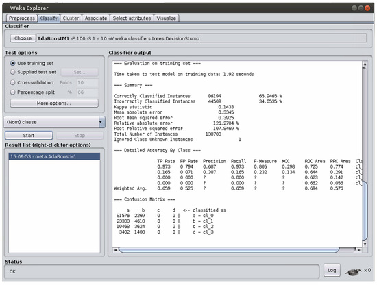
Figure 1. An example of a classification error when the classes are unbalanced.

In this case, the confusion matrix reported in the bottom part of the figure reveals that all the items of the two less populated classes, i.e., those related to hypertension, are assigned to the two classes representing the healthy items and the pre-hypertension ones. This could not be noticed if we considered the accuracy value only. However, this error becomes clearly visible when we look at the F score value, which is now represented as a question mark. Hence, in situations like this one, the most effective index is represented by the F score.

5. Results and Discussion

5.1. Results about the Classification

Table 3 shows the results obtained by each algorithm over the training set and the testing set in terms of the five parameters defined above. The best result obtained over each parameter is reported in bold.

Table 3. The results of the algorithms.

Algorithm	Training					Testing
	${\mathit{A}}_{\mathit{c}}$	${\mathit{P}}_{\mathit{r}}$	${\mathit{S}}_{\mathit{e}}$	${\mathit{S}}_{\mathit{p}}$	${\mathit{F}}_{\mathit{s}}$	${\mathit{A}}_{\mathit{c}}$	${\mathit{P}}_{\mathit{r}}$	${\mathit{S}}_{\mathit{e}}$	${\mathit{S}}_{\mathit{p}}$	${\mathit{F}}_{\mathit{s}}$
BN	67.206%	0.728	0.672	0.751	0.692	67.206%	0.728	0.672	0.751	0.692
NB	34.461%	0.503	0.345	0.485	0.394	73.187%	0.755	0.732	0.778	0.740
Log	72.623%	0.696	0.726	0.645	0.699	77.198%	0.747	0.772	0.662	0.754
MLP	84.957%	0.844	0.850	0.809	0.842	77.517%	0.751	0.775	0.624	0.752
RBF	76.188%	?	0.762	0.753	0.742	79.469%	?	0.795	0.695	0.775
SVM	NT	NT	NT	NT	NT	NT	NT	NT	NT	NT
Wisard	87.211%	0.874	0.872	0.805	0.863	76.658%	0.741	0.767	0.624	0.746
IBk	100.000%	1.000	1.000	1.000	1.000	74.784%	0.737	0.748	0.671	0.741
AB	65.946%	?	0.659	0.412	0.566	69.634%	?	0.696	0.376	0.610
Bag	93.611%	0.935	0.936	0.938	0.935	79.996%	0.781	0.800	0.694	0.785
J48	97.920%	0.979	0.979	0.984	0.979	75.434%	0.743	0.754	0.683	0.748
JRip	78.881%	0.773	0.789	0.704	0.771	76.061%	0.729	0.761	0.580	0.732
RF	100.000%	1.000	1.000	1.000	1.000	80.877%	0.790	0.809	0.704	0.794
RT	84.823%	0.844	0.848	0.861	0.845	77.070%	0.751	0.771	0.668	0.757
OneR	68.152%	0.633	0.682	0.485	0.624	68.775%	0.610	0.688	0.391	0.617
PART	96.016%	0.961	0.960	0.941	0.959	76.131%	0.742	0.761	0.645	0.746
Ridor	79.260%	0.792	0.793	0.716	0.767	74.083%	0.711	0.741	0.513	0.691

As a preliminary note, whenever the question mark “?” is reported in the tables, this means that the problem described in Figure 1 took place, so that a correct computation of the corresponding parameter could not be carried out. NT, instead, means that the run did not end before the one-week timeout set.

If we take into account the results obtained over the train set, we can see that both IBk and Random Forest perform perfectly, as they both achieve the highest value on any parameter considered here.

When, instead, the test set containing previously unseen items is considered, the results show that Random Forest is the algorithm with the best performance in terms of four parameters, i.e., accuracy $A_c$, precision $P_r$, sensitivity $S_e$, and F-score $F_s$. Naive Bayes, instead, has the best performance in terms of specificity $S_p$.

These results obtained by IBk, excellent over training set and lower performance over the testing set, imply that, for this classification task, IBk suffers from overfitting. With this term, we mean that IBk has learned too much from the train set items, while not understanding the general mechanisms underlying this data set to be used for new, previously unseen items as those contained in the test set.

On the contrary, the results for Naive Bayes, quite bad over the training set and much better over the testing set, reveal that this algorithm does not suffer from overfitting for this classification task. Rather, it has been able to understand the mechanisms underlying the data set, as can be proven by its $S_p$ value over the previously unseen items of the data set, which is the highest from among those of all the algorithms considered here.

In conclusion, the use of Random Forest is preferable when facing this data set.

Once it is seen that Random Forest is the best-performing algorithm, we wish to closely examine its behavior over this data set. Table 4 shows the confusion matrix for Random Forest over the Training set, whereas Table 5 contains the same information with reference to the Testing Set. For the sake of space, we have represented in the tables the classes with numbers: NT stands for normotension, PT for pre-hypertension, HT1 for hypertension at stage 1, and HT2 for hypertension at stage 2.

Table 4. The confusion matrix for Random Forest over the Training Set.

Actual Class	Real Class
	NT	PT	HT1	HT2
NT	83,845	0	0	0
PT	0	27,956	0	0
HT1	0	0	14,092	0
HT2	0	0	0	4810

Table 5. The confusion matrix for Random Forest over the Testing Set.

Actual Class	Real Class
	NT	PT	HT1	HT2
NT	259,820	9370	729	76
PT	37,480	46,088	4633	722
HT1	3846	13,001	10,485	1533
HT2	14	1483	2877	4046

Table 4 shows that no item is wrongly classified, as non–zero values are contained only in the cells on the main diagonal of the confusion matrix.

Table 5, instead, shows that a relatively low amount of items are wrongly classified, as non–zero values are contained in all the cells of the confusion matrix.

Going into details class by class, 96.23% of the normotension items are correctly classified, and the high majority of the erroneously classified items are considered as prehypertension, which is the least possible classification error for these items.

For the prehypertension items, instead, 51.83% are correctly classified, while the vast majority of the errors consists in an item of this class being considered as a pormotension item (42.15% of the cases). This type of error is quite normal, as the differences between the two classes are, in many cases, minimal and fuzzy. Only a few items are assigned to the other two classes, which is a good result.

For the items representing Hypertension at Stage 1, just 36.32% of them are correctly classified. However, the vast majority of them are assigned to prehypertension (45.04% of the cases). Only very few cases are assigned to the other classes.

Finally, for the items representing Hypertension at Stage 2, 48.05% of them are correctly classified. A fraction of them, equal to 34.17%, is assigned to the neighboring Hypertension at Stage 1 class. Minor fractions are assigned to the farther classes.

As a summary, very seldom are normotensive cases seen as Hypertensive at Stages 1 and 2, and the same holds true for Hypertensive cases of Stage 2, which are very rarely considered as normotensive. All these findings are good, and confirm the quality of the Random Forest in correctly classifying over this data set.

5.2. Discussion about Risk Stratification

It is interesting to investigate the behavior of the classification algorithms in terms of risk stratification. This means to consider the discrimination ability provided by an algorithm at different levels of granularity into which the data set can be divided, as reported in, e.g., ref. [4,11,12].

In the medical literature, three different such levels are usually considered when hypertension is investigated:

• discrimination ability between normotensive events and pre-hypertensive ones
• discrimination ability between normotensive events and hypertensive ones
• discrimination ability between normotensive and pre-hypertensive events considered together as opposed to hypertensive events.

Each of these above levels corresponds to a two-class classification problem. In our data set, the hypertensive events are divided into two classes (type 1 and type 2). Therefore, in order to investigate this issue, we have to group the items belonging to these two classes into a unique class containing all the hypertensive events. Once this is done, we can run all the experiments related to these three different classification problems for all the algorithms considered in this paper.

In the literature, this analysis is in the vast majority of the cases performed by means of the F score indicator; therefore, we will use it here.

Table 6 shows the results obtained for the stratification risk in terms of the F score. The NotT term for an algorithm means that the execution of the algorithm has not terminated within one week. The best performance for each risk level is evidenced in bold.

Table 6. Risk stratification performance for the different algorithms. NT, PHT, and HT represent normotension, pre-hypertension, and hypertension (type 1 and type 2 together), respectively. NotT means that the execution has not terminated within one week. The best performance for each risk level is evidenced in bold.

Algorithm	NT vs. PHT	NT vs. HT	NT + PHT vs. HT
BN	0.776	0.984	0.910
NB	0.828	0.994	0.916
Log	0.835	0.970	0.911
MLP	0.829	0.974	0.922
RBF	0.852	0.987	0.928
SVM	NotT	NotT	NotT
Wisard	0.818	0.963	0.918
IBk	0.822	0.968	0.911
AB	0.610	0.705	0.862
Bag	0.849	0.982	0.932
J48	0.827	0.969	0.913
JRip	0.805	0.953	0.916
RF	0.857	0.983	0.933
RT	0.831	0.975	0.919
OneR	0.704	0.879	0.880
PART	0.562	0.969	0.915
Ridor	0.766	0.959	0.920

As a general comment to this table, it can be evidenced that the F score values obtained by all the algorithms are quite high at all the three levels investigated, which witnesses good discrimination ability for them. Hence, any of them could be profitably used to carry out a risk assessment analysis. This is a hint of the fact that the data set was constructed properly.

The analysis of the results shows that the risk level at which the investigated algorithms are, on average, better performing is that related to the discrimination between normotensive events and hypertensive ones: the values of F score are in the range of (0.953–0.994), apart from AdaBoost and OneR that perform worse. This is to be expected, as this usually is the easiest decision a doctor can make.

The level at which, instead, the algorithms obtain the second performance is that related to the discrimination between normotensive and pre-hypertensive events as opposed to hypertensive ones: here, the F score values range within 0.862 and 0.933, and all the algorithms show good discrimination ability. This is usually a case of intermediate difficulty because the pre-hypertensive events could be erroneously considered even by specialists as normotensive or hypertensive.

Finally, the discrimination task between normotensive events and pre-hypertensive ones is the worst in terms of easiness to deal with, as, in this case, the F score values range within 0.704 and 0.857, with the exceptions of AdaBoost and PART that show lower discrimination ability. This latter outcome should be expected, as it is often hard even for skilled doctors to tell whether an event is normotensive or pre-hypertensive. In fact, in many cases, just slight differences can take place in these two situations.

Going into detail, this table proves that Random Forest is the algorithm that better allows discriminating pre-hypertensive events from normotensive ones. Moreover, this algorithm also obtains a higher discrimination ability between normotensive and pre-hypertensive events together as opposed to hypertensive ones.

Naive Bayes, instead, has a higher discrimination ability when the aim is to divide normotensive events from hypertensive ones.

To further discuss these findings, for each of these three risk stratification cases, in the following, we report the confusion matrix obtained by the algorithm that performs best on it.

Let us start with the first discrimination level, i.e., that between normotensive and prehypertensive items. Table 7 shows the numerical results obtained by Random Forest.

Table 7. The confusion matrix for Random Forest over Risk Stratification between normotension (NT) and prehypertension (PT).

Actual Class	Real Class
	NT	PT
NT	259,820	9370
PT	37,480	46,088

While normotensive cases are well classified, prehypertensive ones are almost shared between the classes, as 55.15% is correctly classified, and the remaining part is wrongly considered as normotensive. This shows that this level of risk stratification is difficult, which is due to the fact that the differences between the two classes are, in many cases, really slight. The normotension class being more populated than the prehypertension one, any algorithm tends to favor the former when building its own internal model.

The second level of stratification risk involves the discrimination of normotensive items as opposed to Hypertensive at both stages considered together. The confusion matrix is shown in Table 8 with reference to the best-performing algorithm, which is, in this case, Naive Bayes.

Table 8. The confusion matrix for Naive Bayes over Risk Stratification between normotension (NT) and Hypertension at both stages (HT).

Actual Class	Real Class
	NT	HT
NT	229,041	1202
HT	421	23,277

In this case, the division between the two cases is extremely good: for each class, a large majority of the items is correctly classified. This should be expected, as we are contrasting very different situations. In fact, many algorithms obtain over this level their best performance with respect to the other two, more difficult, risk stratification levels.

Finally, we take into account the third risk stratification level, in which normotensive and prehypertensive cases are considered together, and are contrasted against the items contained in both Hypertensive classes. Table 9 shows the findings obtained by Random Forest, which is the best-performing classification algorithm for this risk level.

Table 9. The confusion matrix for Random Forest over Risk Stratification between normotension plus prehypertension (NT + PT), as opposed to Hypertension at both stages (HT).

Actual Class	Real Class
	NT + PT	HT
NT + PT	352,758	6160
HT	18,344	18,941

In this case, we have that the items in the NT + PT group are almost perfectly classified: 98.28% of these items are exactly considered, and just 1.72% of them are wrongly assigned. For the HT group, instead, things are not as good as for the first group, as just 50.80% of them are classified correctly. This is not surprising because the difference between prehypertensive and Hypertensive is, in many cases, low. This has an impact on the results. If we consider the second level of risk stratification, the algorithms could easily discriminate between normotensive and Hypertensive. Adding the prehypertensive to the normotensive, instead makes things much more complicated for all the classification algorithms. This is also favored by the fact that the former group is much more numerous than the second, as it has already been discussed for the first risk stratification level.

6. Conclusions

In this paper, we have investigated whether or not machine learning methods applied to PhotoPlethysmography (PPG) signals can provide good results for the non-invasive classification and evaluation of subjects’ hypertension levels.

The use of Machine Learning techniques to estimate blood pressure values through the PPG signal is well known in the scientific literature. However, none of the already published papers reports an exhaustive overview of machine learning methods for the non-invasive classification and evaluation of subjects’ hypertension levels.

In this paper, we have firstly overcome this strong limitation of the literature. To this aim, we have availed ourselves of a wide set of machine learning algorithms, based on different learning mechanisms, and have compared their results in terms of the effectiveness of the classification obtained. The tests have been carried out over the Cuff-Less Blood Pressure Estimation Data Set, which contains, among others, PPG signals coming from a set of subjects, as well as the Blood Pressure values of these latter that is the hypertension level. As a conclusion of the study, we have obtained a comprehensive view of the performance of the machine learning algorithms over this specific problem, and we have found the most suitable classifier. The numerical results have shown that Random Forest is the algorithm with the best performance in terms of four parameters, i.e., accuracy, precision, sensitivity, and F-score. Naive Bayes, instead, has the best performance in terms of specificity.

Secondly, as a further contribution of this paper, we have investigated the behavior of the classification algorithms also in terms of risk stratification. This means we have considered the discrimination ability provided by an algorithm at three different levels of granularity into which the data set can be divided. This analysis has allowed us to ascertain which is the best machine learning algorithm in terms of risk stratification performance. The numerical results of this analysis, reported in terms of F score, have demonstrated that good discrimination ability is obtained, in general, by all the algorithms at all three of the levels investigated. Higher discrimination capabilities are shown, on average, between normotensive events and hypertensive ones. Here, too, Random Forest performs better than the other algorithms, Naive Bayes being the runner up.

References

- Sowers, J.R.; Epstein, M.; Frohlich, E.D. Diabetes, hypertension, and cardiovascular disease: An update. Hypertension 2001, 37, 1053–1059. [Google Scholar] [CrossRef] [PubMed]
- Drawz, P.E.; Pajewski, N.M.; Bates, J.T.; Bello, N.A.; Cushman, W.C.; Dwyer, J.P.; Fine, L.J.; Goff, D.C., Jr.; Haley, W.E.; Krousel-Wood, M.; et al. Effect of intensive versus standard clinic-based hypertension management on ambulatory blood pressure: Results from the SPRINT (Systolic Blood Pressure Intervention Trial) ambulatory blood pressure study. Hypertension 2017, 69, 42–50. [Google Scholar] [CrossRef]
- White, W.B.; Berson, A.S.; Robbins, C.; Jamieson, M.J.; Prisant, L.M.; Roccella, E.; Sheps, S.G. National standard for measurement of resting and ambulatory blood pressures with automated sphygmomanometers. Hypertension 1993, 21, 504–509. [Google Scholar] [CrossRef]
- Liang, Y.; Chen, Z.; Ward, R.; Elgendi, M. Hypertension assessment using photoplethysmography: A risk stratification approach. J. Clin. Med. 2019, 8, 12. [Google Scholar] [CrossRef]
- Rastegar, S.; GholamHosseini, H.; Lowe, A. Non-invasive continuous blood pressure monitoring systems: Current and proposed technology issues and challenges. Australas. Phys. Eng. Sci. Med. 2019, 43, 11–18. [Google Scholar] [CrossRef] [PubMed]
- Chan, E.D.; Chan, M.M.; Chan, M.M. Pulse oximetry: Understanding its basic principles facilitates appreciation of its limitations. Respir. Med. 2013, 107, 789–799. [Google Scholar] [CrossRef]
- Koivistoinen, T.; Lyytikäinen, L.P.; Aatola, H.; Luukkaala, T.; Juonala, M.; Viikari, J.; Lehtimäki, T.; Raitakari, O.T.; Kähönen, M.; Hutri-Kähönen, N. Pulse wave velocity predicts the progression of blood pressure and development of hypertension in young adults. Hypertension 2018, 71, 451–456. [Google Scholar] [CrossRef] [PubMed]
- Palmeri, L.; Gradwohl, G.; Nitzan, M.; Hoffman, E.; Adar, Y.; Shapir, Y.; Koppel, R. Photoplethysmographic waveform characteristics of newborns with coarctation of the aorta. J. Perinatol. 2017, 37, 77–80. [Google Scholar] [CrossRef] [PubMed]
- Elgendi, M.; Fletcher, R.; Norton, I.; Brearley, M.; Abbott, D.; Lovell, N.H.; Schuurmans, D. On time domain analysis of photoplethysmogram signals for monitoring heat stress. Sensors 2015, 15, 24716–24734. [Google Scholar] [CrossRef]
- Ding, X.; Yan, B.P.; Zhang, Y.T.; Liu, J.; Zhao, N.; Tsang, H.K. Pulse transit time based continuous cuffless blood pressure estimation: A new extension and a comprehensive evaluation. Sci. Rep. 2017, 7, 1–11. [Google Scholar] [CrossRef]
- Liang, Y.; Chen, Z.; Ward, R.; Elgendi, M. Photoplethysmography and deep learning: Enhancing hypertension risk stratification. Biosensors 2018, 8, 101. [Google Scholar] [CrossRef]
- Tjahjadi, H.; Ramli, K. Noninvasive Blood Pressure Classification Based on Photoplethysmography Using K-Nearest Neighbors Algorithm: A Feasibility Study. Information 2020, 11, 93. [Google Scholar] [CrossRef]
- Kachuee, M.; Kiani, M.M.; Mohammadzade, H.; Shabany, M. Cuff-less high-accuracy calibration-free blood pressure estimation using pulse transit time. In Proceedings of the 2015 IEEE International Symposium on Circuits and Systems (ISCAS), Lisbon, Portugal, 24–27 May 2015; pp. 1006–1009. [Google Scholar]
- Elgendi, M.; Fletcher, R.; Liang, Y.; Howard, N.; Lovell, N.H.; Abbott, D.; Lim, K.; Ward, R. The use of photoplethysmography for assessing hypertension. NPJ Digit. Med. 2019, 2, 1–11. [Google Scholar] [CrossRef] [PubMed]
- Kurylyak, Y.; Lamonaca, F.; Grimaldi, D. A Neural Network-based method for continuous blood pressure estimation from a PPG signal. In Proceedings of the 2013 IEEE International Instrumentation and Measurement Technology Conference (I2MTC), Minneapolis, MN, USA, 6–9 May 2013; pp. 280–283. [Google Scholar]
- Choudhury, A.D.; Banerjee, R.; Sinha, A.; Kundu, S. Estimating blood pressure using Windkessel model on photoplethysmogram. In Proceedings of the 2014 36th Annual International Conference of the IEEE Engineering in Medicine and Biology Society, Chicago, IL, USA, 26–30 August 2014; pp. 4567–4570. [Google Scholar]
- Solà, J.; Proença, M.; Braun, F.; Pierrel, N.; Degiorgis, Y.; Verjus, C.; Lemay, M.; Bertschi, M.; Schoettker, P. Continuous non-invasive monitoring of blood pressure in the operating room: A cuffless optical technology at the fingertip. Curr. Dir. Biomed. Eng. 2016, 2, 267–271. [Google Scholar] [CrossRef]
- Rundo, F.; Ortis, A.; Battiato, S.; Conoci, S. Advanced bio-inspired system for noninvasive cuff-less blood pressure estimation from physiological signal analysis. Computation 2018, 6, 46. [Google Scholar] [CrossRef]
- Lin, W.H.; Wang, H.; Samuel, O.W.; Liu, G.; Huang, Z.; Li, G. New photoplethysmogram indicators for improving cuffless and continuous blood pressure estimation accuracy. Physiol. Meas. 2018, 39, 025005. [Google Scholar] [CrossRef] [PubMed]
- Radha, M.; De Groot, K.; Rajani, N.; Wong, C.C.; Kobold, N.; Vos, V.; Fonseca, P.; Mastellos, N.; Wark, P.A.; Velthoven, N.; et al. Estimating blood pressure trends and the nocturnal dip from photoplethysmography. Physiol. Meas. 2019, 40, 025006. [Google Scholar] [CrossRef]
- Sannino, G.; De Falco, I.; De Pietro, G. Non-Invasive Estimation of Blood Pressure through Genetic Programming: Preliminary Results. In Proceedings of the International Conference on Biomedical Electronics and Devices (SmartMedDev-2015), Lisbon, Portugal, 12–15 January 2015. [Google Scholar]
- Sannino, G.; De Falco, I.; De Pietro, G. A Continuous Noninvasive Arterial Pressure (CNAP) Approach for Health 4.0 Systems. IEEE Trans. Ind. Inform. 2018, 15, 498–506. [Google Scholar] [CrossRef]
- Goldberger, A.L.; Amaral, L.A.; Glass, L.; Hausdorff, J.M.; Ivanov, P.C.; Mark, R.G.; Mietus, J.E.; Moody, G.B.; Peng, C.K.; Stanley, H.E. PhysioBank, PhysioToolkit, and PhysioNet: Components of a new research resource for complex physiologic signals. Circulation 2000, 101, e215–e220. [Google Scholar] [CrossRef]
- MATLAB. Version 9.7.0 (R2019b); The MathWorks Inc.: Natick, MA, USA, 2019. [Google Scholar]
- Mancia, G.; Fagard, R.; Narkiewicz, K.; Redon, J.; Zanchetti, A.; Böhm, M.; Christiaens, T.; Cifkova, R.; De Backer, G.; Dominiczak, A.; et al. 2013 ESH/ESC guidelines for the management of arterial hypertension: The Task Force for the Management of Arterial Hypertension of the European Society of Hypertension (ESH) and of the European Society of Cardiology (ESC). Blood Press. 2013, 22, 193–278. [Google Scholar] [CrossRef] [PubMed]
- Chobanian, A.V.; Bakris, G.L.; Black, H.R.; Cushman, W.C.; Green, L.A.; Izzo, J.L., Jr.; Jones, D.W.; Materson, B.J.; Oparil, S.; Wright, J.T., Jr.; et al. The seventh report of the joint national committee on prevention, detection, evaluation, and treatment of high blood pressure: The JNC 7 report. JAMA 2003, 289, 2560–2571. [Google Scholar] [CrossRef] [PubMed]
- Garner, S.R. Weka: The waikato environment for knowledge analysis. In Proceedings of the New Zealand Computer Science Research Students Conference, Hamilton, New Zealand, 18–21 April 1995; pp. 57–64. [Google Scholar]
- Russell, S.; Norvig, P. Artificial Intelligence: A Modern Approach, 2nd ed.; Prentice Hall: Upper Saddle River, NJ, USA, 2002. [Google Scholar]
- John, G.H.; Langley, P. Estimating continuous distributions in Bayesian classifiers. arXiv 2013, arXiv:1302.4964. [Google Scholar]
- Le Cessie, S.; Van Houwelingen, J.C. Ridge estimators in logistic regression. J. R. Stat. Soc. Ser. C (Appl. Stat.) 1992, 41, 191–201. [Google Scholar] [CrossRef]
- Rumelhart, D.E.; Hinton, G.E.; Williams, R.J. Learning representations by back-propagating errors. Cognit. Model. 1988, 5, 696–699. [Google Scholar] [CrossRef]
- Broomhead, D.S.; Lowe, D. Radial Basis Functions, Multi-Variable Functional Interpolation and Adaptive Networks; Technical report; Royal Signals and Radar Establishment Malvern (United Kingdom): Malvern, UK, 1988.
- Zeng, Z.Q.; Yu, H.B.; Xu, H.R.; Xie, Y.Q.; Gao, J. Fast training support vector machines using parallel sequential minimal optimization. In Proceedings of the 3rd International Conference on Intelligent System and Knowledge Engineering, Xiamen, China, 17–19 November 2008; Volume 1, pp. 997–1001. [Google Scholar]
- De Gregorio, M.; Giordano, M. An experimental evaluation of weightless neural networks for multi-class classification. Appl. Soft Comput. 2018, 72, 338–354. [Google Scholar] [CrossRef]
- Aha, D.W.; Kibler, D.; Albert, M.K. Instance-based learning algorithms. Mach. Learn. 1991, 6, 37–66. [Google Scholar] [CrossRef]
- Freund, Y.; Schapire, R.E. Experiments with a new boosting algorithm. ICML 1996, 96, 148–156. [Google Scholar]
- Breiman, L. Bagging predictors. Mach. Learn. 1996, 24, 123–140. [Google Scholar] [CrossRef]
- Holte, R.C. Very simple classification rules perform well on most commonly used datasets. Mach. Learn. 1993, 11, 63–90. [Google Scholar] [CrossRef]
- Cohen, W.W. Fast effective rule induction. In Machine Learning Proceedings 1995; Elsevier: Amsterdam, The Netherlands, 1995; pp. 115–123. [Google Scholar]
- Frank, E.; Witten, I.H. Generating Accurate Rule Sets without Global Optimization. In Proceedings of the Fifteenth International Conference on Machine Learning, Hamilton, New Zealand, 24–27 July 1998; pp. 144–151. [Google Scholar]
- Compton, P.; Jansen, R. A philosophical basis for knowledge acquisition. Knowl. Acquis. 1990, 2, 241–258. [Google Scholar] [CrossRef]
- Quinlan, J.R. C4. 5: Programs for Machine Learning; Elsevier: Amsterdam, The Netherlands, 2014. [Google Scholar]
- Breiman, L. Random forests. Mach. Learn. 2001, 45, 5–32. [Google Scholar] [CrossRef]
- Breslow, L.A.; Aha, D.W. Simplifying decision trees: A survey. Knowl. Eng. Rev. 1997, 12, 1–40. [Google Scholar] [CrossRef]
© 2020 by the authors. Licensee MDPI, Basel, Switzerland. This article is an open access article distributed under the terms and conditions of the Creative Commons Attribution (CC BY) license (http://creativecommons.org/licenses/by/4.0/).