Analysis and Projection of Land-Use/Land-Cover Dynamics through Scenario-Based Simulations Using the CA-Markov Model: A Case Study in Guanting Reservoir Basin, China

Abstract

Understanding the rate and process of land-use/land-cover (LULC) change in a watershed is essential for managing natural resources and achieving sustainable development. Therefore, this study aims to analyze historical LULC change from 1980 to 2010 and project future changes in 2030, 2060, and 2090 in the Guanting Reservoir Basin (GRB), China, a critical water-supplying watershed for China’s capital Beijing, through scenario-based simulations. Two LULC scenarios, ‘business-as-usual’ and ‘governance’ (Gov), were projected using the Cellular Automata-Markov (CA–Markov) model. Historical LULC trend analysis shows that built-up land increased from 2.6% in 1980 to 5.26% in 2010, while cropland, grassland, and water body decreased. LULC conversion analysis indicates that, in general, grassland, cropland, and woodland were converted to built-up area from 1980 to 2010. The BAU scenario projects a dramatic increase in built-up area, rising from 2296.98 km² (5.26%) in 2010 to 11,757.35 km² (26.93%) in 2090 at the expense of cropland and grassland areas. Conversely, the Gov scenario predicts an increase in water body, woodland, and grassland, encouraging sustainable development. Overall, these results provide useful inputs to the LULC planners and water resources managers to elaborate on eco-friendly policies and regulations for GRB.

1. Introduction

Watersheds are dynamic systems by nature; therefore, they change constantly [1]. The simulation and analysis of land-use/land-cover (LULC) change in hydrology are essential, as they help to understand its totality [2]. A few studies [3,4,5,6] have reported that LULC change in a watershed results in changes in water balance components. Therefore, it is essential to identify the factors responsible for these changes for simulating future LULC trajectories [7]. LULC change models support the analysis of the causes and consequences of LULC change [8]. To be able to understand the process of LULC change and project its future changes in a watershed, LULC change modeling is critical. Several models are used for predicting LULC changes, which are classified as mathematical-based, statistical, evolutionary, system dynamic, cellular, and hybrid models [9]. In the Haihe River Basin of Northern China, for instance, Chen et al. [10] and Xu et al. [11] simulated the land system change based on the conversion of land use and its effect model. Huang et al. [12] simulated the land-use change from 2005 to 2030 based on the improved land-use system dynamics model. Using the same model, Deng et al. [13] simulated the LULC change in Northern China from 2010 to 2050. More recently, Liu et al. [14] predicted and studied the differences in land system change and the sensitivity of the CLUMondo model in dryland Northern China. The above studies provide significant insight into the processes, causes, and consequences of land-use and land-cover change dynamics under socioeconomic development in Northern China. However, most of these studies investigated the historical and future land cover changes in the other study areas or used different models [13,15,16,17,18,19]. This study will be amongst the first to assess future LULC changes and simulating land-use changes under different scenarios in the Guanting Reservoir Basin (GRB) using the cellular automata (CA)–Markov model. The developed scenarios in this study are different from the existing ones. This study is a complementary work to the existing studies on understanding and quantifying the past and future LULC changes in North China. Comparing to the models mentioned earlier, the Cellular Automata–Markov (CA-Markov) model is efficient and simple to calibrate, and has a high ability to simulate multiple LULC and intricate patterns [2,3,20,21]. The CA model is able to integrate geospatial and remote sensing data, quantitative data (cultural drivers), and socioeconomic data. Moreover, CA–Markov enables a more comprehensive simulation as compared to other LULC change models such as the GeoMod (Geometric Modeler) and Conversion of Land Use and Its Effects at a Small Regional Extent (CLUE) models [22]. The CA–Markov model is a hybrid of the CA and Markov models. They are suitable for LULC change detection and predictions [23,24] because they take into consideration the spatial and temporal components of land-cover dynamics [25]. It is a robust technique that can simulate complex systems, making it the best fit to project the LULC change in GRB.

Although many attempts have been made to analyze the changes in LULC in the Haihe River Basin [16,17,26,27], many of these studies were focused on larges cities such as Tianjin [18,28] and Shijiazhuang [29]. GRB is a very important sub-basin of Haihe River Basin, and it is one of the primary water sources for urban, industry, and agriculture in Beijing, the capital of China [30]. LULC changes portrayed by anthropogenic activities such as intensive agricultural practices and expansion of built-up areas inevitably affected water resources, serving as one of the primary causes of runoff decrease in GRB [31]. Additionally, an increasing shortage of water resources and exploitation of groundwater resources has occurred in this region for decades, accompanied by a low water quality and soil erosion in the basin. Knowing that LULC change can alter and modify hydrological components such as evapotranspiration and infiltration, it is therefore essential to study and understand historical changes in land-use and land-cover system in this basin. In order to provide useful tools to decision-makers and water resources managers, it is essential to model the future LULC dynamics in that basin based on the socioeconomic development trends. Therefore, the objectives of this study are: [4] to analyze the spatial and temporal patterns of LULC changes in GRB from 1980 to 2010; (2) to project the future LULC changes under two distinct, representative scenarios, namely, ‘business-as-usual’ [1] and ‘governance’ (Gov), for the years of 2030, 2060, and 2090.

2. Materials and Methods

2.1. Study Area and Dataset

Guanting Reservoir Basin is one of the major water systems in the Haihe River Basin, located 70 km northwest of Beijing. It covers 43,600 km² between 39 and 42°N and between 112 and 117°E. The reservoir supplies water for households, agriculture, and industries in Beijing. Currently, the reservoir served mainly as a water source for industries due to continuous droughts at the beginning of the 21st century and water quality issues [32]. The region is a semi-arid area with a monthly average temperature ranging from −11 °C in January to +22 °C in July, and an annual average precipitation of 425 mm. The region has a warm temperate monsoon climate. Approximately 70% of the precipitation occurs during the monsoon season (May to September). GRB is located in a mountainous area, which accounts for 80% of the total basin area. The principal tributaries of the basin include Sang River and Yang River. Xiangshuipu and Shixiali are two hydrological stations, located in the Yang River and Sanggan River, respectively. Since China’s opening-up policy in 1979, rapid economic growth, urbanization, and population were observed in the region. Water consumption foe agriculture, industry, and domestic use has significantly increased, and LULC has changed over the years [32,33].

LULC maps in 1980, 1990, 2000 and 2010 at a resolution of 30m (Figure 1), as well as the other geographical data (roads, railways, cities, and towns) were obtained from the Data Center for Resources and Environmental Sciences of Chinese Academy of Sciences (http://www.resdc.cn). The LULC changes were classified using the original first-grade LULC types of the datasets, i.e., cropland, woodland, grassland, water body, built-up land, and unused land, according to Liu et al. [34] and Liu et al. [35] (see

Table 1. Land-use/land-cover (LULC) classes used in this study [34].

LULC Classes	Description
Cropland	Paddy field and dry land
Woodland	Forest, shrubs, and woods
Grassland	Dense grass, moderate grass, and sparse grass
Water body	Streams and rivers, lakes, ponds and reservoirs,
Built-up land	Urban built-up land and rural settlements
Unused land	Sandy land, gobi, salina, swampland, bare soil, and bare rock

). The maps for 1980, 1990, and 2000 helped to capture the transition rule and historical development trends. The 2010 LULC was the reference map used to test the simulation.

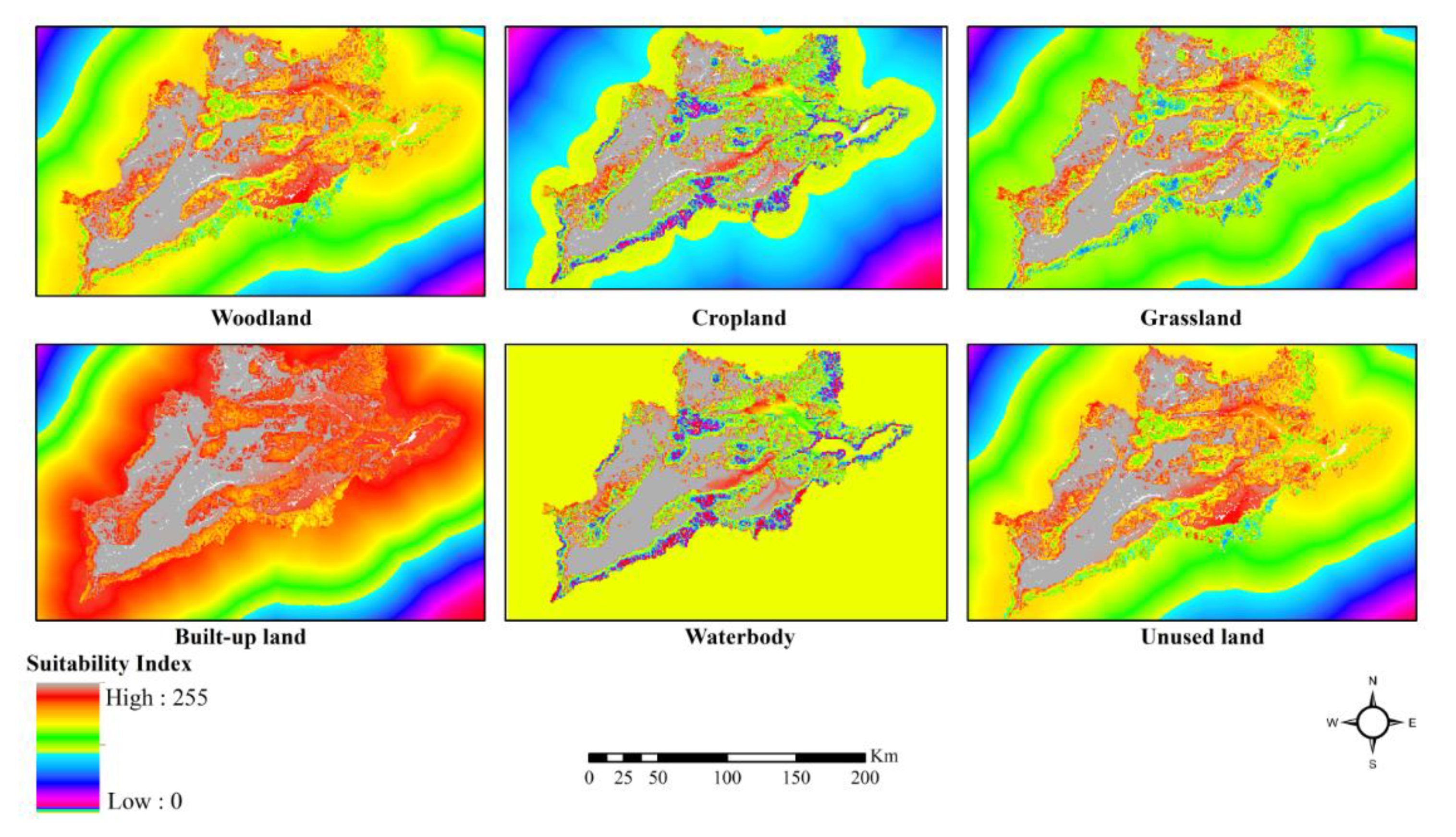
2.2. Simulation of Future LULC Dynamics

LULC prediction involves measuring LULC changes between t₁ and t₂ and extrapolating these changes into the future [36]. The Markov Chain Model is a stochastic progression that analyzes the probability of LULC changes over time by developing a transition probability matrix [24,37,38,39]. Its analysis is a transition probability matrix between t₁ and t₂ that indicates the probability of LULC change from one period to another [40]. The Markov chain process is expressed as [21]

$${\mathrm{F}}_{\mathrm{x}}(\mathrm{X}\left({\mathrm{t}}_{\mathrm{n}+1}\right)\le {\mathrm{x}}_{\mathrm{n}+1}|\mathrm{X}\left({\mathrm{t}}_{\mathrm{n}}\right)={\mathrm{x}}_{\mathrm{n}},\mathrm{X}\left({\mathrm{t}}_{\mathrm{n}-1}\right)={\mathrm{x}}_{\mathrm{n}-1},\dots ,\mathrm{X}\left({\mathrm{t}}_1\right)={\mathrm{x}}_1)=\left(\mathrm{X}\left({\mathrm{t}}_{\mathrm{n}+1}\right)\le {\mathrm{x}}_{\mathrm{n}+1}|\mathrm{X}\left({\mathrm{t}}_{\mathrm{n}}\right)={\mathrm{x}}_{\mathrm{n}}\right)$$

(1)

where X(t) represents the Markov chain process for a particular time (t); t_n defines the present time, while t_n+1 defines the time for changes in the future. Similarly, the notation t_n−1 is used to denote the previous changes.

As described in the previous study [21], Equation (2) denotes the transition probability from state i to state j, while X[k] represents the state k (k = 1,2,3,...)

$${\mathrm{P}}_{\mathrm{i},\mathrm{j}}={\mathrm{P}}_{\mathrm{r}}(\mathrm{X}\left[\mathrm{k}+1\right]=\mathrm{j}|\mathrm{X}\left[\mathrm{k}\right]=\mathrm{i})$$

(2)

If the Markov chain follows a finite number of states (i.e., n), transition probability matrix can be defined as [21]

$$\left[\begin{array}{ccc}{\mathrm{P}}_{1,1}& {\mathrm{P}}_{1,2}& .\\ {\mathrm{P}}_{2,1}& {\mathrm{P}}_{2,2}& .\\ \begin{array}{c}.\\ \begin{array}{c}.\\ {\mathrm{P}}_{\mathrm{n},1}\end{array}\end{array}& \begin{array}{c}.\\ \begin{array}{c}.\\ {\mathrm{P}}_{\mathrm{n},2}\end{array}\end{array}& \begin{array}{c}.\\ \begin{array}{c}.\\ .\end{array}\end{array}\end{array}\begin{array}{ccc}.& .& {\mathrm{P}}_{1,\mathrm{n}}\\ .& .& {\mathrm{P}}_{2,\mathrm{n}}\\ \begin{array}{c}.\\ \begin{array}{c}.\\ .\end{array}\end{array}& \begin{array}{c}.\\ \begin{array}{c}.\\ .\end{array}\end{array}& \begin{array}{c}.\\ \begin{array}{c}.\\ {\mathrm{P}}_{\mathrm{n},\mathrm{n}}\end{array}\end{array}\end{array}\right]$$

(3)

CA–Markov predicts the trend and the spatial structure of different LULC classes [15,41,42,43]. The CA methods are very efficient tools for imitating complex spatial processes based on simple decision rules [44]. Each cell has a particular condition that is influenced by its neighboring cells as well as features of the cell itself [45]. The CA–Markov chain is a combination of the Markov Chain and CA that was developed to solve Markov chain limitation by adding a spatial dimension to the model by CA. In this study, the CA–Markov chain model was used to predict LULC in 2030, 2060, and 2090 in GRB to generate data for understanding future land-use variation in the basin. The IDRISI Selva software v.17 was used for land-use simulation. For developing the CA–Markov model, three types of data, namely, the basic land-cover image, Markov transition areas file, and a collection of transition suitability images, were used. The transition probability matrices were explored with 1980, 1990, 2000, and 2010 LULC maps. Then, the matrices were employed in the prediction of future LULC changes. The LULC transition suitability maps are prepared by combining a collection of maps (factors and constraints) using the multi-criteria evaluation (MCE) method. The Markov module is operated to generate transition areas files before executing a CA–Markov module during the implementation of the Markovian LULC change modeling. The framework of the study is summarized in Figure 2.

A suitability map for each class is considered as a pre-requirement before using the CA. Suitability maps are obtained from the MCE by combining the information from several criteria to form a single index of evaluation [46]. The MCE is a standard strategy for evaluating and collecting weighted maps depending on the specialist’s comprehension of the interactions and impacts of the factors with LULC [46]. The future LULC suitability maps of GRB were prepared, considering the factors responsible for LULC change and distribution. The factors considered were slope, elevation, distance from the road, distance from the motorway, distance from railway [9,21,47,48]. Slope is an important factor because it determines whether the land is useful for humans. For example, agriculture and building require a fairly gentle slope. Elevation is often a good predictor of areas that are suitable for agriculture, and thus lowlands are vulnerable to conversion to agricultural land. Distance from the roads, motorways, or railways facilitates access to remote areas; therefore, building roads promotes anthropogenic disturbances. Water bodies and built-up areas were important parameters in the extraction of suitability maps and were used as constraints. Suitable areas for conversion to each class were assigned by giving the value for the five classes from 0 (no probability for conversion) to 1 (high probability for conversion). The suitability maps for each LULC class are shown in Figure A1.

Factor and constraint maps were processed with ArcGIS Desktop v.10.1; then, the maps were used as inputs of IDRISI Selva v.17 for further processing. During the standardization stage, the values of the factors were converted to a number between 0 and 255, where 0 represents low suitability and 255 denotes high suitability. Appendix A

Table A1. Factors, membership functions, control points, and constraints of the different land use classes. MD: Monotonically Decreasing function.

LULC Class	Factors	Membership Function	Control Points	Constraints
Cropland	Slope	MD-J shape	C = 1.5; d = 3	Water Built-up
	Elevation	Symmetric-Sigmoidal	a = 500; b = 1000 c = 1300; d = 2100
	Distance from road *	MD-Sigmoidal	c = 0; d = max
Grassland	Distance from motorway *	MD-Sigmoidal	c = 0; d = max	Water Built-up
	Distance from road *	MD-Sigmoidal	c = 0; d = max
	Slope	MD-Symmetric	c = 1.5; d = 3
	Elevation	Symmetric-Sigmoidal	a = 500; b = 1000; c = 1300; d = 2100
Water body	Water bodies	No fuzzy
Built up land	Slope	MD-Symmetric	c = 1.5; d = 3	Water
	Elevation	Symmetric-Sigmoidal	a = 500; b = 1000; c = 1300; d = 2100
	Distance from road *	MD-Sigmoidal	c = 0; d = max
	Distance from motorway *	MD-Sigmoidal	c = 0; d = max
	Distance from railways *	MD-Sigmoidal	c = 0; d = max
Unused land	Slope	MD-Symmetric	c = 1.5; d = 3	Water Built-up
	Elevation	Symmetric-Sigmoidal	a = 500; b = 1000; c = 1300; d = 2100
	Distance from road *	MD-Sigmoidal	c = 0; d = max
Woodland	Slope	MD-Symmetric	c = 1.5; d = 3	Water Built-up
	Elevation	Symmetric-Sigmoidal	a = 500; b = 1000; c = 1300; d = 2100
	Distance from road *	MD-Sigmoidal	c = 0; d = max
	Distance from motorway *	MD-Sigmoidal	c = 0; d = max
	Distance from railways *	MD-Sigmoidal	c = 0; d = max

(*) Factors not taken into account in the ‘Governance’ scenario.

presents the details of the factors and constraints considered for each LULC class. The images were classified into two classes, using (a Boolean) 0/1. In the Boolean images, non-constraint and constraint criteria were assigned a value of 1 and 0, respectively. The fussy membership function in IDRISI Selva is used for the standardization of factors and ensuring the logical consistency of the selected factors. The fuzzy membership functions used in this study are sigmoidal, J-shaped, and linear membership functions [46]. For every fuzzy membership function (J-shaped, sigmoid, and linear), the suitability of a given landscape for a specific LULC bears specific shapes as the value of a factor increases. These are as follows: [4] as the value of the factor increases, the suitability of a land surface for a given LULC category increases (monotonically increasing); (2) as the value of the factor increases, the suitability of a land surface for a given LULC category decreases (monotonically decreasing). The weighted overlay of factors can be carried out using three approaches: user-defined weights, equal weights, and analytic hierarchy process (AHP) [49,50]. The AHP is a multi-criteria and multi-objective decision-making technique, which facilitates the aggregation of constraints and factors using the weighted linear combination (WLC) algorithm [51]. The AHP approach has been widely used in LULC change prediction [21,40,43,49,52,53]. In this study, we adopted the AHP approach. The WLC aggregation under the MCE generated the standardized suitability maps for every LULC class. The suitability maps for each LULC class are shown in Figure A1.

2.3. Scenarios Setting and Model Validation

The land system change under different levels of socioeconomic development was captured by developing two scenarios according to the historical trend of land system change from 1980 to 2010. At one end, the first scenario, BAU, which assumed that recent socioeconomic development trends (rapid urbanization and increase of population) would continue. Distance from the road, distance from the motorway, distance from the railway, slope, and elevation were the driving factors of this scenario. At the other end, a more idealized and controlled picture is the Gov scenario that assumed an environment-friendly, controlled LULC change planning is implemented in the whole basin. In this scenario, drivers such as distance from the road, distance from the motorway, and distance from the railway are assumed to be negligible in the model due to the implemented strict regulations on infrastructure development induced disturbances. We supposed that the growth and expansion of urban centers are limited in this scenario. Therefore, the remaining influencing factors to LULC change are slope and elevation. These scenarios are just projections of different development pathways, which can be supported and validated with socio-economic and census data for a critical understanding of the possible LULC change processes in GRB. The scenarios are implemented in Idrisi Selva v.17 by taking into account the factors and constraints driving each scenario (Appendix A Table A1). Consequently, we used the LULC maps in 2000 and 2010 as input in the CA–Markov model. Future annual LULC distribution of each scenario is then simulated for 2030, 2060, and 2090.

When predicting future decadal changes where no datasets are available for assessing the accuracy of the simulation, model calibration and validation are a fundamental component in the modeling process [40,43,47,54]. There are several methods used for validating future LULC change prediction models. Such methods include the kappa coefficient (κ) and Cramér’s V [23,55], quantity disagreement and allocation disagreement approach [23,55,56], and Chi-Square–F-test of two images for variance [57,58]. In this study, the kappa coefficient was implemented, and the model was validated after simulating the 2010 LULC conditions using the 1990 and 2000 LULC maps. The accuracy of the simulated 2010 LULC map was assessed using the VALIDATE and CROSSTAB module in IDRISI to estimate the level of agreement between the simulated map and the reference map of 2010. CROSSTAB uses a cell-by-cell method, expressed by the Kappa Index of Agreement [59,60]. Hence, Kappa indexes such as Kappa for no information (Kno), Kappa for location (Klocation), and Kappa for standard (Kstandard) [61,62,63] were used to compare the agreements of the two maps with the VALIDATE module. The use of Kappa indexes for the assessment determines the overall success rate, and it provides an understanding of the practical factors in the strength or weakness of the results. When 0.75 ≤ Kappa < 1, the maps are in a high level of agreement; if 0.5 ≤ Kappa ≤ 0.75, it has a medium level of agreement; and if Kappa ≤ 0.5, it has a rare agreement [54,62]. After obtaining successful Kappa values, the CA–Markov model was adopted and then used to simulate the LULC maps of 2030, 2060, and 2090 under BAU and Gov scenarios.

The equations below express the summary statistics for the Kappa variations according to Omar et al. [64]

$$Kno=\left(M\left(m\right)N\left(n\right)\right)/P\left(p\right)-N\left(n\right)),$$

(4)

$$Klocation=\left(M\left(m\right)N\left(n\right)\right)/P\left(p\right)-N\left(n\right)),$$

(5)

$$\mathrm{and}Kstandard=\left(M\left(m\right)N\left(n\right)\right)/P\left(p\right)-N\left(n\right))$$

(6)

where no information is defined by N(n), medium grid cell-level information by M(m), and perfect grid cell-level information across the landscape by P(p).

LULC is usually carried out to show the patterns of change, which is essential for decision-makers. A comparison of land-use in different periods and under different scenarios was made after successful simulation of LULC in 2030, 2060, and 2090. A cross-tabulation procedure between the classifications was processed with IDRISI Selva V.17 [63]. Conversion matrix [40,65], between 1980 and 1990, between 1990 and 2000, and between 2000 and 2010, were also performed in order to analyze the decadal variation in each land-use/land-cover category. Furthermore, percent change [47] was also computed to show the magnitude of the changes happening between different periods, and this was achieved using Equations (7) and (8), respectively,

$$Change (\%)=\left(\frac{X_2-X_1}{1}\right)\times 100$$

(7)

$$\mathrm{and}RC=\left(\frac{X_2-X_1}{Y}\right),$$

(8)

where RC is the rate of change from time 1 to time 2 (km²/year), X₂ is the area of LULC (km²) in time 2, X₁ is the area of LULC (km²) in time 1, and Y is the time interval between X₁ and X₂ in years.

3. Results and Discussion

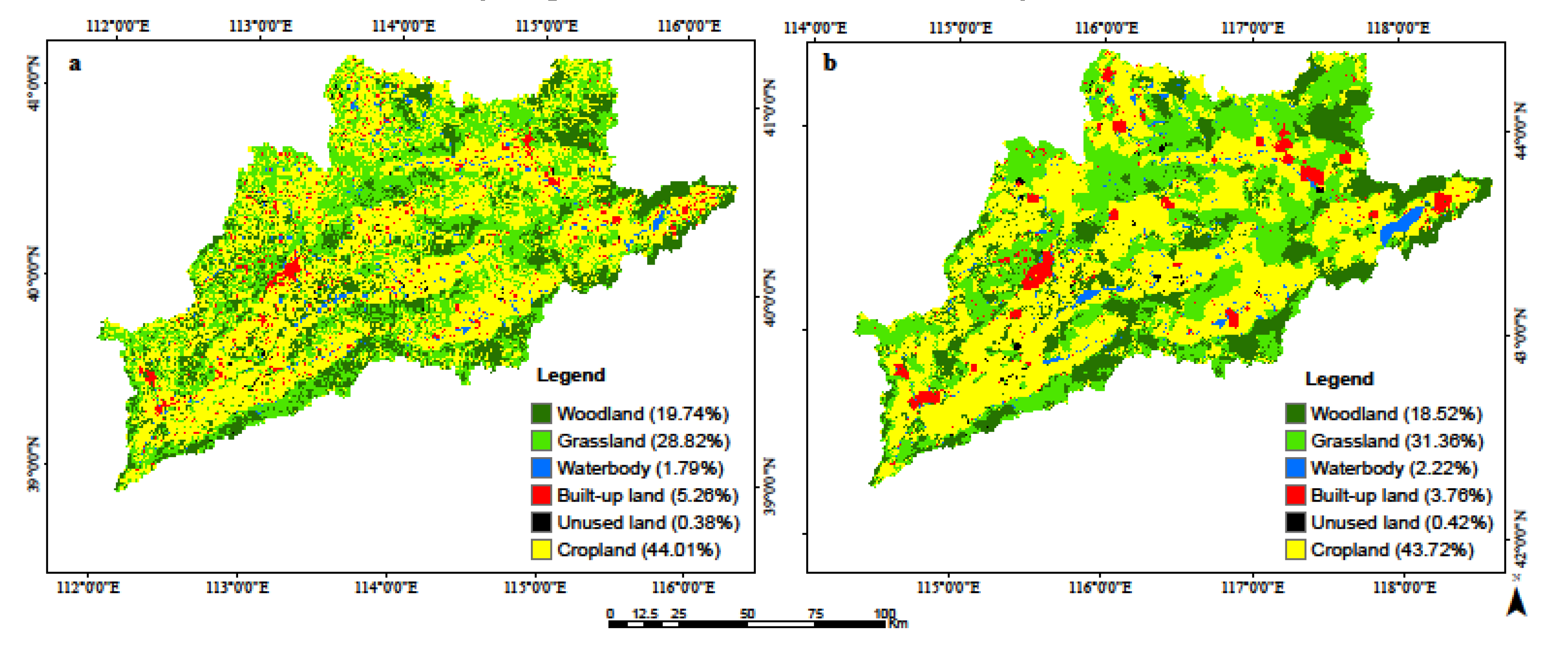
3.1. CA-Markov Model Validation

Figure 3a,b shows a comparison of the simulated and actual maps in 2010. The result shows a close similarity between the two maps in terms of the spatial distribution of LULC. In particular, the modeled agricultural and water body areas agree very well with the observations (Figure 3). Figure 4 shows the total area of simulated and actual LULC classes in 2010. The area extent of the simulated and actual maps also attests to the likeness between the two maps. The proportions of woodland, cropland, water body, and unused land of the simulated map are similar to those of the actual map. For instance, woodland is modeled to account for 18.52% of the total area, which is close to the actual percentage, 19.74% (Figure 4). However, some LULC classes were less accurately simulated. For example, grassland was over-projected, while built-up was slightly underestimated (Figure 4). A possible explanation of the poor simulation of built-up areas might be the inability of the model to capture the newly developed areas without assimilating the detailed information on urbanization. However, from these results, it can be deduced that the model can simulate past LULC well. To quantitatively estimate the level of agreement between the simulated and actual map of 2010, we used three Kappa indices, namely, Kno, Kstandard, and Klocality. The analysis assessed with VALIDATE module showed a good performance with Kno = 0.9110, Klocation = 0.8887, and Kstandard = 0.8794.

Table 2. Comparison of KIA indices for simulated and actual LULC categories.

LULC Category	KIA 1	LULC Category	KIA
Woodland	0.8530	Built-up land	0.6013
Grassland	0.7999	Unused land	0.8485
Water body	0.9245	Cropland	0.7916
Overall KIA	0.8794

¹ KIA: Kappa Index of Agreement.

displays a cell-by-cell comparison of land use classes between the simulated map and the actual map. KIA showed a good result for all LULC categories, ranging from 0.60 to 0.92 for the built-up and water body classes, respectively. In general, the indices performed well quantitatively and spatially, which can be described as almost perfect agreement. The results provide clear evidence that CA–Markov can predict future LULC in GRB. Good agreement of all Kappa indexes for the assessment not only projects the overall ability of the model to simulate a past LULC, but also shows its ability to predict future LULC effectively.

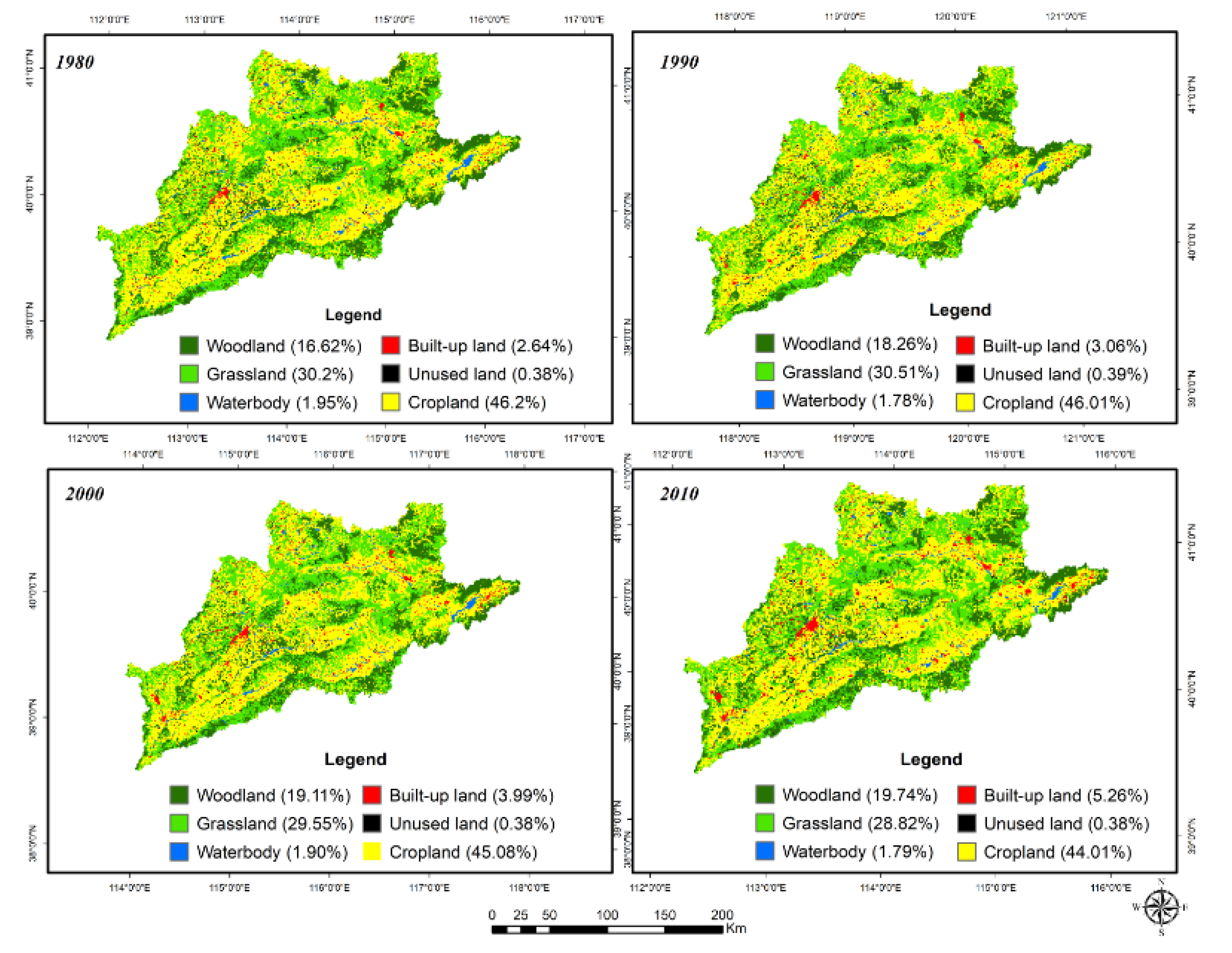
3.2. Land Use/Land Cover Change from 1980–2010

Table 3. Distributions of land use/land cover classes in Guanting Reservoir from 1980 to 2010.

LULC	1980		1990		2000		2010
	Area (Km2)	Area (%)	Area (Km2)	Area (%)	Area (Km2)	Area (%)	Area (Km2)	Area (%)
Woodland	8129	18.62	7970	18.26	8345	19.11	8616.92	19.74
Grassland	13,186.3	30.20	13,318	30.51	12,899.3	29.55	12,582.98	28.82
Water body	853	1.95	776	1.78	829	1.90	780.49	1.79
Built-up	1154	2.64	1335	3.06	1740	3.99	2296.99	5.26
Unused land	164	0.38	171	0.39	165	0.38	167.34	0.38
Cropland	20,171	46.20	20,087	46.01	19,679	45.08	19,212.61	44.01

shows the area and percentage of land-use change from 1980 to 2010. Cropland, grassland, and woodland were the predominant land-use classes in the study area, covering more than 90% of the total area. Built-up land, water body, and unused land accounted only for a small portion. For instance, in 1980, cropland covered 20,171 km², representing 46.2% of the study region, while grassland and woodland span 13,186.3 km² (30.2%) and 8129 km² (18.62%), respectively. During the same period, the smallest portions, namely built-up, water body, and unused land, covered only 2.64%, 1.95%, and 0.38% of the region, respectively. The next decades showed a different trend, with slight changes in some proportions. Built-up land and woodland coverage expanded, while grassland and cropland areas declined. Specifically, from 1990 to 2010, built-up land nearly doubled its proportion, rising from 3.06% to 5.26%. This increase might be adequately explained by population growth, which contributes to the construction of new infrastructures such as houses, hospitals, and schools. One contributing factor to this rise could be the rapid urbanization, which leads to cultivated land loss in the region [66,67,68,69]. In fact, in the 1990s, the Chinese government improved infrastructure and road transportation in the whole basin; therefore, urbanization expanded further into the peripheral areas at the expense of grassland and cropland [70]. Shi et al. [17] reached a similar conclusion by pointing out that the urbanization rate increased in the Haihe River basin from 29% to 36% during that period and will continue to grow more in the future. The percentage covered by each LULC from 1980 to 2010 is shown in

Table 4. Percent changes in LULC classes that occur in the Guanting Reservoir Basin.

LULC	1980–1990	1990–2000	2000–2010	1980–2010
Woodland	−1.96	−0.31	+3.26	+6.00
Grassland	+1.00	−0.14	−2.45	−4.58
Water body	−9.03	6.83	−5.85	−8.50
Built-up	+15.68	+0.37	+32.01	+99.05
Unused land	+4.27	−3.51	+1.42	+2.04
Cropland	−0.42	−0.04	−2.37	−4.75

. Woodland increased at a rate of 6% from 1980 to 2010. This increase was probably the effect of the “Grain for Green” policies taken by the Government [35,71], along with the “Project on Sand Prevention and Desertification Control” around Beijing [72]. This result is in accord with the study by Shi et al. [17], who noted that woodland increased by 2.7% in the same region around the 1990s and 2000s. Contrarily, as displayed in Table 4, grassland decreased from 30.2% in 1980 to 28.82% in 2010, while shrinkage of 8.5% is noticed in water body coverage over the same period (1980–2010). It is worth noting that water body areas are mainly rivers, reservoirs, lakes, and ponds, which are primarily used for irrigation. These findings are consistent with the other studies [10,14,16,31,69,73,74] in Northern China, confirming the depletion of dense grasslands and water bodies. Throughout the years, unused land occupying the mountainous areas, which are mainly composed of sandy lands, did not change much compared to other LULC classes.

3.3. LULC Transition Probabilities Matrices

LULC conversion from one category to another is frequent in LULC studies [34,35]. The changes are displayed in an n-by-n LULC class matrix, in which rows show the previous land cover classes at the time 1, while the columns represent the latter land cover classes at time 2. The off-diagonal values indicate the probability of a change occurring from one land use cover to another from time 1 to time 2. However, the diagonals represent the probability of a given LULC class to remain stable after a given time from time 1 to time 2. The changes of one LULC category to another between 1980–1990, 1990–2000, and 2000–2010 periods are shown in the tables below.

3.3.1. Conversion between 1980 and 1990

Table 5. Transition probabilities of LULC classes from 1980 to 1990.

1980	1990
	Wood	Grass	Water	Built	Unused	Crop
Wood 1	0.4972	0.2782	0.0073	0.2059	0.0015	0.0098
Grass 2	0.154	0.5	0.0096	0.0167	0.3154	0.0043
Water 3	0.0845	0.5067	0.2411	0.0012	0.1354	0.031
Built 4	0.0378	0.6346	0.0198	0.1694	0.0054	0.133
Unused 5	0.0635	0.4194	0.0064	0.0191	0.305	0.1866
Crop 6	0.0949	0.2269	0.0239	0.0554	0.0047	0.5941

¹ Wood: woodland; ² Grass: Grassland; ³ Water: Water body; ⁴ Built: built-up land; ⁵ Unused: Unused land; ⁶ Crop: Cropland.

displays the transition probabilities of LULC classes from 1980 to 1990. The diagonal line showed the probabilities of LULC classes to remain unchanged in 1990. The LULC classes with high probabilities to remain stable are grassland, cropland, and woodland, accounting for 50%, 59%, and 49% of their original areas, respectively. Built-up land has the lowest probability of remaining unchanged, with a considerable portion converted to grassland (63.4%) from 1980 to 1990, although other LULC classes were converted to built-up too. The probability matrix in Table 5 showed that none of the LULC categories were reverted to water body class; however, water body was moderately converted to grassland (50.67%), highlighting the fact that waterbody has been substantially occupied by agriculture, industries, and households in this region during this period. In Table 5, some portions of grassland were transformed into unused land, which slightly increased its percentage; this shows how green areas were slowly depleted. Overall, slight changes in LULC occurred from 1980 to 1990, and the LULC classes with increasing coverage were grassland, built-up land, and unused land.

3.3.2. Conversion between 1990 and 2000

Table 6. Transition probabilities of LULC classes from 1990 to 2000.

1990	2000
	Wood	Grass	Water	Built	Unused	Crop
Wood 1	0.5024	0.2603	0.2174	0.0075	0.0014	0.011
Grass 2	0.159	0.5018	0.0098	0.3094	0.0045	0.0156
Water 3	0.0702	0.139	0.2651	0.4927	0.0014	0.0317
Built 4	0.0499	0.1264	0.0211	0.6149	0.0023	0.1853
Unused 5	0.0609	0.2923	0.0061	0.4202	0.1839	0.0365
Crop 6	0.0917	0.2301	0.0255	0.0537	0.0044	0.5945

¹ Wood: woodland; ² Grass: Grassland; ³ Water: Water body; ⁴ Built: built-up land; ⁵ Unused: Unused land; ⁶ Crop: Cropland.

illustrates the LULC transition probability matrix from 1990 to 2000. The information generated from this table indicates that 42% of the unused land was converted into built-up land from 1990 to 2000. Similarly, 31% and 49.2% of grassland and water body areas were also converted to built-up land. The increase in built-up land may be attributed to the urbanization growth and population rise in the region, as pointed out in the other studies [27,68,69]. Additionally, Liu, Liu, Zhuang, Zhang and Deng [35], and Tan, Li, Xie and Lu [26] confirmed that the population growth and associated decline in cropland were the most critical factors for the change in LULC. These findings are also confirmed by Liu, Liu, Tian, Zhuang, Zhang, Zhang, Tang and Deng [34] and Tan, Li, Xie and Lu [26] who reported that in the 1990s, the region faced significant exploitation of natural resources such as water, land, forests, leading to LULC change. All these changes might also influence hydrological components in the reservoir. As an example, Yang and Tian [74] indicated that the variation in agricultural land and agricultural water use is the most probable driving factors of runoff decline in the reservoir. Wang et al. [75] went further, demonstrating that land-use change was responsible for a 7.9% decrease in surface water volumes in the basin during the period 1991–2000. Unused land indicated the highest transformation percentage, with a probability of only 18.3% to remain unchanged, meaning that it may be converted to other classes. Woodland remained relatively stable, with a probability of 50.24%. Similarly, grassland and cropland displayed 50.18% and 59.45% probability of remaining as respective grassland and cropland classes.

3.3.3. Conversion between 2000 and 2010

Table 7. Transition probabilities of LULC classes from 2000 to 2010.

2000	2010
	Wood	Grass	Water	Built	Unused	Crop
Wood 1	0.444	0.0223	0.0001	0.1224	0.2001	0.2111
Grass 2	0.0447	0.3658	0.0087	0.5384	0.007	0.0354
Water 3	0.0107	0.0293	0.3448	0.0201	0.0001	0.595
Built 4	0.0977	0.0167	0.0158	0.4374	0.0159	0.4165
Unused 5	0.0002	0.1886	0.0305	0.3003	0.4794	0.0009
Crop 6	0.08	0.0388	0.0023	0.6098	0.0035	0.2656

¹ Wood: woodland; ² Grass: Grassland; ³ Water: Water body; ⁴ Built: built-up land; ⁵ Unused: Unused land; ⁶ Crop: Cropland.

shows the transition probability of LULC between 2000 and 2010. It was observed that 60.9% and 53.8% of cropland and woodland were converted to built-up area, respectively. Woodland experienced significant conversion, where 21.1% were transformed to cropland, 20% to unused land, and 12.2% to cropland. One possible explanation might be the deforestation in the region caused by urbanization (housing and other infrastructure). Similar conclusions were reached earlier by Li, Deng, Yin and Yang [16] and Shi, Xiao, Shen and Yamaguchi [17], who found that the land-use change is principally dominated by the conversion of cultivated land and forest to built-up area in northern China. Once again, rapid population growth, improvement in transport infrastructure, and expansion of peripheral cities accelerated the process of urbanization in the region, resulting in a significant change in built-up land. During the same period, 41.6% of built-up land and 59.5% of water body area were both transformed into cropland. This conversion is because irrigation takes a considerable part of water consumption in GRB; therefore, it is obvious to notice a conversion of water body into agricultural land. In summary, GRB experienced a transformation of LULC from grassland, cropland, and woodland to built-up, and from water body to cropland, making up the 2010 LULC.

Eastman [46] opposed the idea that one of the fundamental spatial elements that underlie the dynamics of many change events is proximity; therefore, areas will have a higher tendency to change to a class when they are near existing areas of the same category [21,39]. It is often the case that some LULC data exhibit spatial autocorrelation, though the LULC classes are independent to each other [76]. A cellular entity will independently vary its state based on its previous state and that of its immediate local neighbors [46]. In GRB, cropland and grassland are neighbored by unused land and built-up areas. Agricultural practices are carried out along water bodies (pounds, lakes, wetland). During dry seasons, these areas are easily used for agriculture; therefore, based on neighborhood relationships, it is ordinary to observe conversion from water body to cropland or vice versa, as shown in Table 7.

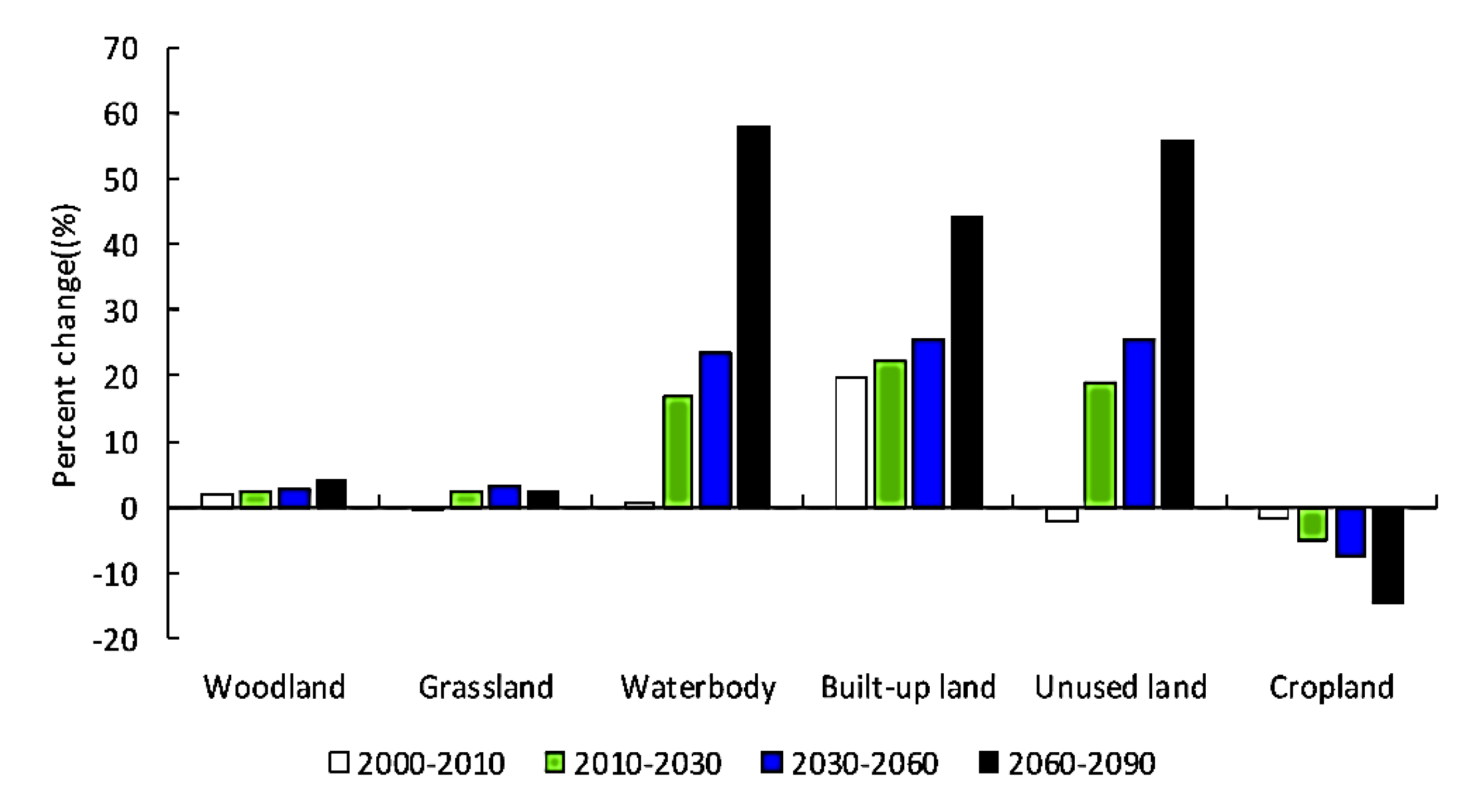
3.4. Future LULC Dynamics

Two scenarios were developed according to historical patterns of LULC change from 1980 to 2010 to capture the LULC change under different levels of socioeconomic development. Therefore, the LULC changes of 2030, 2060, and 2090 under the BAU and Gov scenarios were developed in GRB and presented in Figure 5. In the BAU scenario, we assumed that recent socioeconomic development trends would continue, whereas the Gov scenario assumes that a more regulated development is implemented in GRB. In the Gov scenario, drivers such as distance from the road, distance from the motorway, and distance from railway are not taken into account in the model in order to minimize the influence of infrastructure-development-induced further LULC changes. The only influencing factors to LULC change in the Gov scenario are slope and elevation. Figure 5 displays the LULC of GRB in 2030, 2060, and 2090 under the BAU and Gov scenarios. Contrary to the Gov scenario, the BAU scenario projected a significant increase in urban cities, decades after decades in the plain region, rising from 2296.98 km² (5.26%) in 2010 to 11,757.35km² (26.93%) in 2090 (Figure 6). The projections of future urbanization will increase if new roads, highways, and industries are constructed on the current farming regions. Cropland will be destroyed and transformed into small cities and industries if the current rate of urbanization and industrialization continues. This trend shows that there is a need for efficient and environmental-friendly urbanization planning in both urban and rural areas. Moreover, from 2010 to 2090, both cropland and grassland are projected to decrease sharply to 42% and 28%, respectively, under the BAU scenario. This situation may be attributed to the expansion of urban areas, as mentioned earlier. In this scenario, it is essential to take necessary actions for land protection and taking into consideration the needs of farmers who will suffer the most by these changes. With the growing population expected in the future decades, the region will face a high demand for food. To tackle these challenges, efficient systems of agricultural practices such as crop rotation and polycultures, agroforestry (growing shrubs amongst plants and vegetables to increase crop yields), and sustainable farming (using renewable energy for pumping and irrigation systems) could be implemented. Additionally, a sustainable land management system with the participation of local farmers and all stakeholders will be beneficial. Coordination between provinces would be important to implement national policies regarding food and water security efficiently. Despite the increase in the built-up area, a slight increase in the woodland area is projected, especially in 2030 (8786.27km²) and in 2090 (up to 10,030km²) (Figure 6), which accounts for an increase of 2.85% (

Table 8. Projected percent changes in LULC classes in GRB from 2000 to 2090 under the BAU and Gov scenarios.

LULC Category	Reference	BAU			Gov
	2010	2030	2060	2090	2030	2060	2090
Woodland	19.74	20.13	22.51	22.98	19.03	19.59	20.34
Grassland	28.82	28.78	24.65	20.63	31.15	32.12	32.86
Water body	1.79	1.77	1.92	2.11	2.09	2.58	4.07
Built-up land	5.26	7.91	17.98	26.93	4.47	5.61	8.08
Unused land	0.38	0.60	1.24	1.96	0.46	0.57	0.89
Cropland	44.01	40.81	31.70	25.39	42.81	39.53	33.76

). Therefore, some of the green areas would still exist.

Under the Gov scenario, necessary water planning and management policies are taken, and an increase in water body coverage is observed across the whole basin by 2.09% to 4.07% from 2010 to 2090 (Table 8). Irrigated agricultural land could have created more areas covered by water. Under this scenario, water resources allocated for agricultural practices and industrial uses are well planned by taking into consideration the protection of the environment. Assuming that reservoirs are built across the basin to store enough water during the rainy season, the South-North Water Diversion Project is efficiently working, and pumping underground water is well regulated; this could lead to efficient water management in the basin, as displayed in 2090. From 2030 to 2090, conservation measures projected in the Gov scenario would also increase unused land (0.47% to 0.89%), which could be later transformed into recreational, green, or protected areas. If current trends continue, increase in unused land will probably continue into the next century. Figure 7 displays the percent change in LULC under the Gov scenario. We note that cropland decreases decades after decades, up to 15% of decrease between 2060 and 2090. At the same time, water body, unused land, and built-up land show the highest increase in the LULC area. They all have an incremental trend from 2000 to 2090. Woodland follows the same pattern despite its minor increase throughout the decade, but grassland slightly decreases from 2060 to 2090. Agricultural land drops while urban areas and water body increase. The expansion of the built-up area under this scenario has nothing to do with the one observed in the BAU scenario, which was more prominent. A transition probability matrix would have been a necessity to indicate the conversion between different LULCs in both scenarios. We would carry further studies toward that aim. Under all scenarios, future urbanization is concentrated in western and northern regions, where the density of cities will continue for several decades along the Sang River and Yang River. The well-being of the region highly depends on the successful protection of vulnerable areas (woodland and water body) and the programs put in place to protect them.

3.5. Uncertainty Analysis

Using the Kappa indices to evaluate the projected maps, causes are not unanimously accepted in the field of LULC change modeling because of the randomness of its comparison. Summarizing the cross-tabulation matrix in terms of quantity of disagreement and allocation disagreement is, therefore, the best option [55]. Another uncertainty is related to the variation in accuracy within clusters. Usually, the model predicts the change in the wrong location, which improves the percentage of the correctness of models used in a small quantity of change compared to models applied in a large quantity of change [77]. The maps obtained under the LULC scenarios in this study are only projections of different socio-economic pathways for the basin. They are intended to support decision-making regarding LULC policies and water management. Predicting LULC is vital in providing necessary information to obtain a deeper understanding of the land-use system, as well as for effective land use planning and water resources management. The limitation of this study was mostly related to the model used to predict LULC change. The CA–Markov model projects future LULC distributions based on current trends, while future patterns are uncertain due to factors such as population growth, a shift in socio-economic development, and natural hazards. The projections of development pathways used in this study lack socio-economic and census data for a complete analysis of and understanding of LULC change processes. The spatial planning map of GRB would have been useful, as it portrays a realistic LULC planification of the study area. Future work could focus on assessing uncertainties related to the projections using a logistic regression model or geographically weighted regression. However, we are confident that the research methodology used in this study is reliable. The results should be interpreted as a hypothetical fate of future LULC change in GRB if the same conditions are followed. Although the reliability of land use projections starts to reduce with time when the period of simulation exceeds ten years [78], the long-term projections of LULC simulated in this study are useful because they provide an overview of the future LULC changes in GRB. However, the use of two opposite LULC scenarios (BAU and Gov) reduces and quantifies the uncertainties associated with the model, thus enhancing the applicability of simulation results. This method is better than just relying on a single scenario.

4. Conclusions

In this study, the CA-MARKOV model has been used to predict two scenarios—BAU and Gov—of the future LULC system in Guanting River Basin using historical maps from 1980 to 2010. To the best of our knowledge, this study is the first one for the GRB. Therefore, the model developed in this study is essential as it can be useful for LULC planners and water resources managers to identify the fragile ecological systems and take proper measures. Firstly, the accuracy of the model is tested by comparing the actual 2010 LULC map with its simulated counterpart using the 1990 and 2000 LULC maps. Overall, the validation shows a satisfactory result, which indicates that the CA–Markov model can be used to simulate future LULC in GRB. A significant amount of LULC conversions had occurred from 1980 to 2010 in GRB. Built-up and woodland areas have increased from 1980 through 2010. An increase in built-up land was probably due to the rapid population growth, improvement in transport infrastructure, and expansion of peripheral cities. In contrast, grassland, water body, and cropland have declined in coverage, while unused land did not change much during the same period. When facing such land-cover changes, projecting future changes under various assumptions is critical for efficient decision-making. Such scenarios also contribute to increasing awareness of the ecological consequences of growing pressures; therefore, we developed two LULC scenarios (BAU and Gov) in this study. Under the BAU scenario, which assumed that the current socioeconomic development trends would continue, urbanization is projected to increase significantly in 2030, 2060, and 2090. In contrast, cropland and grassland are projected to decrease sharply. If this scenario persists, it will have a severe impact on the environment, soils, and water resources in the whole basin. Under the Gov scenario, LULC changes are more moderate and slower, and water body area and unused land will increase significantly from 2030 to 2090. This scenario assumes that water resources allocated for agricultural practices and industrial uses are well planned. Therefore, we recommend following the Gov scenario, which is environmentally sustainable and economically profitable for the GRB in the long term.

References

1. McCuen, R.H. Modeling Hydrologic Change: Statistical Methods; CRC Press: Boca Raton, FL, USA, 2016. [Google Scholar]
2. Behera, M.D.; Borate, S.N.; Panda, S.N.; Behera, P.R.; Roy, P.S. Modelling and analyzing the watershed dynamics using cellular automata (ca)–markov model–a geo-information based approach. J. Earth Syst. Sci. 2012, 121, 1011–1024. [Google Scholar] [CrossRef] [Green Version]
3. Zhang, L.; Walker, G.R.; Dawes, W.R. Water balance modelling: Concepts and applications. ACIAR Monogr. Ser. 2002, 84, 31–47. [Google Scholar]
4. Zhang, Y.-K.; Schilling, K. Increasing streamflow and baseflow in mississippi river since the 1940 s: Effect of land use change. J. Hydrol. 2006, 324, 412–422. [Google Scholar] [CrossRef]
5. Zhang, K.; Castanho, A.; Galbraith, D.R.; Moghim, S.; Levine, N.; Bras, R.L.; Coe, M.; Costa, M.H.; Malhi, Y.; Longo, M.; et al. The fate of amazonian ecosystems over the coming century arising from changes in climate, atmospheric co2 and land-use. Glob. Chang. Biol. 2015, 21, 2569–2587. [Google Scholar] [CrossRef] [PubMed]
6. Mohmmed, N.; Zhang, K.; Kabenge, M.; Keesstra, S.; Cerda, A.; Reuben, M.; Elbashier, M.M.A.; Dalson, T.; Ali, A.A.S. Analysis of drought and vulnerability in the north darfur region of sudan. Land. Degrad. Dev. 2018, 29, 4424–4438. [Google Scholar] [CrossRef]
7. Giri, C.; Defourny, P.; Shrestha, S. Land cover characterization and mapping of continental southeast asia using multi-resolution satellite sensor data. Int. J. Remote Sens. 2003, 24, 4181–4196. [Google Scholar] [CrossRef]
8. Verburg, P.H.; de Nijs, T.C.; van Eck, J.R.; Visser, H.; de Jong, K. A method to analyse neighbourhood characteristics of land use patterns. Comput. Environ. Urban Syst. 2004, 28, 667–690. [Google Scholar] [CrossRef]
9. Hyandye, C.; Mandara, C.G.; Safari, J. Gis and logit regression model applications in land use/land cover change and distribution in usangu catchment. Am. J. Remote Sens. 2015, 3, 6–16. [Google Scholar] [CrossRef] [Green Version]
10. Chen, Y.; Li, X.; Su, W.; Li, Y. Simulating the optimal land-use pattern in the farming-pastoral transitional zone of northern China. Comput. Environ. Urban Syst. 2008, 32, 407–414. [Google Scholar] [CrossRef]
11. Xu, X.; Gao, Q.; Liu, Y.-H.; Wang, J.-A.; Zhang, Y. Coupling a land use model and an ecosystem model for a crop-pasture zone. Ecol. Model. 2009, 220, 2503–2511. [Google Scholar] [CrossRef]
12. Huang, Q.; He, C.; Liu, Z.; Shi, P. Modeling the impacts of drying trend scenarios on land systems in northern china using an integrated sd and ca model. Sci. China Earth Sci. 2014, 57, 839–854. [Google Scholar] [CrossRef]
13. Deng, X.; Huang, J.; Lin, Y.; Shi, Q. Interactions between climate, socioeconomics, and land dynamics in qinghai province, China: A lucd model-based numerical experiment. Adv. Meteorol. 2013, 2013, 1–9. [Google Scholar] [CrossRef] [Green Version]
14. Liu, Z.; Verburg, P.H.; Wu, J.; He, C. Understanding land system change through scenario-based simulations: A case study from the drylands in northern china. Environ. Manag. 2017, 59, 440–454. [Google Scholar] [CrossRef] [PubMed]
15. Li, S.H.; Jin, B.X.; Wei, X.Y.; Jiang, Y.Y.; Wang, J.L. Using ca-markov model to model the spatiotemporal change of land use/cover in fuxian lake for decision support. ISPRS Ann. Photogramm. Remote Sens. Spat. Inf. Sci. 2015, 163–168. [Google Scholar] [CrossRef] [Green Version]
16. Li, Z.; Deng, X.; Yin, F.; Yang, C. Analysis of climate and land use changes impacts on land degradation in the north china plain. Adv. Meteorol. 2015, 2015, 1–11. [Google Scholar] [CrossRef]
17. Shi, Y.; Xiao, J.; Shen, Y.; Yamaguchi, Y. Quantifying the spatial differences of landscape change in the hai river basin, China, in the 1990s. Int. J. Remote Sens. 2012, 33, 4482–4501. [Google Scholar] [CrossRef]
18. Wang, R.; Hou, H.; Murayama, Y. Scenario-based simulation of tianjin city using a cellular automata–markov model. Sustainability 2018, 10, 2633. [Google Scholar] [CrossRef] [Green Version]
19. Wu, Q.; Li, H.-Q.; Wang, R.-S.; Paulussen, J.; He, Y.; Wang, M.; Wang, B.-H.; Wang, Z. Monitoring and predicting land use change in beijing using remote sensing and gis. Landsc. Urban Plan. 2006, 78, 322–333. [Google Scholar] [CrossRef]
20. Eastman, J.R. Idrisi Kilimanjaro: Guide to Gis and Image Processing; Clark Labs-Clark University: Worcester, MA, USA, 2003. [Google Scholar]
21. Memarian, H.; Balasundram, S.K.; Bin Talib, J.; Sung, C.T.B.; Sood, A.M.; Abbaspour, K. Validation of ca-markov for simulation of land use and cover change in the langat basin, malaysia. J. Geogr. Inf. Syst. 2012, 4, 542–554. [Google Scholar] [CrossRef] [Green Version]
22. Mas, J.-F.; Paegelow, M.; De Jong, B.; Masera, O.; Guerrero, G.; Follador, M.; Olguin, M.; Diaz, J.; Castillo, M.; Garcia, T. Modelling Tropical Deforestation: A Comparison of Approaches. In Proceedings of the 32rd Symposium on Remote Sensing of Environment, San José, Costa Rica, Jun 2007. [Google Scholar]
23. Baysal, G. Urban Land Use and Land Cover Change Analysis and Modeling a Case Study Area Malatya, Turkey; University of Jaume: Castelon, Spain, 2013. [Google Scholar]
24. López, E.; Bocco, G.; Mendoza, M.; Duhau, E. Predicting land-cover and land-use change in the urban fringe: A case in morelia city, mexico. Landsc. Urban Plan. 2001, 55, 271–285. [Google Scholar]
25. Houet, T.; Hubert-Moy, L. Modeling and Projecting Land-Use and Land-Cover Changes with Cellular Automaton in Considering Landscape Trajectories. Eur. Assoc. Remote Sens. Lab. 2006, 5, 63–79. [Google Scholar]
26. Tan, M.; Li, X.; Xie, H.; Lu, C. Urban land expansion and arable land loss in china—A case study of beijing–tianjin–hebei region. Land Use Policy 2005, 22, 187–196. [Google Scholar] [CrossRef]
27. Jiang, Q.; Deng, X.; Zhan, J.; He, S. Estimation of land production and its response to cultivated land conversion in north china plain. Chin. Geogr. Sci. 2011, 21, 685–694. [Google Scholar] [CrossRef]
28. Zhu, H.-Y.; He, S.-J.; Zhang, M. Driving forces analysis of land use change in bohai rim. Geogr. Res. 2001, 20, 669–678. [Google Scholar]
29. Xiao, J.; Shen, Y.; Ge, J.; Tateishi, R.; Tang, C.; Liang, Y.; Huang, Z. Evaluating urban expansion and land use change in shijiazhuang, China, by using gis and remote sensing. Landsc. Urban Plan. 2006, 75, 69–80. [Google Scholar] [CrossRef]
30. He, W.; Chen, S.; Liu, X.; Chen, J. Water quality monitoring in a slightly-polluted inland water body through remote sensing—case study of the guanting reservoir in Beijing, China. Front. Environ. Sci. Eng. China 2008, 2, 163–171. [Google Scholar] [CrossRef]
31. Zhang, K.; Ruben, G.B.; Li, X.; Li, Z.; Yu, Z.; Xia, J.; Dong, Z. A comprehensive assessment framework for quantifying climatic and anthropogenic contributions to streamflow changes: A case study in a typical semi-arid north china basin. Environ. Model. Softw. 2020, 128, 104704. [Google Scholar] [CrossRef]
32. Otto, I.M.; Wechsung, F.; Wang, X.; Möhring, J.; Tan, R. Water scarcity impacts and challenges of water governance in the guanting basin, north china. Evidence from interviews with local stakeholders. In Integrated Water Resources Management: Concept, Research and Implementation; Springer: Berlin/Heidelberg, Germany, 2016; pp. 221–242. [Google Scholar]
33. Lu, S.; Wu, B.; Wei, Y.; Yan, N.; Wang, H.; Guo, S. Quantifying impacts of climate variability and human activities on the hydrological system of the haihe river basin, China. Environ. Earth Sci. 2014, 73, 1491–1503. [Google Scholar] [CrossRef]
34. Liu, J.; Liu, M.; Tian, H.; Zhuang, D.; Zhang, Z.; Zhang, W.; Tang, X.; Deng, X. Spatial and temporal patterns of china’s cropland during 1990–2000: An analysis based on landsat tm data. Remote Sens. Environ. 2005, 98, 442–456. [Google Scholar] [CrossRef]
35. Liu, J.; Liu, M.; Zhuang, D.; Zhang, Z.; Deng, X. Study on spatial pattern of land-use change in china during 1995–2000. Sci. China Ser. Darth Sci. 2003, 46, 373–384. [Google Scholar]
36. Eastman, J.R. Idrisi Taiga Guide to Gis and Image Processing; Clark Labs-Clark University: Worcester, MA, USA, 2009. [Google Scholar]
37. Eastman, J.R. Idrisi Andes Guide to Gis and Image Processing; Clark Labs-Clark University: Worcester, MA, USA, 2006; p. 328. [Google Scholar]
38. Muller, M.R.; Middleton, J. A markov model of land-use change dynamics in the niagara region, ontario, canada. Lands. Ecol. 1994, 9, 151–157. [Google Scholar]
39. Sun, H.; Forsythe, W.; Waters, N. Modeling urban land use change and urban sprawl: Calgary, alberta, Canada. Netw. Spat. Econ. 2007, 7, 353–376. [Google Scholar] [CrossRef]
40. Mosammam, H.M.; Nia, J.T.; Khani, H.; Teymouri, A.; Kazemi, M. Monitoring land use change and measuring urban sprawl based on its spatial forms. Egypt. J. Remote Sens. Space Sci. 2017, 20, 103–116. [Google Scholar] [CrossRef] [Green Version]
41. Fang, J.; Yu, G.; Liu, L.; Hu, S.; Chapin, F.S., 3rd. Climate change, human impacts, and carbon sequestration in china. Proc. Natl. Acad. Sci. USA 2018, 115, 4015–4020. [Google Scholar] [CrossRef] [PubMed] [Green Version]
42. Wang, S.Q.; Zheng, X.Q.; Zang, X.B. Accuracy assessments of land use change simulation based on markov-cellular automata model. Procedia Environ. Sci. 2012, 13, 1238–1245. [Google Scholar] [CrossRef] [Green Version]
43. Singh, S.K.; Mustak, S.; Srivastava, P.K.; Szabó, S.; Islam, T. Predicting spatial and decadal lulc changes through cellular automata markov chain models using earth observation datasets and geo-information. Environ. Process. 2015, 2, 61–78. [Google Scholar] [CrossRef] [Green Version]
44. Wolfram, S. Cellular automata as models of complexity. Nature 1984, 311, 419–424. [Google Scholar] [CrossRef]
45. Eric, K.; Aldrik, B. Modelling Land-Use Change: Progress and Applications; Springer: Dordrecht, The Netherlands, 2007. [Google Scholar]
46. Eastman, J. Idrisi Selva Tutorial; Clark Labs-Clark University: Worcester, MA, USA, 2012; Volume 45, pp. 51–63. [Google Scholar]
47. Gashaw, T.; Tulu, T.; Argaw, M.; Worqlul, A.W. Evaluation and prediction of land use/land cover changes in the andassa watershed, blue nile basin, ethiopia. Environ. Syst. Res. 2017, 6, 6. [Google Scholar] [CrossRef] [Green Version]
48. Marhaento, H.; Booij, M.J.; Hoekstra, A. Hydrological response to future land-use change and climate change in a tropical catchment. Hydrol. Sci. J. 2018, 63, 1368–1385. [Google Scholar] [CrossRef] [Green Version]
49. Malczewski, J. Gis and Multicriteria Decision Analysis; John Wiley & Sons: Hoboken, NJ, USA, 1999. [Google Scholar]
50. Malczewski, J. Gis-based multicriteria decision analysis: A survey of the literature. Int. J. Geogr. Inf. Sci. 2006, 20, 703–726. [Google Scholar] [CrossRef]
51. Malczewski, J. On the use of weighted linear combination method in gis: Common and best practice approaches. Trans. GIS 2000, 4, 5–22. [Google Scholar] [CrossRef]
52. Saaty, T.L. Decision making with the analytic hierarchy process. Int. J. Serv. Sci. 2008, 1, 83–98. [Google Scholar] [CrossRef] [Green Version]
53. Saaty, T.L. Decision-making with the ahp: Why is the principal eigenvector necessary. Eur. J. Oper. Res. 2003, 145, 85–91. [Google Scholar] [CrossRef]
54. Pontius, R.G., Jr.; Schneider, L.C. Ecosystems; Environment. Land-cover change model validation by an roc method for the ipswich watershed, massachusetts, USA. Agric. Ecosyst. Environ. 2001, 85, 239–248. [Google Scholar] [CrossRef]
55. Pontius, R.G.; Millones, M. Death to kappa: Birth of quantity disagreement and allocation disagreement for accuracy assessment. Int. J. Remote Sens. 2011, 32, 4407–4429. [Google Scholar] [CrossRef]
56. Brown, D.; Band, L.E.; Green, K.O.; Irwin, E.G.; Jain, A.; Lambin, E.F.; Pontius, R.G.; Seto, K.C.; Turner, I.; Verburg, P.H. Advancing Land Change Modeling: Opportunities and Research Requirements; The National Academies Press: Washington, WA, USA, 2013. [Google Scholar]
57. Katana, S.; Ucakuwun, E.; Munyao, T. Detection and prediction of land cover changes in upper athi river catchment, kenya: A strategy towards monitoring environmental changes. Greener J. Environ. Manag. Public Saf. 2013, 2, 146–157. [Google Scholar] [CrossRef]
58. Muller, D.; Zeller, M. Land use dynamics in the central highlands of vietnam: A spatial model combining village survey data with satellite imagery interpretation. Agric. Econ. 2002, 27, 333–354. [Google Scholar] [CrossRef]
59. Yan, D.; Werners, S.E.; Ludwig, F.; Huang, H.Q. Hydrological response to climate change: The pearl river, China under different rcp scenarios. J. Hydrol. Reg. Stud. 2015, 4, 228–245. [Google Scholar] [CrossRef] [Green Version]
60. Yang, X.; Zheng, X.Q.; Chen, R. A land use change model: Integrating landscape pattern indexes and markov-ca. Ecol. Model. 2014, 283, 1–7. [Google Scholar] [CrossRef]
61. Mitsova, D.; Shuster, W.; Wang, X.J.L.; Planning, U. A cellular automata model of land cover change to integrate urban growth with open space conservation. Landsc. Urban Plan. 2011, 99, 141–153. [Google Scholar] [CrossRef]
62. Pontius, R.G., Jr. Comparison of categorical maps. Photogramm. Eng. Remote Sens. 2000, 66, 1011–1016. [Google Scholar]
63. Clark Labs-Clark University. Idrisiselva Help System; Clark Labs-Clark University: Worcester, MA, USA, 2012. [Google Scholar]
64. Omar, N.Q.; Ahamad, M.S.S.; Hussin, W.M.A.W.; Samat, N.; Ahmad, S.Z. Markov CA, multi regression, and multiple decision making for modeling historical changes in kirkuk city, Iraq. J. Indian Soc. Remote Sens. 2014, 42, 165–178. [Google Scholar] [CrossRef]
65. Schulz, J.J.; Cayuela, L.; Echeverria, C.; Salas, J.; Rey Benayas, J.M. Monitoring land cover change of the dryland forest landscape of central chile (1975–2008). Appl. Geogr. 2010, 30, 436–447. [Google Scholar] [CrossRef] [Green Version]
66. Viera, A.J.; Garrett, J.M. Understanding interobserver agreement: The kappa statistic. Fam. Med. 2005, 37, 360–363. [Google Scholar]
67. Huang, J.; Pray, C.; Rozelle, S.J.N. Enhancing the crops to feed the poor. Nature 2002, 418, 678–684. [Google Scholar] [CrossRef]
68. Deng, X.; Huang, J.; Rozelle, S.; Uchida, E. Cultivated land conversion and potential agricultural productivity in china. Land Use Policy 2006, 23, 372–384. [Google Scholar] [CrossRef]
69. Shi, W.; Tao, F.; Liu, J. Changes in quantity and quality of cropland and the implications for grain production in the huang-huai-hai plain of China. Food Secur. 2013, 5, 69–82. [Google Scholar] [CrossRef]
70. Zhang, Y.; Gong, H.; Zhao, W.; Li, X. Analyzing the mechanism of land use change in Beijing city from 1990 to 2000. Resour. Sci. 2007, 29, 206–213. [Google Scholar]
71. Yan, R.; Cai, Y.; Li, C.; Wang, X.; Liu, Q. Hydrological responses to climate and land use changes in a watershed of the loess plateau, China. Sustainability 2019, 11, 1443. [Google Scholar] [CrossRef] [Green Version]
72. Yang, G.-A.; Gan, G.; Guo, T. Land use dynamic change in beijing and its forecast. J. Geo Inf. Sci. 2005, 7, 108–112. [Google Scholar]
73. Gao, J.; Li, F.; Gao, H.; Zhou, C.; Zhang, X. The impact of land-use change on water-related ecosystem services: A study of the guishui river basin, beijing, China. J. Clean. Prod. 2017, 163, S148–S155. [Google Scholar] [CrossRef]
74. Yang, Y.; Tian, F. Abrupt change of runoff and its major driving factors in haihe river catchment, China. J. Hydrol. 2009, 374, 373–383. [Google Scholar] [CrossRef]
75. Wang, L.; Wang, Z.; Koike, T.; Yin, H.; Yang, D.; He, S. The assessment of surface water resources for the semi-arid yongding river basin from 1956 to 2000 and the impact of land use change. Hydrol. Process. 2010, 24, 1123–1132. [Google Scholar] [CrossRef]
76. Overmars, K.D.; De Koning, G.; Veldkamp, A.; Veldkamp, T. Spatial autocorrelation in multi-scale land use models. Ecol. Model. 2003, 164, 257–270. [Google Scholar] [CrossRef]
77. Pontius, G.R.; Malanson, J. Comparison of the structure and accuracy of two land change models. Int. J. Geogr. Inf. Sci. 2005, 19, 243–265. [Google Scholar] [CrossRef]
78. Robinson, J.; Brush, S.; Douglas, I.; Graedel, T.; Graetz, D.; Hodge, W.; Liverman, D.; Melillo, J.; Moss, R.; Naumov, A.; et al. Land-Use and Land-Cover Projections: Report of Working Group C; Cambridge University Press: Cambridge, UK, 1994; pp. 73–92. [Google Scholar]
Figure 1. Land use maps of Guanting River Basin (GRB) from 1980 to 2010.
Sustainability 12 03747 g001
Figure 2. The framework of the study. WLC: Weighted Linear Combination; AHP: Analytic Hierarchy Process.
Sustainability 12 03747 g002
Figure 3. Maps of (a) actual LULC and (b) simulated LULC in 2010.
Sustainability 12 03747 g003
Figure 4. Comparison of the actual and simulated areas of different LULC classes (km2) of GRB in 2010.
Sustainability 12 03747 g004
Figure 5. Projected LULC maps of GRB in 2030, 2060, and 2090 under (a) BAU and (b) Gov scenarios.
Sustainability 12 03747 g005
Figure 6. Trends of LULC changes from 1980 to 2090 in GRB under the BAU scenario.
Sustainability 12 03747 g006
Figure 7. Percent changes of LULC classes in GRB from 2000 to 2090 under the Gov scenario.
Sustainability 12 03747 g007