Optimal Reconfiguration of Distribution Networks Using Hybrid Heuristic-Genetic Algorithm


Department of Power Engineering, Faculty of Electrical Engineering, Mechanical Engineering and Naval Architecture, Split 21000, Croatia
*
Author to whom correspondence should be addressed.
Energies 2020, 13(7), 1544; https://doi.org/10.3390/en13071544
Submission received: 19 February 2020
/
Revised: 15 March 2020
/
Accepted: 23 March 2020
/
Published: 26 March 2020
(This article belongs to the Special Issue Heuristic Optimization Techniques Applied to Power Systems)
Abstract
:This paper describes the algorithm for optimal distribution network reconfiguration using the combination of a heuristic approach and genetic algorithms. Although similar approaches have been developed so far, they usually had issues with poor convergence rate and long computational time, and were often applicable only to the small scale distribution networks. Unlike these approaches, the algorithm described in this paper brings a number of uniqueness and improvements that allow its application to the distribution networks of real size with a high degree of topology complexity. The optimal distribution network reconfiguration is formulated for the two different objective functions: minimization of total power/energy losses and minimization of network loading index. In doing so, the algorithm maintains the radial structure of the distribution network through the entire process and assures the fulfilment of various physical and operational network constraints. With a few minor modifications in the heuristic part of the algorithm, it can be adapted to the problem of determining the distribution network optimal structure in order to equalize the network voltage profile. The proposed algorithm was applied to a variety of standard distribution network test cases, and the results show the high quality and accuracy of the proposed approach, together with a remarkably short execution time.
1. Introduction
Although most of the middle voltage distribution networks have mashed topology in all or some parts of the network, they are usually kept in radial operation by opening sectionalizing and tie-switches [1,2,3,4]. This is done for pure economic reasons to avoid the additional investments in more expensive substation primary equipment and to simplify the network protection scheme. On the other hand, keeping the distribution networks in radial operation reduces network reliability. Spatially enclosed structure in some parts of the distribution networks generally provide numerous feasible topologies, that can be implemented to assure the reliable supply of the distribution system load. Topology changes can be implemented by different switching layouts of sectionalizing and tie-line switches that are placed along the distribution network. The distribution network optimal reconfiguration represents an optimization problem that identifies the optimal radial topology of the distribution network from the set of feasible radial network topologies [5]. In normal operating conditions, distribution network reconfiguration is usually conducted with a goal to minimize the total network power/energy losses [1,2,3,4], harmonize network voltage profile [5,6,7,8] and unify network loading [3], or to achieve a combination of the mentioned criteria through a multi-objective framework [9,10,11]. In achieving these goals, it is necessary to assure the radial topology of distribution networks, as well as to satisfy different physical and operational constraints. However, in certain specific subsections of the distribution network, mashed operation is required to maintain normal operating conditions. These are usually areas distant from main supply points with low voltage conditions, or areas of network with higher supply reliability requirements. If such areas are present in the network, given that they remain mashed, they can be simply left out and not considered in the reconfiguration process, or they can be made mashed after detecting the optimal radial structure. For the distribution networks of a realistic size, a simple examination of the whole set of feasible topologies is usually not possible, due to the computational requirements of such an approach [12].
So far, different sets of approaches have been developed for solving the optimal distribution network problem under different sets of objective functions. These approaches can be clustered into four major categories depending on the solution methods used: heuristic approaches [1,2,3], metaheuristic approaches [4,5,6,7,8,9,10,11], mathematical programming [13,14], fuzzy logic. Heuristic approaches use a different set of heuristic rules [1,2] or approximate analytical expressions [3], which can be applied on segments of distribution network to partially improve network conditions and objective function. The most heuristic approaches use simple logic to detect optimal branch exchange, by examining voltage difference across tie switches to identify the optimal tie-line for branch exchange [2]. Different sets of heuristic approaches use analytical expression to approximate objective function change under single branch exchange in a single network cycle [3]. Using analytical expression, one can approximately determine objective function change under all feasible branch exchanges in a single network cycle. These approximate calculations don’t require load flow analysis calculation for each considered branch exchange, but rather use the results for present network topology. Only after implementation of branch exchange in single cycle, do load flow results need to be updated. This approach is computationally very effective, but due to the “greedy” nature of such approaches, it can lead to local optimum solutions. Metaheuristic methods represent a set of methods for detecting global optimum solutions which use the iterative improvement of population of solution by employing different improvement strategies based on evolution theory concepts, social interaction and learning concepts, as well as a different set of approaches simulating animal behavior. Different sets of metaheuristics approaches have been applied so far to solve the optimal distribution network problem, ranging from genetic algorithms, particle swarm optimization, simulate annealing, ant-colony optimization, bacterial foraging, bee swarm optimization, etc. Most of the approaches, regardless of the method applied and objective function, demonstrate challenges in maintaining network radial topology in the process of the initialization or modification of candidate solutions [5,8,10,11]. Most of the approaches use simple generic methods for candidate solution modification, not respecting the topological nature of the problem. In the case of genetic algorithms, the candidate solution modification in the form of crossover process, uses, for example, a simple single [5,8,10] or multipoint [11] crossover method, which in a large number of cases results in an infeasible candidate solution. These infeasible solutions usually include isolated parts of a distribution network or parts of network connected to a main supply point containing cycles (meshed network). In order to solve these issues, different strategies are used: penalization of objective function for unfeasible topologies, repeating crossover process until radial topology is achieved, application of graph traversal algorithm and modification of candidate solution. All these approaches significantly increase computational burden and usually don’t provide mechanisms necessary for the transfer of “good” genetic material to a new set of candidate solutions. These issues become even more pronounced on a large scale distribution network, given the low probability of generating a feasible candidate solution using described strategies. The set of methods based on mathematical programming [13,14] represent a more formal way of defining network radiality constraints, as well as network operating constraints related to maximum element loading and bus voltages. By linearizing power flow equations, we can reduce the optimal distribution network reconfiguration problem to classical mixed-integer linear programming (MILP) [14], mixed-integer quadratic programming (MIQP) [13], and mixed integer second order cone programming (MISOCP). The linearization of the optimization problem assures the detection of a global optimum with a sufficiently small gap, as well as the application of efficient solution techniques. These approaches have shown the best solution quality and computational performance for smaller distribution networks. However, they demonstrate a slow convergence rate for large scale distribution networks.
This paper proposes a novel algorithm for the optimal reconfiguration of distribution networks, based on the combination of heuristic method and genetic algorithms, with specific adjustments due to the nature of the given problem. The proposed algorithm introduces several improvements related to the generation of the initial set of possible solutions as well as crossover and mutation steps in the genetic algorithm. Although genetic algorithms are often used in the optimal reconfiguration of a distribution networks [15,16,17,18,19,20,21,22,23,24], most of the approaches [16,17,18,19,20,21,22,23] don’t provide an effective means of creating an initial population, as well as effective operators to implement a crossover and mutation process over the set of population individuals. Due to this, during the evolution process, a large number of generated individuals is often rejected and power flow calculations are often conducted for unfeasible individuals (network topologies), that don’t provide the radial network topology or include the isolated parts of the network. Additionally, testing individuals in the population to check if the distribution network has radial structure, or to identify isolated parts of the networks, and impose such criteria on individuals which do not conform to such conditions, can be time consuming and computationally ineffective. Such an approach is not applicable for the realistic and complex distribution networks.
The approach proposed in this paper provides significant improvements precisely in these segments, yielding the method that can be used on the distribution networks of realistic size and level of complexity. The major contribution of the work relates to:
- Efficient initial topology generation, which is achieved by a combing heuristic approach in combination with a stochastic Kruskal algorithm. The Kruskal algorithm is modified in a way which links the branch weights with physical power flows in the network.
- Efficient utilization of BIBC (bus injection—branch current) matrix to detect different parts of the cycle relevant to analytical expression in the heuristic branch exchange algorithm. Additionally, the proposed algorithm defines the universal BIBC matrix for the meshed network, from which another BIBC matrix can be easily derived utilizing Kron’s reduction method, in case of network topology modification. This proves to be numerically efficient, given that this matrix is also used in the load flow calculation process.
- Modification of the crossover and mutation processes in the genetic algorithm which assure network radial topology and the transfer of good genetic materials (different parts of network structure) through evolution epochs. These modifications eliminate the possibility of unfeasible solutions usually present in other approaches and assure a relatively fast convergence rate, in relation to similar approaches.
- Possibility of applying proposed method on large scale distribution networks, while obtaining equal or better solution quality for all test cases with significantly lower computational time. Lower computational time is especially pronounced on larger distribution networks, with computational times smaller by the order of magnitude in relation to results from references surveyed. In addition to this, the proposed solution approach is suitable for the parallelization on multicore CPU, giving the opportunity for even shorter computational times.
This paper is organized as follows: Section 2 gives a general overview of the proposed algorithm; Section 3 defines algorithms for the efficient initial population generation based on a successive branch-exchange algorithm and stochastic Kruskal’s algorithm; Section 4 describes and illustrates the main modifications introduced in the genetic algorithm process (crossover, mutation), specifically adjusted for the distribution network reconfiguration problem; Section 5 provides results of the proposed method on different test case networks, as well as a comparison with other state-of-the-art approaches; Section 6 gives main paper conclusions.
2. Optimal Reconfiguration of Distribution Networks Using Hybrid Heuristic-Genetic Algorithm
This section presents the proposed algorithm for the optimal distribution network reconfiguration, which uses a combination of the heuristic method and the genetic algorithm. The proposed approach can be used to identify optimal network topology under minimum network losses or optimal network loading framework. Given that, the two alternative objective functions are defined as follows:
- Minimization of total network active power losses:where:
- —total active power losses in network
- Nbr —set of online branches in the distribution network,
- gk —conductance of kth branch that connects bus i and bus j,
- Ui —voltage magnitude of bus i,
- ϑij —voltage angle difference between bus i and bus j.
- Optimal element load balancing:where:
- —network loading index,
- Pk—active power flow through branch k (connecting bus i and bus j),
- Qk—reactive power flow through branch k (connecting bus i and bus j),
- —rated power of branch k,
- wk—weight factor assigned to branch k.
Equation (1) defines expression for total network power losses based on full AC power flow equation. The full non-linear AC power flow is calculated for each evaluation of fitness function. Equation (2) defines the total network loading (balancing) index, in which the branch loading is weighted by the factor wi. This equation is used in cases when the objective function of network reconfiguration is to balance the network element loading and distribute the load in a similar way across different network feeders. The weighting factor is introduced to allow the user to balance element loading in specific areas of the distribution network, while neglecting loading levels in other network parts. Using different values of weighting factors wi, we can, for example, balance the loading of the first few sections of all feeders, while neglecting other network parts.
In addition to the different objective functions, the optimal radial topology has to satisfy operational constraints such as:
where Nbus is a set of the network busses and is minimum/maximum voltage magnitude limit for the bus i. In each step of the proposed algorithm, the voltage and power rating limits are examined and switching operation is not allowed if these limits are violated. In cases when limits are violated, the processes, such as the initialization of candidate solution, crossover or mutation, are repeated until a feasible network solution is obtained.
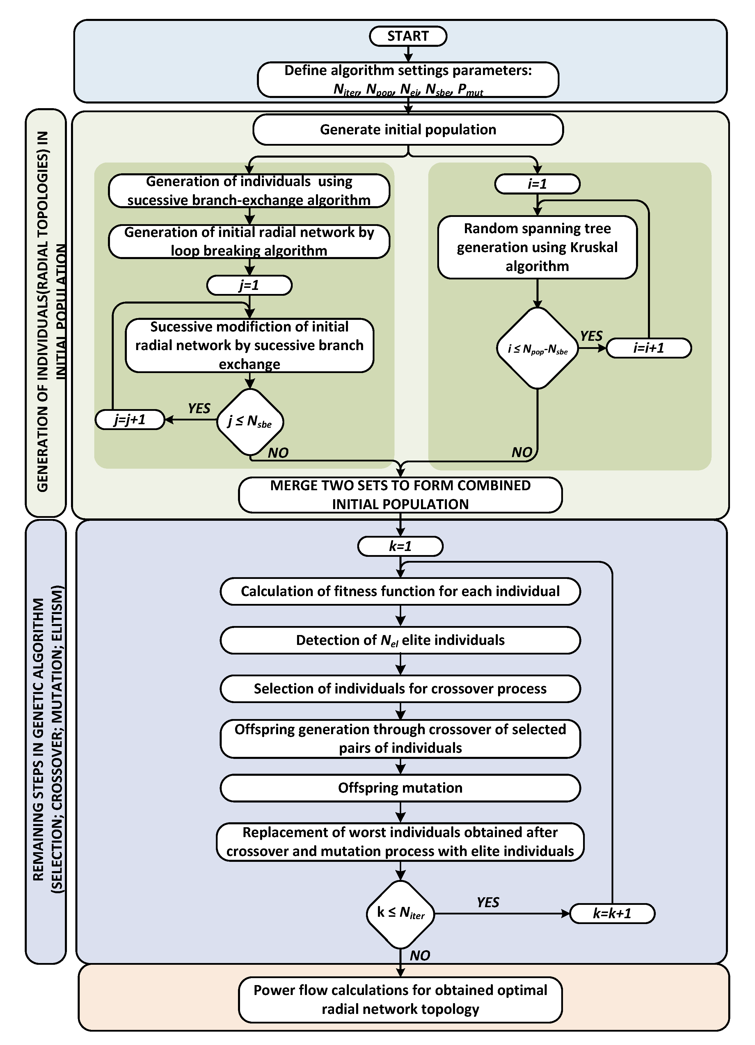
Figure 1 shows the general flowchart of the proposed methodology. The algorithm behaviour and the convergence characteristics are controlled through a set of basic parameters, as follows:
- Niter—number of evolution cycles
- Npop—population size
- Nei—number of elite individuals in each population
- Nsbe—number of individuals generated by successive branch exchange algorithm
- Pmut—mutation probability.
3. Initial Population (Feasible Radial Network Topologies) Generation
Generation of the initial population (the base set of distribution network radial topologies) is carried out by a combination of heuristic method, based on the successive branch-exchange algorithm (SBEA [3]), and a stochastic radial topology generation based on Kruskal’s algorithm [25]. This way, the initial population covers a wide range of possible solutions (search space) and we prevent the concentration of individuals in areas of local optimums. When the generation of the initial population is done only by the SBEA, the individuals who represent the solution set are restricted to a space around local optimums, so there is a risk of not detecting the global optimum. On the other side, if the generation of initial population is done exclusively by Kruskal’s algorithm we get a set of individuals (topologies), well covering the solution search space, but not landing near the global/local optimum. In this case, usually a higher number of iterations (evolution cycles) is needed to find the optimal solution.
3.1. Heuristic Method—Successive Branch-Exchange Algorithm (SBEA)
The identification of distribution network optimal radial topology is a complex and non-linear problem. To solve this complex problem, exact mathematical optimization models [13,14] or heuristic approaches [1,2,3,4] are used. One such heuristic algorithm, which avoids searching entire solution space consisting of all feasible radial topologies, is the successive branch-exchange algorithm (SBEA) [3]. The SBEA has two levels of implementation:
- ➢
- The first level determines the initial spanning tree (initial radial distribution network structure), which is further improved in the second level. The first level starts with the mashed distribution network, in which all the sectionalizing and tie switches are closed. After creating the meshed distribution network, we conduct Nel_cycles power flow calculations, each time opening the branch (or sectionalizing/tie switch) with the lowest power flow, while avoiding such operation results with isolated parts of the network or unwanted grid operating conditions. Nel_cycles represents the number of elementary cycles in the mashed distribution network, which can be calculated as:where NSP is a number of supply points.Nel_cycles = Nbr − (Nbus − NSP)The detection of the branch to be opened in each step, while avoiding isolation of a certain part of the network, can be performed by applying the Kruskal’s [25] or Prim’s [26] algorithm, for a minimum spanning tree, in which each branch has weight reversely proportional to power flow running through it. If the distribution network has multiple supply points, we can merge them into a single supply point, reducing the problem of the minimum spanning forest to the problem of a minimum spanning tree. This way, using Kruskal’s or Prim’s algorithm, we get the set of branches (the number of which is reduced in each iteration), not comprising the spanning tree, and we simply choose to open the line with the highest weight from the obtained set. Using this procedure, we sequentially switch-off Nel_cycles branches, obtaining, after this step, the initial radial fully connected distribution network. This way, we least interfere in power flows that would normally flow in mashed distribution network and assure a good power flow pattern for the initial radial distribution network, with low system losses.After this step, we get the vector containing the lists of branches (or sectionalizing/tie switches) that are offline in the initially generated radial distribution network.
- ➢
- The second level includes further improvements of the network topology obtained after the first level of SBEA. This involves the generation of a random mask vector obtained by the random shuffling of vector , indicating offline branches. For example, the shuffled vector [br60, br3, …] indicates that we first form a cycle by closing branch 60, and try to find the branch to open in a newly formed cycle that improves the objective function in the best way. If such a branch exists, we replace branch 60 with that branch in the vector containing the list of offline branches. After that, we close branch 3, and try to find the branch to open in that single newly formed cycle, in order to improve objective function, and we repeat this process according to the generated random mask vector. In this step, we use approximate equations for load flow calculations in radial distribution networks, which facilitate the generation of individuals using SBEA in a small fraction of time.Figure 2 shows the simplified distribution network with a single cycle, in which branch (b) is opened to fulfil radiality constraint. In each second loop step in SBEA, we fictively close a single branch and form a single cycle. By opening any branch in that cycle, we mainly change power flows along branches forming that cycle, with minor influence on power flows along other branches in the distribution network. If we use the approximate linearized power flows equation, we can reformulate objective functions as follows:
- Minimization of total network active power losses:The linearization of active power losses is conducted by neglecting the higher order terms related to voltages in branch power loss expressions appearing in denominator:This approximation of branch power losses is used only in population initialization to create a set of initial candidate solutions based on a heuristic approach, which uses an analytical expression derived from the linearized power loss expression to approximate loss change or loading index change in the branch exchange process. All other steps (calculation of fitness function, voltage conditions, power flows) in the algorithm use the exact full non-linear load flow expressions.
- Optimal network loading:Now, consider the branch exchange between branches b (which is originally opened) and m (which is originally closed) in Figure 2. As a result of the simplifying assumptions made above, power flow will change only in the branches, constituting the cycle shown in Figure 2. Let the branches in the cycle that extends between nodes [i, k, …, m-1, m] be denoted by the set L and the ones on the other side between nodes [i, j, … , n-1, n] by the set R.
Using simplified load flow calculations, we can approximate the power loss reduction due to branch exchange between branch b and branch m as follows:
By using an analogy between Equations (6)–(8), we can approximate the loading index reduction due to such branch exchange as follows:
To identify the optimal branch exchange, we simply use Equation (8) or (9), depending on the objective function for all branches in set L and set R and conduct branch exchange between branch b and branch, producing the highest reduction of total power losses or network loading index. If branch exchange generates an increase of system losses or loading index for all branches in set L and set R, then branch b remains offline and branch exchange is not performed. These calculations are very fast, allowing the implementation of this approach for multi-period network reconfiguration. In that case, Equations (8) and (9) transform into:
where:
- —reduction of total active energy losses due to branch exchange between branches b and m over period of time T
- —reduction of network loading index for set of time periods T due to branch exchange between branches b and m
- —active/reactive power flow through branch i for time period t
- —duration of time period t in hours
- T—set of time periods
In order to detect branches belonging to the set L and set R, after the formation of the single cycle in the network, we use the BIBC (bus injection—branch current) matrix that is often used in the load flow calculations for the radial or weekly meshed distribution networks. If we assume that the distribution network and its data is topologically sorted and the multiple supply points are represented as a single supply point, the algorithm for the formation of the BIBC matrix consists of few simple steps:
- (1)
- For the distribution system with Nbr branches and Nbus buses, start by creating a zero BIBC matrix with the dimension Nbr x Nbus.
- (2)
- If a branch brk connecting bus i and bus j does not form a cycle in the network, copy the column of the i -th bus of the BIBC matrix to the column of the j -th bus and fill a +1 to the position of the k -th row and the j -th bus column. Otherwise, if branch brk forms a cycle in the network proceed to step (3).
- (3)
- If a branch brk located between bus i and bus j forms a cycle in the network, in k-th, the column places the elements of the i-th bus column, subtracted by the j-th bus column. In addition to that, fill a +1 value to the position of the k-th row and the j-th column.
- (4)
- Repeat the procedure from step (2), until all branches are included in the BIBC matrix.
- (5)
- Using the steps described above, we can form the BIBC matrix for the mashed distribution network, in which all cycles are closed. To obtain the BIBC matrix for the radial distribution network, we can use modified Krons reduction to eliminate offline branches. This way, we obtain the BIBC matrix for the radial distribution network.
In the second level of SBEA, we close an open branch and identify a substitute branch that triggers the highest improvement of the objective function. By closing the open branch, we form a single cycle in the network, in which the branches can be divided into set R and set L, as shown in Figure 2. We can identify the branches belonging to these sets using a BIBC matrix that is formed for the radial distribution network prior to closing branch brb. To identify the branches belonging to set R and set L of the cycle that is formed after closing the branch brb (which connects bus m and bus n), we simply subtract the columns of the BIBC matrix belonging to the m-th and n-th bus. The branches having the value of 1 belong to set R, while the branches having the value of -1 belong to set L (Figure 3.). All other branches having the value 0 do not belong to the cycle which is formed after closing branch brb. The equations below demonstrate the detection of branches belonging to set R and L after the connection of br6 connected to bus 5 and bus 6 for the network shown on Figure 6 (Parent 1).
The BIBC matrix that is formed for the radial distribution network prior to closing branch brb can also be used to approximately calculate active and reactive power flows along all online branches in network (used in Equations (8)–(10)). The flowchart illustrating all steps of SBEA is shown on Figure 4.
3.2. Stochastic Method—Kruskal’s Algorithm
Kruskal’s algorithm is an algorithm used in graph theory to find a minimum spanning tree for a connected weighted graph. For any connected undirected graph, a minimal spanning tree is a subgraph of the graph that contains all vertices (buses), without any cycles in a graph, in which the total weight of edges (branches) is minimized. If the graph is not connected, then it finds a minimum spanning forest (a minimum spanning tree for each connected component).
The problem of optimal distribution network reconfiguration can be reduced to a problem of finding the spanning tree (= radial structure) that results with: minimal active power/energy losses; optimal redistribution of load in the grid, or something else depending on the defined goal function. In distribution networks with multiple supply points, the problem of optimal network reconfiguration is practically a problem of determining minimum spanning forest. However, the problem can be reduced to the problem of finding the minimum spanning tree by adequate network node renumbering and the fictional grouping of multiple supply points in a single supply point. If the initial weighted connected graph has V vertices, of which S are origins (supply points), then a minimal spanning tree has to contain the same number of vertices and V-S branches. Kruskal’s algorithm used for finding the minimum random spanning tree is implemented through the six basic steps described below:
Kruskal’s minimum random spanning tree algorithm
|
|
|
|
|
|
| If u and v don’t belong to set T: |
| Add (u,v) to T; |
| Add edge (u,v) to the set of online edges; |
| Return T and set of online edges; |
|
An illustration of the described Kruskal’s algorithm is shown in Figure 5. Instead of Kruskal’s algorithm, it is possible to use Prim’s algorithm for random spanning tree generation. Both Kruskal’s and Prim’s algorithms belong to the group of greedy algorithms, which in every step chooses what is best at that moment. Although the greedy algorithms are usually incorrect because the best at the moment does not always imply the most optimal at the end, in the case of these two algorithms, specific properties guarantee the provision of the correct results.
4. Adaption of Other Steps in Genetic Algorithm
4.1. Fitness Function Calculation and Separation of Elite Individuals
The fitness function value is calculated for every individual in the population using the following equation:
where fitness(i) is fitness function for ith individual in population.
Single period or Multi-period
This way, both minimization of total network losses and network loading index are transformed to maximization of fitness function, given that individuals that have the highest total power losses (loading index) have the lowest fitness function.
After the calculation of fitness function for every individual, the Nel elite individuals from the population are identified. These elite individuals are allowed to pass directly to the next evolution epoch unchanged, but can also participate as parents in the crossover process if they are selected. During the selection process, the parent pairs, which participate in the crossover process, are chosen. The fitness proportionate selection, also known as the roulette wheel selection, is used for the selection of parent pairs. The individuals with lower fitness function have a lower probability of being selected as parents in the crossover process. Every individual within the population has respective probability of selection p(i), according to the equation below:
Based on each individual selection probability p(i), the cumulative probability f(i) for each individual is obtained according to the following equation:
The further process involves the generation of two random numbers in [0, 1] interval and the selection of two parents for reproduction process. Individual ‘i’ enters the parent pair if the generated random number ‘r’ is within interval . This process is repeated until Npop/2 parent pairs are created.
4.2. Crossover Process
From every pair of parents two new offspring are created, which need to keep the part of the parent’s genetic material, preferably the best one. In most of the approaches that employ evolution algorithms for the network reconfiguration problem, this is usually the point at which the problems appear [5,8,10,11,16,17,19,20,22]. These problems are related to the methods used in the crossover process, which result in offspring that violate radiality constraint or have isolated parts of the network. Given that, the offspring are usually further analysed and corrected to impose radiality and connectivity constraints. In addition to prolonging execution time and slowing down the convergence rate, these correction algorithms usually significantly change offspring so that they no longer resemble and contain the best genetic material from their parents. Given this, we introduce the improved approach, which deals with and eliminates these problems.
An illustration of the crossover process that we propose is shown on Figure 6. During the crossover process, we find an intersection and union of online branches included in both of the parents. The process of obtaining children is based on a subgraph that is made from the union of online branches of both parents, to which we assign weight in specific manner. Zero weight is assigned to all online branches that belong to the parent online branch intersection. Other branches that are present in union of online parent branches are assigned random weights. Applying Kruskal’s or Prim’s algorithm on a weighted subgraph created in such a way, we obtain a single offspring. To obtain two offspring, we repeat this process by refreshing random weights assigned to the branches that are not members of parents’ online branch intersection. Using this method of crossover, all ‘good’ genetic material is imprinted in children. Children contain all branches that appear in both parents and part of branches that make difference between parents. Offspring obtained in this way are guaranteed to fulfil the radiality and connectivity constraints without the need for further offspring rechecking or corrections.
4.3. Mutation Process
After the finalization of the crossover process, we enter a mutation phase. In the classical approaches, in this phase similar problems to the ones in crossover phase appear. These problems are related to the violation of the radiality and connectivity constraints after the mutation operator is applied on the offspring. The offspring undergoes the mutation process if the randomly generated number in interval [0, 1], for that individual, is lower or equal to the mutation probability Pmut.
In this paper, we propose the additional enhancements of this step, which solve these issues. An illustration of the mutation process based on Kruskal’s algorithm is shown in Figure 7. The mutation process consists of the random insertion/activation of a single offline branch. This action creates a single cycle in the distribution network. To eliminate this cycle, random weight is associated with each online branch and Kruskal’s or Prim’s algorithm is applied to obtain the radial connected network topology. Alternatively, the BIBC matrix associated with the state prior to the insertion/activation of single offline branch can be used to identify the branches belonging to the newly formed cycle (as described in Section 3.1), and we can than randomly choose one branch from this set to switch off.
The mutation process can be improved even further if SBEA is introduced in this process. This way, using Equations (8)–(11), depending on the objective function, we can improve the network topology through the mutation process. Both approaches guarantee that the individual mutated in this way will fulfil radiality and connectivity constraints without the need for further rechecking or corrections.
4.4. Elitism
Elitism is a process which is introduced to enable the best individuals to participate unchanged in the next evolution epoch. This means that Nei individuals with the lowest fitness function values are substituted with the same number of parents that have the highest fitness function. An illustration of this process is shown on Figure 8.
After inserting elite individuals into the population, the previously described steps of the genetic algorithm are repeated until the pre-defined number of iterations is reached or the defined convergence criteria is met.
5. Case Study
The proposed algorithm was implemented in Matlab and all tests were performed on a Windows machine equipped with an AMD six-core (3.3 GHz) processor and 8 GB of RAM. To test the effectiveness and algorithm convergence rate, three standard test networks of different sizes and topology complexity were considered:
- Network I—33 bus: The test system is a hypothetical 12.66 kV system with a single supply point, 33 busses and 5 elementary cycles (tie lines). The system data is given in [3], and this system is usually referred to as “Baran’s test case”. The total system load equals 5084.26 kW and 2547.32 kVAr. For the base case network topology, the total system losses equal to 210.99 kW. With the application of the proposed algorithm, the total system losses were reduced to 139.2 kW, which represents a 34.03% loss reduction in relation to the base case topology.
- Network II—1760 bus: The test system is a 130.8 kV system with 14 supply points, 1760 buses and 54 elementary cycles. The system data is given in [27]. The total system load equals 249.73 MW and 148.72 MVAr. For the base case network topology, the total system losses equal to 2.992 MW. With the application of the proposed algorithm, the total system losses were reduced to 914.02 kW, which represents a 69.46% loss reduction, in relation to the base case topology.
- Network III—4400_50 bus: The test system is a 130.8 kV system with 35 supply points, 4400 buses and 185 elementary cycles. The system data is given in [27]. The total system load equals 624.34 MW and 371.80 MVAr. The total system losses for the initial network topology is equal to 7.481 MW. With the application of the proposed algorithm, the total system losses were reduced to 1.9 kW, which represents a 74.6% loss reduction, in relation to the initial network topology.
For all test networks, the minimum allowed voltage is 0.9 p.u. and maximum allowed voltage is 1.1 p.u. The summary of test network data is given in Table 1.
To test the validity and effectiveness of the proposed approach, the results were compared to the MIQP, MIQCP and MISOCP distribution network reconfiguration approaches presented in [13], as well as the reported global optimum solutions obtained using the approach presented in [12]. The MIQP, MIQCP and MISOCP models were formed using GAMS modelling language and solved using CPLEX solver.
We can see from Table 2 that the proposed hybrid heuristic genetic algorithm has a computational time comparable to convex models (MIQP, MIQCP and MISOCP) for small distribution network models and a much faster convergence rate for larger network models. We assume that the method converged if we obtain global optimum solution in three consecutive evaluation epochs. The results related to the proposed hybrid heuristic genetic algorithm are obtained with the same setup parameters: population size: = 14, mutation probability: = 2%, number of individuals in the initial population generated using SBEA: = 4 and the number of elite individuals: = 1.
The convergence rates for different test networks are shown in Figure 9. The figure shows the reported global optimum and evolution of the average and minimum fitness value in the whole population.
The decrease of the population minimum fitness value in consecutive evolution epochs is a result of the mutation process, which happened in that evolution epoch, decreasing the fitness function for some individuals. Despite this, we see the rapid improvement of the population average fitness value and the strive of individuals toward the optimal solution. If we compare general parameters for the genetic algorithm used in this analysis (population size:=14, number of epochs:=20) to the parameters used in other similar approaches based on genetic algorithm, we can see that we used a much lower population size and number of iterations to detect optimal solution. This doesn’t interfere with solution quality, nor does it result in solution dispersion. For all networks, network reconfiguration was performed repeatedly, always landing with the same best solution. This improved convergence characteristic is a result of a special adjustment, introduced in the process of initial population generation, crossover and the mutation process, which were described in detail in previous sections. In addition to this, the proposed solution approach is suitable for the parallelization on multicore CPU, giving the opportunity for even shorter computational times.
Figure 10 shows the network voltage profile before and after network reconfiguration for the 1760 and 4400_50 bus network. Although the primary objective was network active power loss minimization, network reconfiguration provided topology with a more balanced voltage profile in relation to starting network topology. These positive effects of network reconfiguration on voltage conditions are evident, both for the 1760 and 4400_50 bus network. Given that the 1760 and 4400_50 bus network share topological similarities (both were derived by replicating the 880 bus network and adding additional tie lines), a similar voltage improvement is evident in both cases. A relatively wide voltage profile, characteristic for initial topology (1.0–0.956 p.u.), is indirectly reduced through network reconfiguration to range (1.0–0.991 p.u.), with bus voltages very close to nominal values and more homogeneous voltage profile distribution.
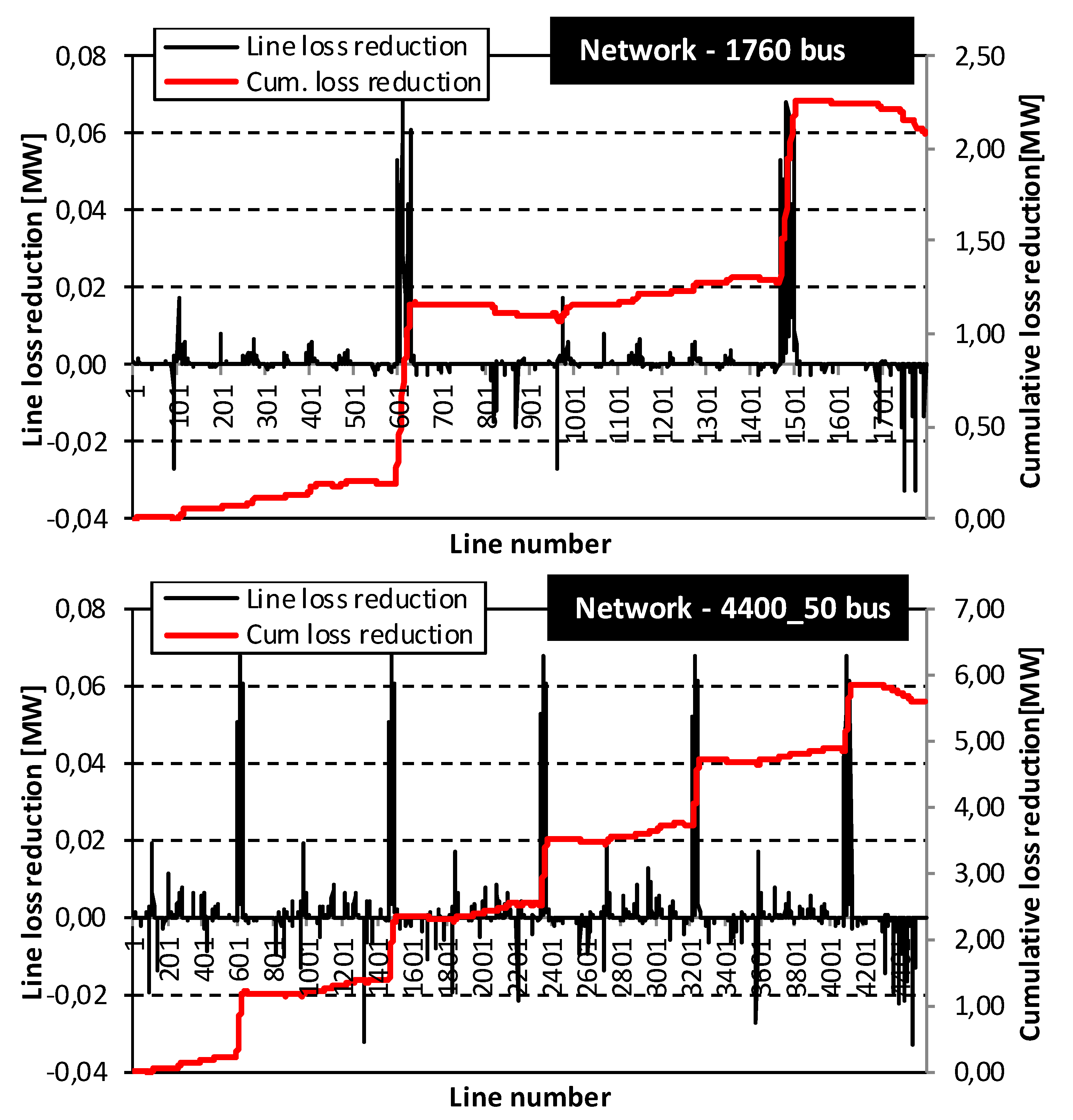
Figure 11 shows the decrease/increase of the line active power losses for the optimal network topology in relation to the initial network topology for the 1760 and 4400_50 bus networks. From Figure 11, we can see the cumulative decrease of active power losses in the amount of 2.078MW for the 1760 bus network and in the amount of 5.581 MW for the 4400_50 bus network, in relation to the initial network topology. This represents a 69.5% (for 1760 bus network) and 74.6% (for 4400_50 bus network) decrease of active power losses in relation to the initial network topology.
6. Conclusions
In this paper, a novel hybrid heuristic-genetic algorithm for the optimal distribution network reconfiguration under normal system operating conditions is proposed. The main issues related to the application of genetic algorithms to this type of optimization problems are related to the generation of a large amount of unfeasible solutions (that violate radiality and connectivity constraint), which are created in the crossover and mutation process. This requires constant rechecking and the implementation of heuristic correction algorithms on offspring, which significantly affects the algorithm efficiency. In addition to that, such correction processes usually significantly change the offspring structure and limit the transfer of good genetic material from parents to the children, slowing down the convergence rate. Additionally, in these approaches, the generation of the initial population is usually not very effective.
The algorithm proposed in this paper solves these issues and assures convergence in a short execution time. Due to these enhancements, it is possible to apply the proposed algorithm on large scale distribution networks with realistic topology complexity, which was shown in the case study. Additionally, the algorithm structure gives the opportunity for parallel implementation, which could improve calculation speed even further. The algorithm is general and can be used to minimize the total network losses, as well as to minimize network element loading. Generation of initial population by the combination of a heuristic approach based on SBEA and a stochastic approach based on the Kruskal algorithm effectively covers the solution of space and provides good starting points, which produce global optimums in only a few iterations. The comparative tests performed on some tests systems have demonstrated the computational effectiveness of the proposed method, as well as accuracy in detecting the global optimum solution. These positive aspects are especially pronounced on large distribution networks. Due to a fast convergence rate, the algorithm can be applied for multi-period distribution network reconfiguration, to minimize network energy losses, or to optimally balance network loading over a larger time span.
Author Contributions
D.J. and R.Č. defined the main concepts and implemented the proposed algorithms. P.S. and J.V. participated in the simulation part and the case study analysis. All authors have read and agreed to the published version of the manuscript.
Funding
This research has been funded with support from the European Commission under the project Green-Tech-WB: Smart and Green technologies for innovative and sustainable societies in the Western Balkans (551984-EM-1-2014-1-ES-ERA MUNDUS-EMA2).
Conflicts of Interest
The authors declare no conflict of interest.
References
- Civanlar, S.; Grainger, J.J.; Yin, H.; Lee, S.S.H. Distribution feeder reconfiguration for loss reduction. IEEE Trans. Power Deliv. 1988, 3, 1217–1223. [Google Scholar] [CrossRef]
- Abul’Wafa, A.R. A new heuristic approach for optimal reconfiguration in distribution systems. Electr. Power Syst. Res. 2011, 81, 282–289. [Google Scholar] [CrossRef]
- Baran, M.E.; Wu, F.F. Network reconfiguration in distribution systems for loss reduction and load balancing. IEEE Trans. Power Deliv. 1989, 4, 1401–1407. [Google Scholar] [CrossRef]
- Rosseti, G.J.S.; de Oliveira, E.J.; de Oliveira, L.W.; Silva, I.C.; Peres, W. Optimal allocation of distributed generation with reconfiguration in electric distribution systems. Electr. Power Syst. Res. 2013, 103, 178–183. [Google Scholar] [CrossRef]
- Bahadoorsingh, S.; Milanović, J.V.; Zhang, Y.; Gupta, C.P.; Dragovic, J. Minimization of voltage sag costs by optimal reconfiguration of distribution network Using genetic algorithms. IEEE Trans. Power Deliv. 2007, 22, 2271–2278. [Google Scholar] [CrossRef]
- Kashem, M.A.; Ganapathy, V.; Jasmon, G.B. Network reconfiguration for enhancement of voltage stability in distribution networks. IEE Proc. Gener. Transm. Distrib. 2000, 147, 171. [Google Scholar] [CrossRef] [Green Version]
- Arun, M.; Aravindhababu, P. A new reconfiguration scheme for voltage stability enhancement of radial distribution systems. Energy Convers. Manag. 2009, 50, 2148–2151. [Google Scholar] [CrossRef]
- Zou, B.C.; Gong, Q.W.; Li, X.; Chen, D.J. Reconfiguration in distribution systems based on refined genetic algorithm for improving voltage quality. In Proceedings of the 2011 Asia-Pacific Power and Energy Engineering Conference, Wuhan, China, 25–28 March 2011; pp. 1–4. [Google Scholar]
- Roytelman, I.; Melnik, V.; Lee, S.S.H.; Lugtu, R.L. Multi-objective feeder reconfiguration by distribution management system. IEEE Trans. Power Syst. 1996, 11, 661–667. [Google Scholar] [CrossRef]
- Montoya, D.P.; Ramirez, J.M.; Zuluaga, J.R. Multi-objective optimization for reconfiguration and capacitor allocation in distribution systems. In Proceedings of the 2014 North American Power Symposium (NAPS), Pullman, WA, USA, 7–9 September 2014; pp. 1–6. [Google Scholar]
- Tomoiagă, B.; Chindriş, M.; Sumper, A.; Sudria-Andreu, A.; Villafafila-Robles, R. Pareto optimal reconfiguration of power distribution systems using a genetic algorithm based on NSGA-II. Energies 2013, 6, 1439–1455. [Google Scholar] [CrossRef] [Green Version]
- Morton, A.B.; Mareels, I.M.Y. An efficient brute-force solution to the network reconfiguration problem. IEEE Trans. Power Deliv. 2000, 15, 996–1000. [Google Scholar] [CrossRef]
- Taylor, J.A.; Hover, F.S. Convex models of distribution system reconfiguration. IEEE Trans. Power Syst. 2012, 27, 1407–1413. [Google Scholar] [CrossRef]
- Llorens-Iborra, F.; Riquelme-Santos, J.; Romero-Ramos, E. Mixed-integer linear programming model for solving reconfiguration problems in large-scale distribution systems. Electr. Power Syst. Res. 2012, 88, 137–145. [Google Scholar] [CrossRef]
- Abdelaziz, M. Distribution network reconfiguration using a genetic algorithm with varying population size. Electr. Power Syst. Res. 2017, 142, 9–11. [Google Scholar] [CrossRef]
- Chen, J.; Zhang, F.; Zhang, Y. Distribution network reconfiguration based on simulated annealing immune algorithm. Energy Procedia 2011, 12, 271–277. [Google Scholar] [CrossRef] [Green Version]
- Tomoiagă, B.; Chindriş, M.; Sumper, A.; Villafafila-Robles, R.; Sudria-Andreu, A. Distribution system reconfiguration using genetic algorithm based on connected graphs. Electr. Power Syst. Res. 2013, 104, 216–225. [Google Scholar] [CrossRef]
- Queiroz, L.M.O.; Lyra, C. Adaptive hybrid genetic algorithm for technical loss reduction in distribution networks under variable demands. IEEE Trans. Power Syst. 2009, 24, 445–453. [Google Scholar] [CrossRef]
- Alemohammad, S.H.; Mashhour, E.; Saniei, M. A market-based method for reconfiguration of distribution network. Electr. Power Syst. Res. 2015, 125, 15–22. [Google Scholar] [CrossRef]
- Tahboub, A.M.; Pandi, V.R.; Zeineldin, H.H. Distribution system reconfiguration for annual energy loss reduction considering variable distributed generation profiles. IEEE Trans. Power Deliv. 2015, 30, 1677–1685. [Google Scholar] [CrossRef]
- Montoya, D.P.; Ramirez, J.M.; Theory, A.G. A minimal spanning tree algorithm for distribution networks configuration. In Proceedings of the 2012 IEEE Power and Energy Society General Meeting, San Diego, CA, USA, 22–26 July 2012; pp. 1–7. [Google Scholar]
- Wu, O.; Cheng, H.; Zhang, X.; Yao, L.; Bazargan, M. Random Spanning Tree Based Improved GA for Distribution Reconfiguration. In Proceedings of the 2009 Asia-Pacific Power and Energy Engineering Conference, Wuhan, China, 27–31 March 2009; pp. 1–4. [Google Scholar]
- Zhang, J.; Yuan, X.; Yuan, Y. A novel genetic algorithm based on all spanning trees of undirected graph for distribution network reconfiguration. J. Mod. Power Syst. Clean Energy 2014, 2, 143–149. [Google Scholar] [CrossRef] [Green Version]
- Swarnkar, A.; Gupta, N.; Niazi, K.R. A novel codification for meta-heuristic techniques used in distribution network reconfiguration. Electr. Power Syst. Res. 2011, 81, 1619–1626. [Google Scholar] [CrossRef]
- Kruskal, J.B. On the shortest spanning subtree of a graph and the traveling salesman problem. Proc. Am. Math. Soc. 1956, 7, 48–50. [Google Scholar] [CrossRef]
- Prim, R.C. Shortest connection networks and some generalizations. Bell Syst. Tech. J. 1957, 36, 1389–1401. [Google Scholar] [CrossRef]
- Distribution Feeder Reconfiguration (DFR) Test Cases. Available online: http://roberge.segfaults.net/joomla/index.php/dfr (accessed on 15 March 2020).
Figure 1.
Flowchart of the proposed hybrid heuristic-genetic algorithm used to solve optimal reconfiguration problem.
Figure 1.
Flowchart of the proposed hybrid heuristic-genetic algorithm used to solve optimal reconfiguration problem.

Figure 2.
Simplified distribution network with single opened cycle.
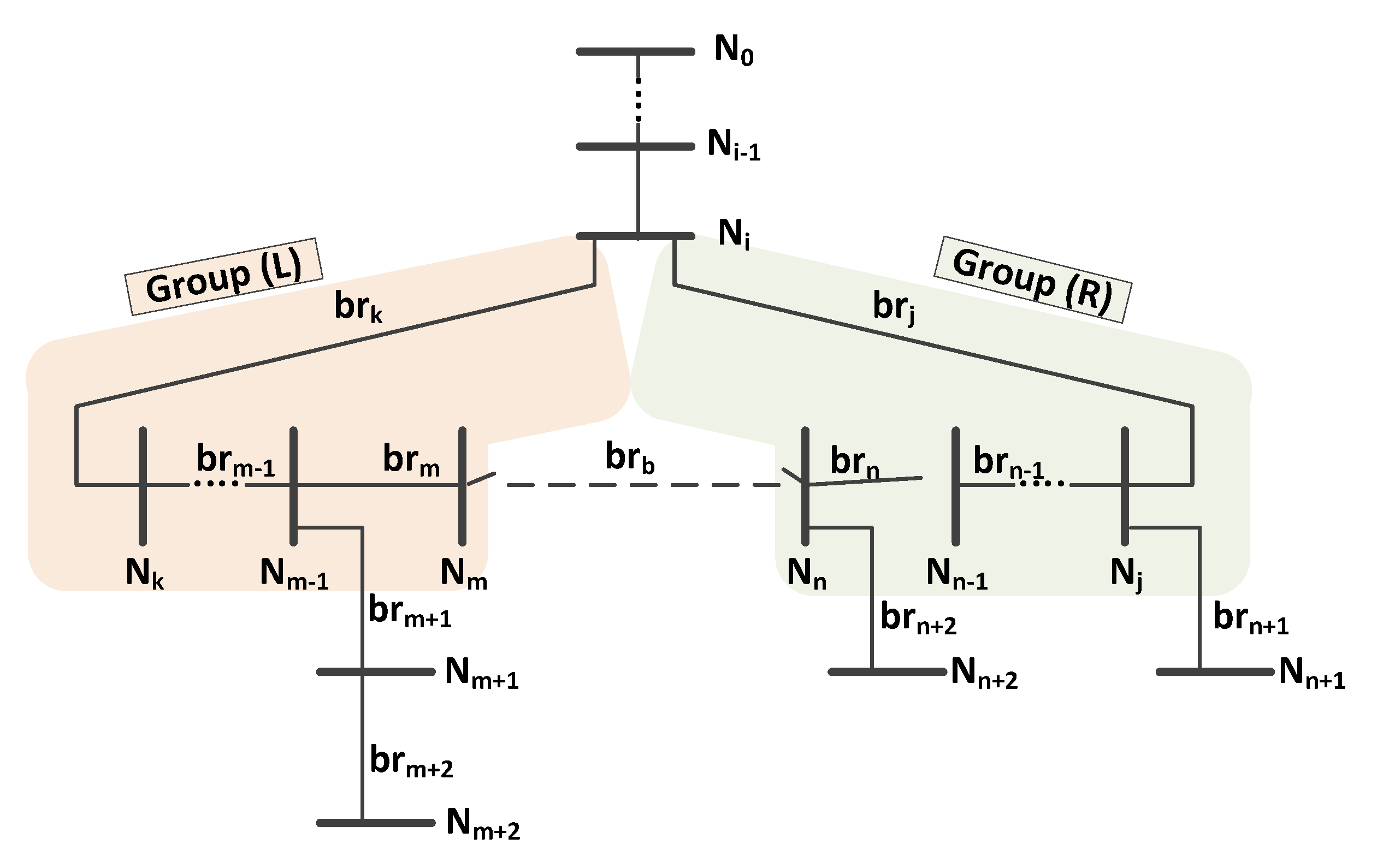
Figure 3.
Cycle detection and portioning based on BIBC matrix.
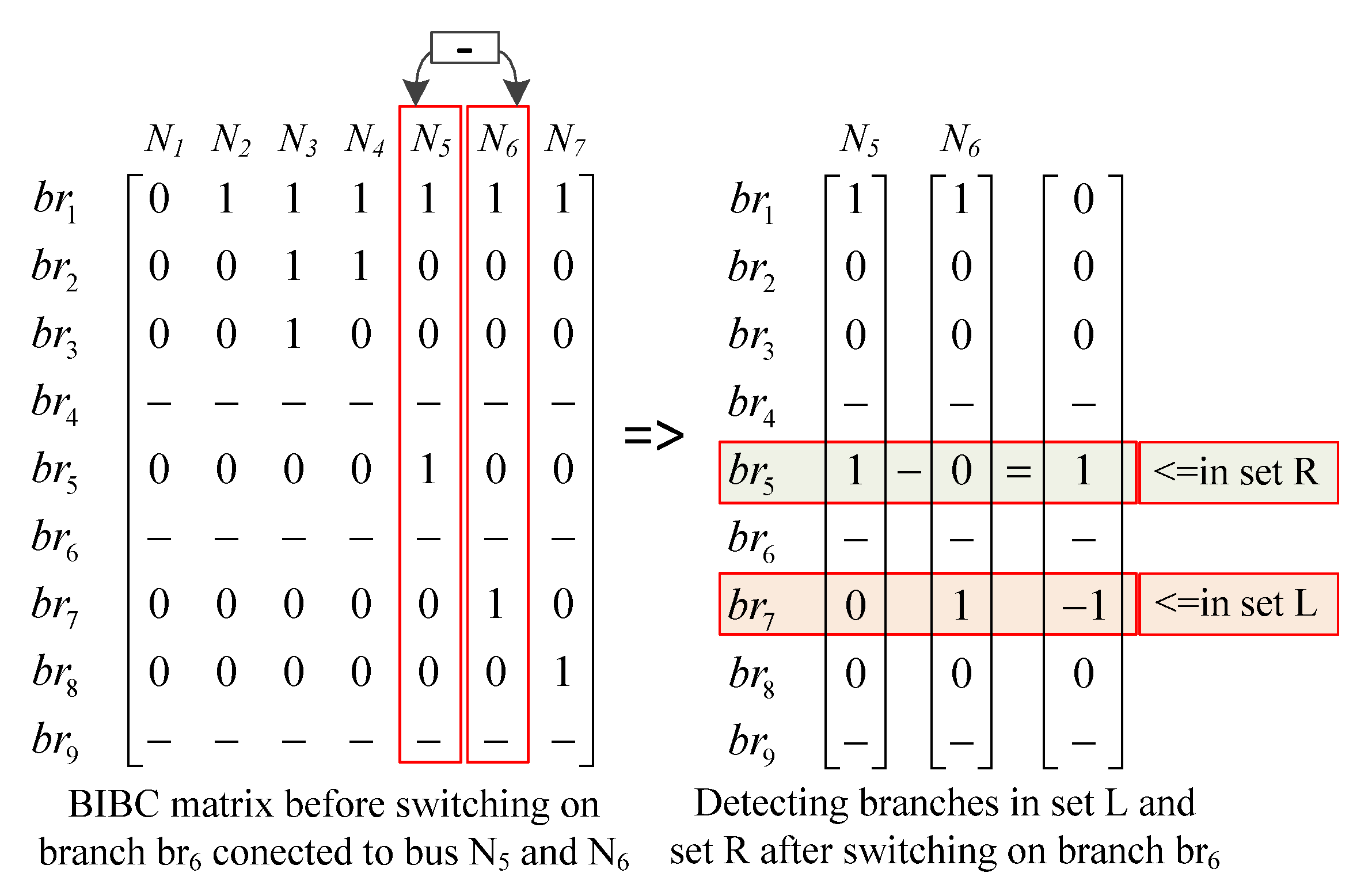
Figure 4.
Flowchart of SBEA.
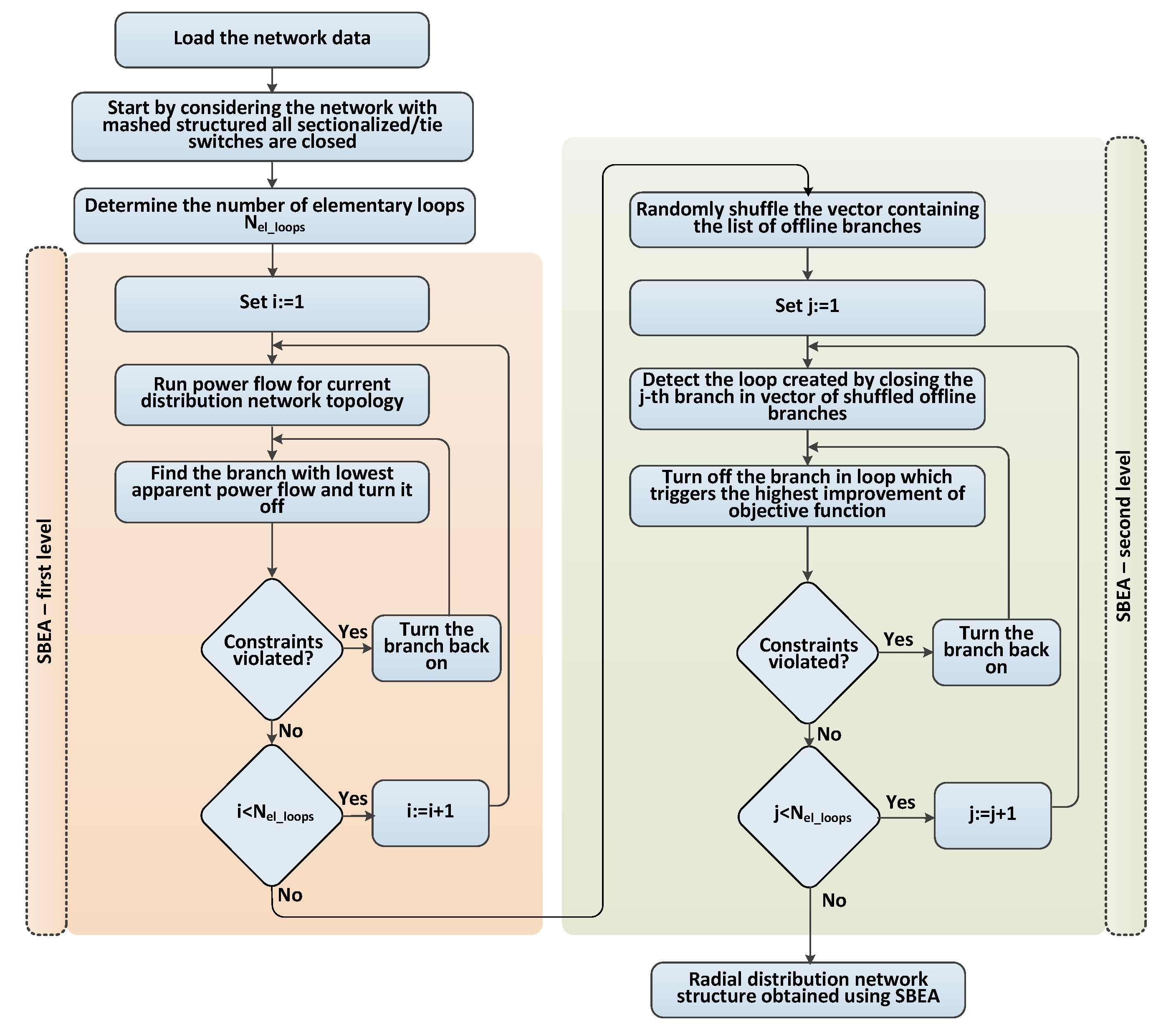
Figure 5.
Generation of random radial distribution network topology using Kruskal’s algorithm.
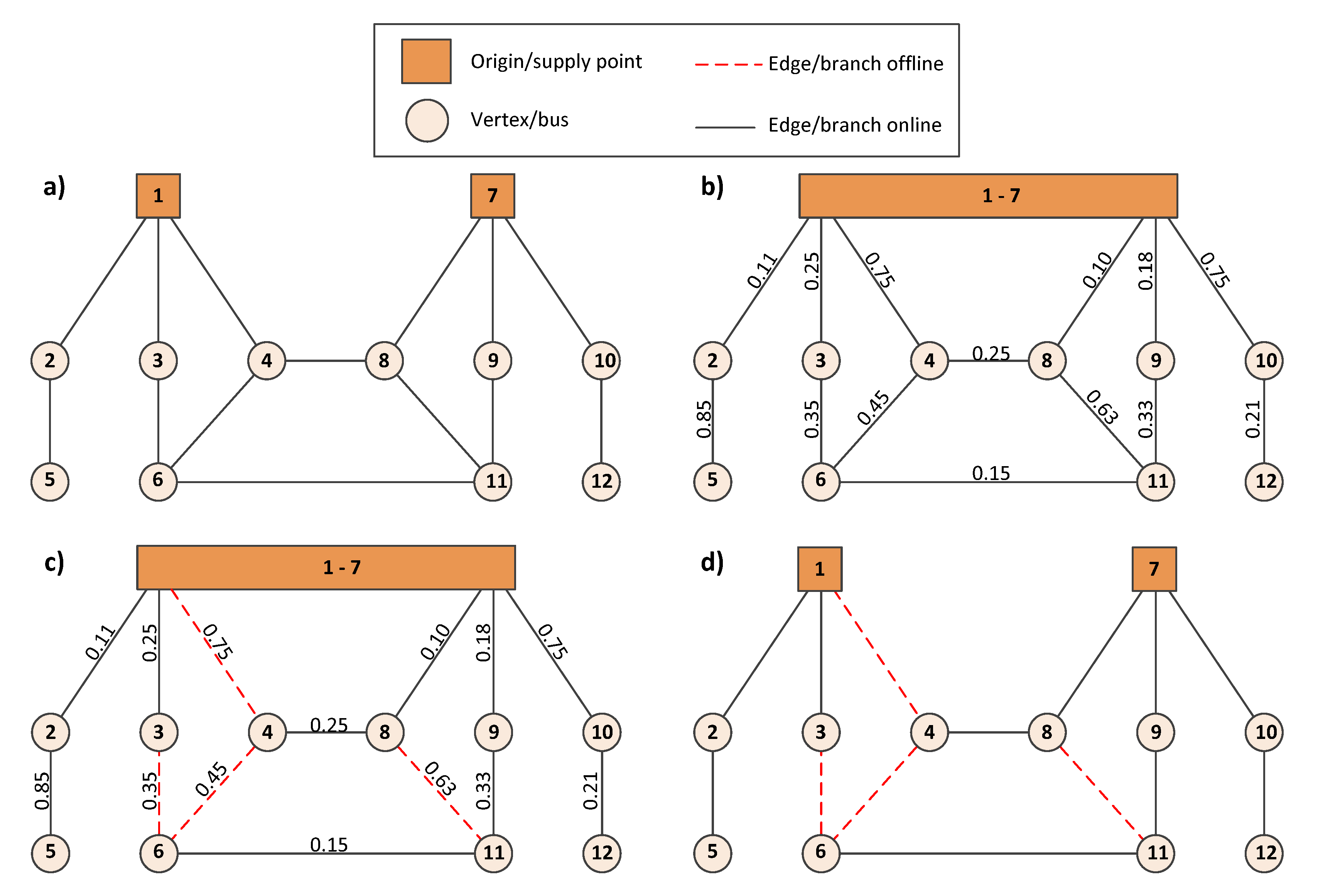
Figure 6.
Illustration of the proposed crossover process.
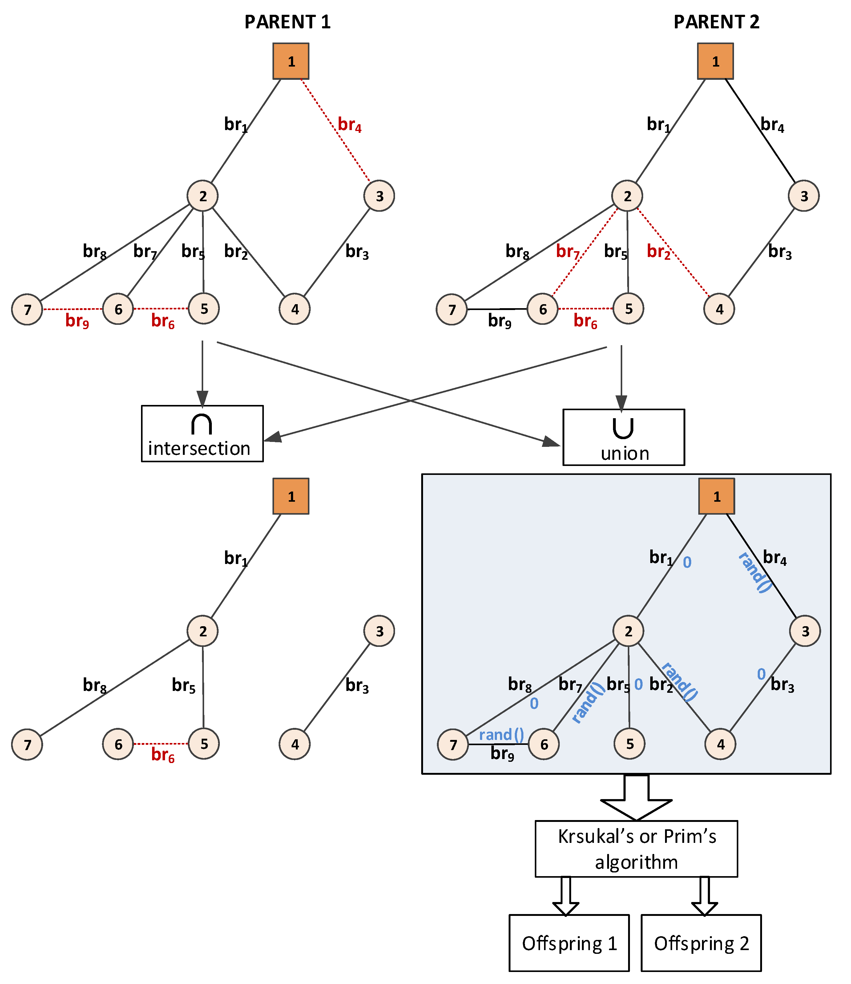
Figure 7.
Illustration of mutation process.
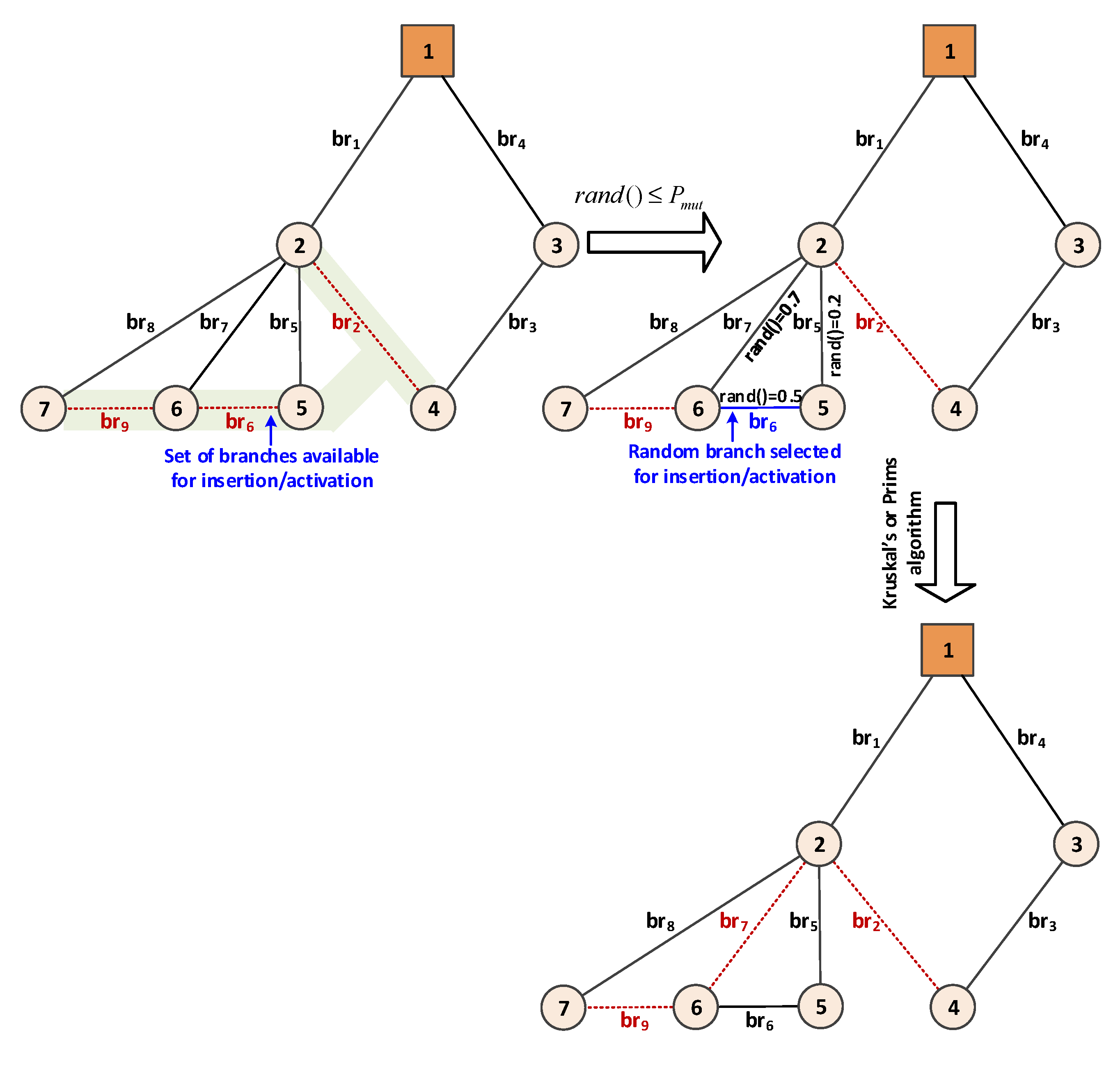
Figure 8.
Illustration of elitism.
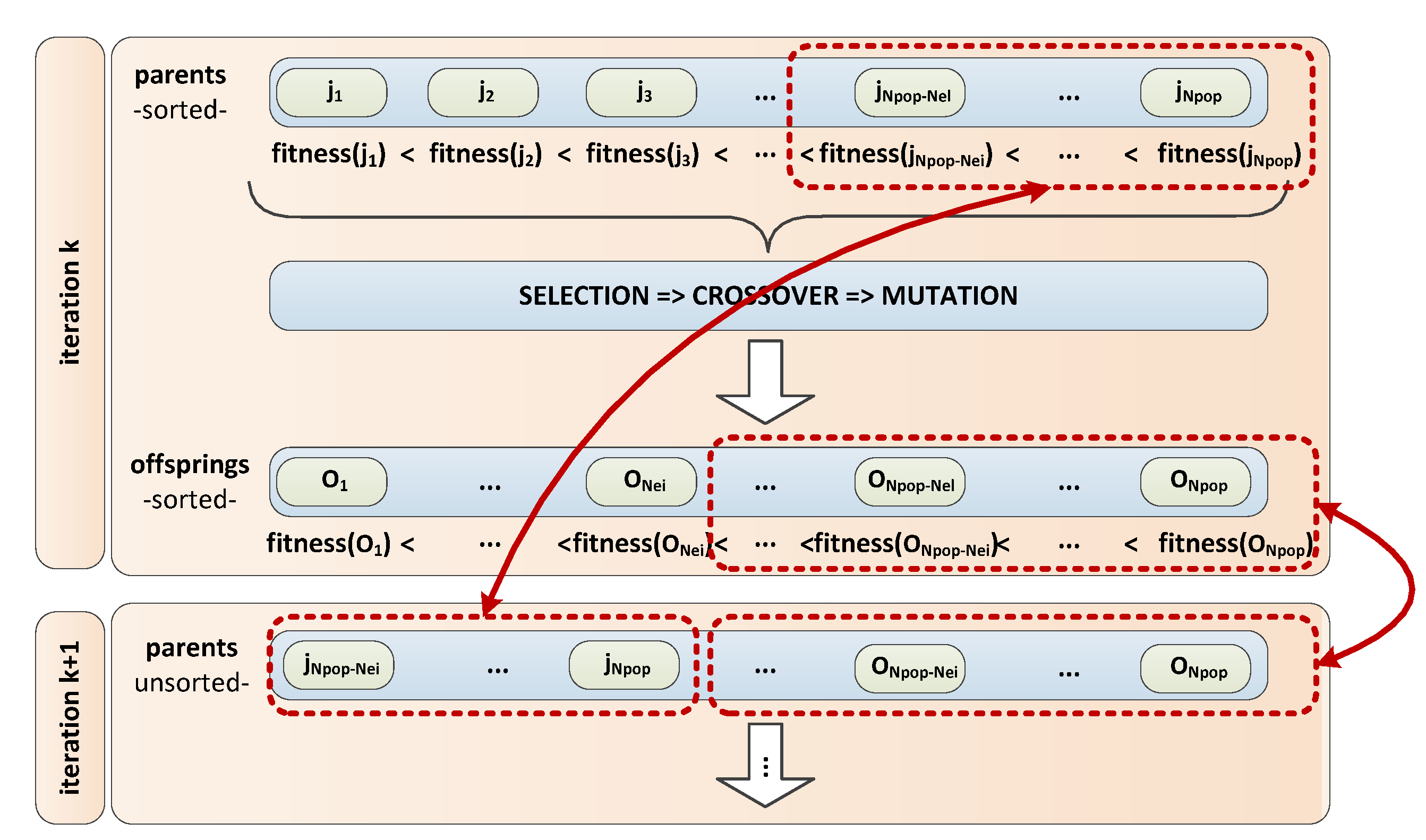
Figure 9.
Computation time for different test networks.
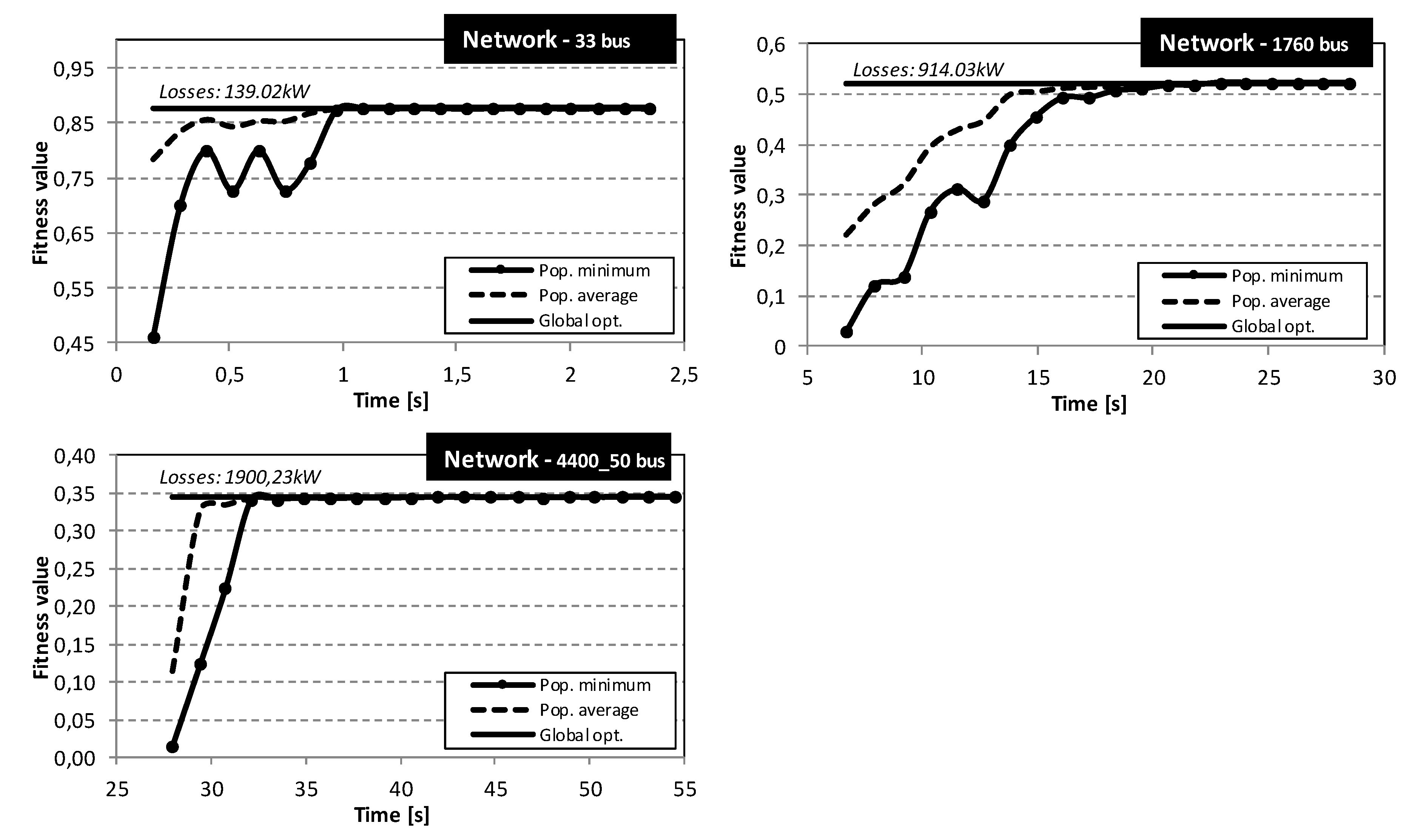
Figure 10.
Voltage profile for initial and optimal network topology (for 1760 and 4400_50 bus network).
Figure 10.
Voltage profile for initial and optimal network topology (for 1760 and 4400_50 bus network).
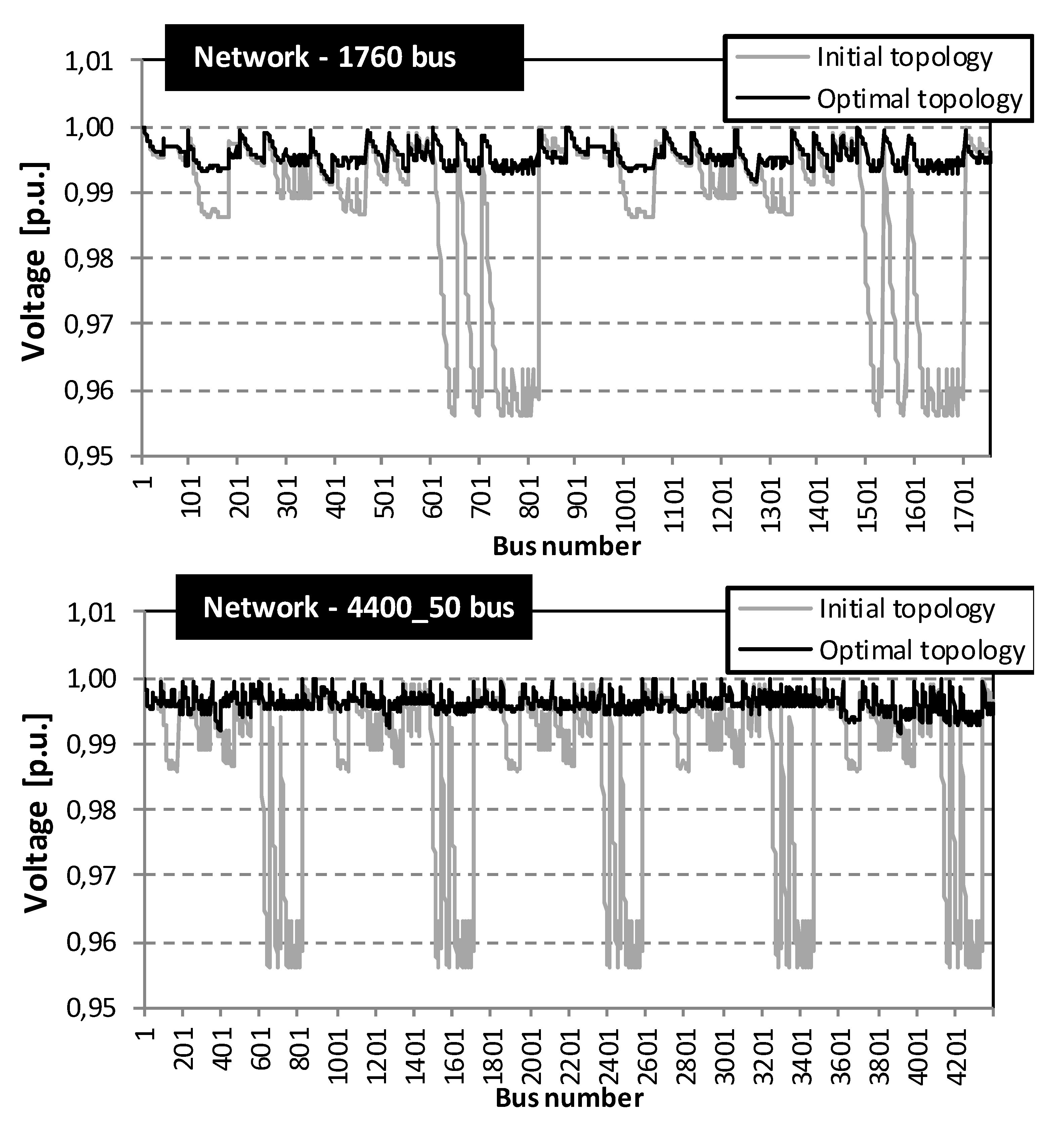
Figure 11.
Line active power loss reduction (for 1760 and 4400_50 bus network).

Table 1.
Test networks—data summary.
| Buses (Nbus) | Supply Points (NSP) | Lines (Nbr) | Sectionalizing Switches | Tie Switches | Initial Losses (kW) |
|---|---|---|---|---|---|
| 33 | 1 | 37 | 32 | 5 | 210.99 |
| 1760 | 14 | 1800 | 1746 | 54 | 2992.00 |
| 4400_50 | 35 | 4550 | 4365 | 185 | 7481.70 |
Table 2.
Computational results for different test networks.
| Test Network | Losses (Kw) | Losses Reduction (%) | Computational Time(s) | |||
|---|---|---|---|---|---|---|
| Hybrid Heur.-Gen. | MIQP | MIQCP | MISOCP | |||
| Offline Branches | ||||||
| Network I (33bus) | 139.2 | 34.03% | 0.396 | 0.57 (r.g. = 2%) | 2.14 (r.g. = 2%) | 2.801 (r.g. = 2%) |
| 7; 9; 14; 32; 37 | ||||||
| Network II (1760bus) | 914.1 | 69.46% | 9.18 | >36,000 (r.g. = 2%) | >36,000 (r.g. = 2%) | >36,000 (r.g. = 2%) |
| 84; 130; 141; 159; 190; 282; 288; 306; 312; 409; 411; 452; 494; 596; 616; 630; 631; 637; 698; 815; 844; 957; 1003; 1014; 1032; 1063; 1155; 1161; 1179; 1185; 1282; 1284; 1325; 1367; 1469; 1489; 1503; 1504; 1510; 1571; 1688; 1717; 1758; 1761; 1762; 1763; 1769; 1773; 1785; 1788; 1789; 1790; 1796; 1800 | ||||||
| Network III (4400_50bus) | 1900.2 | 74.60% | 30.77 | >36,000 (r.g. = 2%) | >36,000 (r.g. = 2%) | >36,000 (r.g. = 2%) |
| 81; 84; 117; 136; 168; 190; 232; 239; 282; 284; 288; 334; 399; 406; 424; 434; 447; 453; 494; 558; 613; 616; 627; 634; 639; 645; 647; 794; 812; 843; 916; 953; 958; 992; 1003; 1018; 1041; 1062; 1101; 1113; 1154; 1158; 1179; 1184; 1187; 1198; 1280; 1283; 1307; 1357; 1427; 1466; 1485; 1501; 1504; 1509; 1513; 1518; 1571; 1667; 1691; 1716; 1730; 1744; 1794; 1829; 1865; 1880; 1919; 1961; 1990; 2028; 2032; 2052; 2071; 2076; 2089; 2129; 2152; 2162; 2190; 2198; 2204; 2237; 2241; 2300; 2305; 2341; 2360; 2361; 2374; 2378; 2382; 2385; 2394; 2427; 2444; 2564; 2590; 2609; 2693; 2742; 2752; 2762; 2786; 2811; 2860; 2897; 2907; 2925; 2931; 2934; 3000; 3012; 3028; 3030; 3066; 3069; 3076; 3110; 3115; 3193; 3198; 3215; 3232; 3240; 3249; 3261; 3265; 3268; 3309; 3431; 3463; 3576; 3622; 3633; 3651; 3682; 3774; 3780; 3798; 3804; 3901; 3903; 3944; 3986; 4088; 4108; 4122; 4123; 4129; 4190; 4307; 4336; 4377; 4378; 4383; 4385; 4392; 4407; 4411; 4419; 4421; 4435; 4446; 4450; 4473; 4485; 4488; 4489; 4490; 4496; 4500; 4506; 4513; 4520; 4523; 4524; 4527; 4528; 4530; 4537; 4539; 4541; 4550; | ||||||
© 2020 by the authors. Licensee MDPI, Basel, Switzerland. This article is an open access article distributed under the terms and conditions of the Creative Commons Attribution (CC BY) license (http://creativecommons.org/licenses/by/4.0/).
Share and Cite
MDPI and ACS Style
Jakus, D.; Čađenović, R.; Vasilj, J.; Sarajčev, P. Optimal Reconfiguration of Distribution Networks Using Hybrid Heuristic-Genetic Algorithm. Energies 2020, 13, 1544. https://doi.org/10.3390/en13071544
AMA Style
Jakus D, Čađenović R, Vasilj J, Sarajčev P. Optimal Reconfiguration of Distribution Networks Using Hybrid Heuristic-Genetic Algorithm. Energies. 2020; 13(7):1544. https://doi.org/10.3390/en13071544
Chicago/Turabian StyleJakus, Damir, Rade Čađenović, Josip Vasilj, and Petar Sarajčev. 2020. "Optimal Reconfiguration of Distribution Networks Using Hybrid Heuristic-Genetic Algorithm" Energies 13, no. 7: 1544. https://doi.org/10.3390/en13071544
Note that from the first issue of 2016, this journal uses article numbers instead of page numbers. See further details here.