Primary Production, an Index of Climate Change in the Ocean: Satellite-Based Estimates over Two Decades

Abstract

Primary production by marine phytoplankton is one of the largest fluxes of carbon on our planet. In the past few decades, considerable progress has been made in estimating global primary production at high spatial and temporal scales by combining in situ measurements of primary production with remote-sensing observations of phytoplankton biomass. One of the major challenges in this approach lies in the assignment of the appropriate model parameters that define the photosynthetic response of phytoplankton to the light field. In the present study, a global database of in situ measurements of photosynthesis versus irradiance (P-I) parameters and a 20-year record of climate quality satellite observations were used to assess global primary production and its variability with seasons and locations as well as between years. In addition, the sensitivity of the computed primary production to potential changes in the photosynthetic response of phytoplankton cells under changing environmental conditions was investigated. Global annual primary production varied from 48.7 to 52.5 Gt C yr⁻¹ over the period of 1998–2018. Inter-annual changes in global primary production did not follow a linear trend and regional differences in the magnitude and direction of change in primary production were observed. Trends in primary production followed directly from changes in chlorophyll-a and were related to changes in the physico-chemical conditions of the water column due to inter-annual and multi-decadal climate oscillations. Moreover, the sensitivity analysis in which P-I parameters were adjusted by ±1 standard deviation showed the importance of accurately assigning photosynthetic parameters in global and regional calculations of primary production. The assimilation number of the P-I curve showed strong relationships with environmental variables such as temperature and had a practically one-to-one relationship with the magnitude of change in primary production. In the future, such empirical relationships could potentially be used for a more dynamic assignment of photosynthetic rates in the estimation of global primary production. Relationships between the initial slope of the P-I curve and environmental co-variables were more elusive.

1. Introduction

The oceans play a key role in biogeochemical processes on Earth. Phytoplankton are responsible for almost half of the total global net primary production [1,2,3,4,5]. This does not only provide the basis for the marine food web, but also has a strong impact on carbon sequestration in the ocean’s interior [6]. Marine primary production, estimated to be of the order of 50 Gt C per annum [2,3,4,5,7], is one of the largest fluxes of carbon on our planet. Because of its importance, phytoplankton primary production has received considerable attention from the scientific community. Studies based on in situ observations are now supplemented by satellite-based calculations to estimate global primary production patterns at high spatial and temporal resolutions. Yet, trends in biological fields estimated from remote-sensing observations have not been taken into account in recent studies on global carbon budgets and pools and fluxes of carbon in the ocean [8,9]. In recent years, considerable efforts have been made to correct inter-sensor biases and merge data from multiple ocean-colour satellite sensors to provide a long (over two decades) record of phytoplankton biomass in the global oceans through the Ocean Colour Climate Change Initiative of the European Space Agency [10]. This time series now offers the opportunity to undertake a systematic study of changes in phytoplankton primary production over the last 20 years.

Phytoplankton primary production is forced by physico-chemical conditions in the water column, including temperature, light and micro- and macronutrients. These drivers are influenced by seasonal, inter-annual and multidecadal variations in oceanic and atmospheric processes. For example, phytoplankton primary production in polar regions is strongly influenced by seasonal solar irradiance patterns and the formation of surface mixed layers due to ice melt in spring and summer [11,12,13,14]. In contrast, at lower latitudes where trade winds prevail, phytoplankton primary production can be nutrient-limited year-round and seasonal patterns are less obvious [15,16]. Superimposed on seasonal cycles are the variations associated with inter-annual and multidecadal ocean-atmospheric oscillations. These oscillations are associated with anomalies in Sea Surface Temperature (SST), precipitation and wind patterns, leading to changes in water column stability and nutrient loading into the euphotic zone [17,18,19]. The El Niño-Southern Oscillation (ENSO), North Pacific Gyre Oscillation (NPGO), Indian Ocean Dipole (IOD) and Atlantic Multidecadal Oscillation (AMO) have all been shown to affect phytoplankton primary production [17,18,19,20,21]. These natural variations in water column conditions can cause a 10-fold variation in primary production between different regions, with low-nutrient subtropical waters at the lower end of production and highly eutrophic coastal regions at the upper end [22,23].

Given these natural variations in physico-chemical conditions and in phytoplankton primary production, it is expected that the physical changes associated with climate change will redistribute phytoplankton primary production. Over the past decades, increases in SST and ocean heat content, along with enhanced precipitation relative to evaporation and sea ice melt, have caused significant variations in physico-chemical conditions of the water column [23,24]. Subsequent changes in temperature and density stratification, and nutrient loading into the euphotic zone, are expected to affect phytoplankton growth and primary production under global climate change [23,24]. Several studies based on in situ, satellite and/or modelling observations have shown that changes in global primary production associated with climate change ranged from a 0.57–13% decrease [25,26,27,28] to a 2% increase [29]. Discrepancies between these estimates may be based on differences in methodology or in variations in temporal and spatial scales. It therefore seems that care has to be taken in estimating global primary production, especially considering that some regions will experience additional local forcing under climate change, such as melting of sea ice in polar regions. Overall, it is expected that primary production will decrease in temperate to tropical oceanic regions and will increase at high latitudes, while there is uncertainty in the direction, magnitude and differences of changing primary production in shelf and coastal regions [30].

One of the major challenges in estimating primary production from remote-sensing observations lies in the assignment of the photosynthetic efficiency of phytoplankton cells [31,32,33]. Models based on ocean-colour remote-sensing observations typically use a relationship between phytoplankton biomass and Photosynthetic Active Radiation (PAR, 400–700 nm) to compute primary production [4,31,34,35]. One such relationship is the photosynthesis versus irradiance (P-I) curve, which can be represented by a variety of mathematical equations [36,37]. The initial slope (${\alpha }^B$) and the assimilation number ($P_m^B$) of the P-I curve may vary with environmental conditions such as irradiance, temperature and nutrient concentrations, and the taxonomic composition and size structure of phytoplankton communities [33,38,39,40,41,42,43]. One of the strategies for the assignment of photosynthetic parameters in the computation of primary production on a global scale is to assign parameters on the basis of ecological provinces of the ocean [2,16,31,44,45], allowing for variations in photosynthetic parameters with season and with province. This strategy was adopted in the present study, and an existing global database of P-I parameters [33] was extended to improve spatial and temporal coverage. The global P-I database was subsequently partitioned using Longhurst’s geographical classification system of biomes and provinces [16]. The biogeographic classification is based on physical conditions that shape the structure and function of phytoplankton communities over large (basin) scales, and the supply of nutrients and the average irradiance within the surface mixed layer that impact the physiological capacity of phytoplankton cells [16,33]. Another challenge in the estimation of primary production from satellite observations lies in the requirement to specify the vertical structure in phytoplankton biomass, given that the satellite observations are confined to a finite surface layer that is much smaller than the euphotic depth and is not resolved with depth. To overcome this limitation, we have used a large database of in situ chlorophyll-a profiles to extrapolate ocean-colour remote-sensing observations of surface chlorophyll-a through the water column [2,44,45]. Seasonal means of P-I parameters and chlorophyll-a profile parameters were then used together with a 20-year time series of remotely-sensed chlorophyll-a concentrations and surface PAR to establish global primary production and its changes over the two decades. The results are discussed in the context of the sensitivity of computed primary production to potential changes in the photosynthetic response of phytoplankton cells under changing environmental conditions.

2. Materials and Methods

2.1. Surface Chlorophyll-a Data from Satellites

Surface chlorophyll-a concentrations at 9 km spatial resolution and monthly temporal resolution for the period of 1998–2018 were obtained from the European Space Agency (ESA) Ocean Colour Climate Change Initiative project (OC-CCIv4.1, https://esa-oceancolour-cci.org/). The dataset contains merged products of observations from the Sea-viewing Wide Field-of-View Sensor (SeaWiFS, 1997–2010), the Medium Resolution Imaging Spectrometer (MERIS, 2002–2012), the Moderate Resolution Imaging Spectroradiometer (MODIS, 2002–present) and the Visible Infrared Imaging Radiometer Suite (VIIRS, 2012-present) that are climate-quality controlled, bias-corrected and error-characterised (see details below) [10].

2.2. Primary Production Model

Several models have been described to estimate primary production based on ocean-colour remote-sensing observations [29,35,46,47,48]. All models calculate daily water column production as a function of some measure of phytoplankton biomass and the photosynthetic response of phytoplankton to light. However, the different models can be categorised as linear or non-linear; spectral or non-spectral; vertically-uniform or vertically-non-uniform; or a combination of these [46,47]. They have also been categorised as depth-integrated or resolved and as wavelength-integrated or resolved [35]. Reducing models to a canonical form helps analyse similarities and differences between models and highlights the importance of model parameters [46,47,49]. The differences between spectral and non-spectral models are systematic and significant [47], but they can be corrected for [47,50,51]. In a study at the scale of the entire North Atlantic Ocean, Sathyendranath et al. [52] showed that ignoring the vertical structure in chlorophyll-a concentration reduced the computed primary production by about 9%, but in individual provinces, the difference could be higher (maximum reported value was about 16%). But the differences are systematic, and therefore, information on vertical structure should be taken into account when available. Furthermore, primary production within the deep chlorophyll maximum is likely fuelled by new production and would be important in calculations of new and export production [52].

In this study, we used a spectrally-resolved model that incorporates vertical structure in chlorophyll-a concentration [2,31,44,45,52], with recent updates [49]. This model simulates changes in photosynthesis as a function of irradiance using a two-parameter photosynthesis versus irradiance (P-I) function. The model has consistently performed well when compared with other models [5,35,53] and has been implemented on a global scale [2]. In the present study, considerable improvements have been made to the global coverage of the parameter database, while data provided by the Ocean Colour Climate Change Initiative (OC-CCI) project [10,54] allowed for the use of over 20 years of remote-sensing observations. The OC-CCI products [10] are multisensor products (reducing missing data), in which biases between sensors have been corrected (avoiding artificial trends in data arising from systematic differences between biases) and have been processed with a common protocol for calculation of chlorophyll-a concentration (minimising any systematic differences arising from differences between algorithms). Melin et al. [55] have shown that the chlorophyll-a trends calculated with OC-CCI time series are consistent with those calculated from single sensor products, demonstrating the fitness of the data for climate change studies. All of these, along with the length of the time-series data, are key considerations when studying the variability in ocean primary production in the context of climate change. The model used here is identical to the one described in Sathyendranath et al. [49] (see Appendix A for a brief description of the steps involved), but with a notable improvement to the P-I parameter assignment, based on an enhanced in situ database.

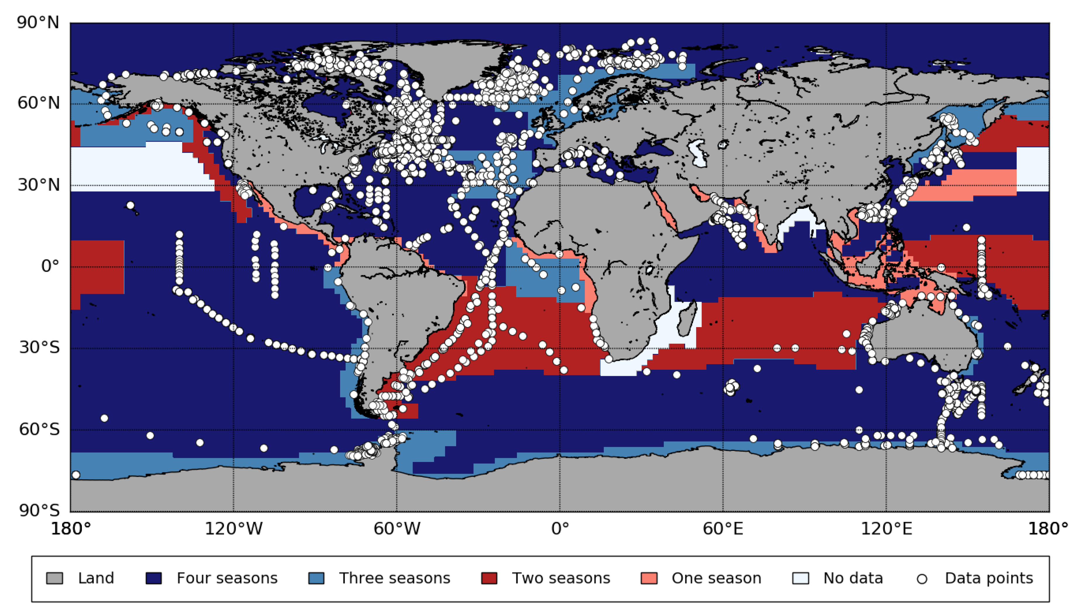
2.3. Photosynthesis versus Irradiance Parameters

Parameters of the photosynthesis versus irradiance (P-I) curve were obtained from a global database [33,56] and additional literature sources [57,58,59,60,61,62,63,64,65,66,67,68,69,70,71,72,73,74,75,76,77,78,79,80,81,82,83,84,85,86,87,88,89,90,91,92,93,94]. A quality check was performed on all data (9765 experiments) following Bouman et al. [33], using lower limits of the initial slope of the P-I curve ${\alpha }^B$ (0.002 mg C mg Chl-a${}^{-1}$ h${}^{-1}$ ($\mathsf{\mu }$mol photons m${}^{-2}$ s${}^{-1}$)${}^{-1}$) and the assimilation number of the P-I curve $P_m^B$ (0.2 mg C mg Chl-a${}^{-1}$ h${}^{-1}$) and an upper limit for the maximum quantum yield of carbon fixation ${\varphi }_m$ (0.15 mol C mol photons${}^{-1}$). The value of ${\varphi }_m$ was calculated as ${\alpha }^B$ / ā${}_B^{\ast }\times 0.0231$ [95] using ${\alpha }^B$ and either simultaneous measurements of the mean specific chlorophyll-a absorption coefficient ā${}_B^{\ast }$ (in m${}^2$ mg Chl-a${}^{-1}$) or an estimate of ā${}_B^{\ast }$ based on Brewin et al. [96], Brewin et al. [97] (see Appendix A). In addition, major outliers in the dataset were identified using the outermost fences of the interquartile range. After quality control, 8676 experiments were used for further analysis. Note that this is a significant improvement over the P-I parameter database that was available at the time of Longhurst et al. [2]; they had access to 1862 P-I observations at that time, mostly from the North Atlantic Ocean.

To estimate regional primary production, P-I data were assigned to biogeographic provinces according to Longhurst [16] (Appendix B). The P-I database covered 53 provinces, representing 96.6% of the world’s oceans (Figure 1). No in situ P-I experiments could be found for the coastal areas of Africa (EAFR) and India (INDE) and two regions in the North Pacific Ocean (NPPF, NPSE). The data were divided into seasons using 3-month intervals; i.e., March–May for spring/autumn, June–August for summer/winter, September–November for autumn/spring and December–February for winter/summer in the Northern/Southern Hemisphere. Mean and standard deviations of ${\alpha }^B$ and $P_m^B$ were calculated for each season and biogeographic province available in the P-I database (

Table 1. Sample size (n), mean and standard deviation (SD) of the initial slope (${\alpha }^B$ in mg C mg Chl-a${}^{-1}$ h${}^{-1}$ ($\mathsf{\mu }$mol photons m${}^{-2}$ s${}^{-1}$)${}^{-1}$) and the assimilation number ($P_m^B$ in mg C mg Chl-a${}^{-1}$ h${}^{-1}$) of the photosynthesis versus irradiance (P-I) curve for each biogeographic province and season. Values in blue are obtained from statistical comparisons between seasons and biogeographic provinces, while other values are directly obtained from the P-I database. Biogeographic provinces are listed in Appendix B.

		Spring						Summer						Autumn						Winter
BIOME		${\mathit{\alpha }}^{\mathit{B}}$			${\mathit{P}}_{\mathit{m}}^{\mathit{B}}$			${\mathit{\alpha }}^{\mathit{B}}$			${\mathit{P}}_{\mathit{m}}^{\mathit{B}}$			${\mathit{\alpha }}^{\mathit{B}}$			${\mathit{P}}_{\mathit{m}}^{\mathit{B}}$			${\mathit{\alpha }}^{\mathit{B}}$			${\mathit{P}}_{\mathit{m}}^{\mathit{B}}$
/BASIN	PROV	n	Mean	SD	n	Mean	SD	n	Mean	SD	n	Mean	SD	n	Mean	SD	n	Mean	SD	n	Mean	SD	n	Mean	SD
Coastal
Atlantic	NECS	18	0.020	0.005	18	3.25	0.64	12	0.022	0.007	15	2.83	1.62	30	0.021	0.006	1	2.22		30	0.021	0.006	34	3.04	1.18
	CNRY	1	0.035		1	4.00		33	0.022	0.006	34	3.92	1.56	11	0.026	0.005	34	4.08	1.70	1	0.016		3	3.30	1.13
	GUIN	1	0.012		1	1.50		48	0.017	0.008	50	1.68	1.04	20	0.017	0.006	19	1.68	0.62	48	0.017	0.008	50	1.68	1.04
	GUIA	77	0.024	0.017	34	2.52	1.88	109	0.023	0.016	56	2.71	1.90	2	0.024	0.008	2	2.71	1.35	109	0.023	0.016	6	2.90	1.21
	NWCS	495	0.031	0.020	515	2.49	1.18	259	0.024	0.017	260	3.23	1.47	335	0.044	0.021	332	3.58	1.66	121	0.037	0.018	125	2.85	1.36
	CHSB	41	0.036	0.018	41	3.29	1.46	35	0.016	0.013	36	2.04	1.66	18	0.041	0.018	19	4.80	1.43	59	0.038	0.018	96	3.12	1.82
	BRAZ	9	0.029	0.016	10	2.22	1.82	48	0.017	0.008	15	2.69	1.95	5	0.014	0.005	5	3.63	2.05	48	0.017	0.008	15	2.69	1.95
	FKLD	28	0.017	0.009	31	1.68	1.24	48	0.017	0.008	50	1.68	1.04	20	0.017	0.006	19	1.68	0.62	48	0.017	0.008	50	1.68	1.04
	BENG	2	0.044	0.000	4	4.24	2.52	25	0.027	0.012	26	3.66	1.67	23	0.026	0.011	22	3.56	1.52	25	0.027	0.012	26	3.66	1.67
Indian	EAFR	117	0.027	0.009	101	4.76	1.66	32	0.030	0.009	17	5.36	1.07	285	0.027	0.011	6	3.43	1.27	280	0.027	0.010	203	4.38	1.62
	REDS	46	0.013	0.007	85	3.29	1.36	4	0.022	0.006	4	4.13	2.07	117	0.027	0.009	101	4.76	1.66	32	0.030	0.009	17	5.36	1.07
	ARAB	13	0.034	0.010	98	4.00	1.48	114	0.024	0.011	81	3.72	1.40	117	0.027	0.009	101	4.76	1.66	32	0.033	0.009	17	5.36	1.07
	INDE	65	0.042	0.021	62	3.39	2.13	5	0.034	0.028	7	4.10	1.53	56	0.034	0.018	56	2.97	1.89	6	0.039	0.015	6	2.50	1.01
	INDW	9	0.033	0.027	6	3.43	1.27	114	0.024	0.011	64	3.94	1.70	117	0.027	0.009	35	3.65	1.48	32	0.030	0.009	29	4.29	1.91
	AUSW	56	0.034	0.018	56	2.97	1.89	6	0.039	0.015	6	2.50	1.01	56	0.047	0.019	56	3.38	2.21	19	0.028	0.017	3	4.05	0.80
Pacific	ALSK	7	0.029	0.012	8	3.91	0.89	61	0.026	0.020	35	4.67	1.90	23	0.023	0.011	43	4.53	1.77	51	0.025	0.010	43	4.53	1.77
	CCAL	42	0.038	0.023	53	3.80	1.76	9	0.012	0.007	26	4.17	1.91	11	0.008	0.001	28	3.21	1.47	2	0.016	0.006	20	1.70	1.08
	CAMR	1	0.026		2	1.50	0.20	31	0.020	0.009	26	4.17	1.91	18	0.026	0.014	28	3.21	1.47	2	0.016	0.006	28	3.48	2.22
	CHIL	8	0.032	0.011	7	2.50	0.93	79	0.031	0.012	78	2.35	1.36	33	0.029	0.010	89	2.35	1.35	4	0.016	0.016	4	2.10	2.12
	CHIN	25	0.026	0.007	17	5.48	1.72	31	0.020	0.009	22	3.59	1.99	18	0.026	0.014	10	4.48	3.23	2	0.016	0.006	2	4.55	1.34
	SUND	26	0.025	0.010	20	4.10	2.30	12	0.041	0.018	16	3.43	2.13	67	0.031	0.012	68	2.85	1.51	11	0.029	0.014	12	2.55	2.13
	AUSE	19	0.050	0.020	320	4.41	1.53	4	0.050	0.018	4	4.65	3.15	31	0.047	0.019	15	2.53	2.13	8	0.042	0.018	11	1.75	0.94
	NEWZ	8	0.045	0.013	9	4.48	1.46	23	0.021	0.011	22	4.63	1.51	9	0.036	0.009	8	3.70	1.42	2	0.044	0.003	2	3.30	0.28
Polar
Antarctic	ANTA	1	0.007		2	1.01	0.92	41	0.018	0.009	75	1.27	0.50	12	0.021	0.005	9	1.58	0.72	54	0.019	0.008	11	1.48	0.74
	APLR	52	0.035	0.009	67	1.66	0.92	268	0.029	0.014	340	1.89	1.26	140	0.026	0.009	162	1.86	0.90	54	0.019	0.008	569	1.86	1.13
Atlantic	BPLR	141	0.031	0.016	154	2.03	0.83	542	0.030	0.017	572	1.67	0.99	189	0.024	0.013	192	1.65	0.84	21	0.031	0.019	21	1.85	0.78
	ARCT	278	0.039	0.017	329	2.38	1.07	298	0.036	0.016	313	2.24	0.99	39	0.032	0.018	59	2.18	0.78	27	0.028	0.013	27	2.38	0.85
	SARC	116	0.044	0.017	126	2.74	1.09	89	0.041	0.014	92	2.59	1.27	206	0.043	0.016	2	1.40	0.46	206	0.043	0.016	220	2.66	1.17
Pacific	BERS	7	0.029	0.012	8	3.26	1.81	21	0.024	0.007	22	2.85	1.18	23	0.023	0.011	25	2.41	1.39	51	0.025	0.010	55	2.71	1.38
Trades
Atlantic	NATR	15	0.025	0.015	14	3.60	1.76	165	0.035	0.021	165	2.85	1.84	27	0.027	0.011	26	2.52	2.40	6	0.032	0.018	7	5.23	1.60
	WTRA	16	0.013	0.007	16	3.06	2.18	109	0.023	0.016	6	2.90	1.21	32	0.025	0.019	34	2.52	21.88	109	0.023	0.016	56	2.71	1.90
	ETRA	4	0.037	0.026	4	2.90	3.23	62	0.026	0.016	61	3.01	1.79	6	0.024	0.014	6	2.97	1.06	52	0.025	0.016	51	3.02	1.76
	SATL	77	0.024	0.017	77	1.99	1.37	109	0.023	0.016	109	1.87	1.35	32	0.020	0.014	32	1.59	1.28	109	0.023	0.016	109	1.87	1.35
	CARB	22	0.010	0.005	21	3.20	1.99	16	0.023	0.010	2	6.25	0.92	25	0.028	0.012	16	5.73	1.76	28	0.022	0.009	28	3.48	2.22
Indian	MONS	5	0.028	0.005	64	3.94	1.70	9	0.024	0.007	64	3.94	1.70	40	0.022	0.007	35	3.65	1.48	35	0.027	0.006	29	4.29	1.91
	ISSG	10	0.007	0.003	10	1.94	1.61	14	0.007	0.003	6	2.50	1.01	4	0.009	0.002	26	2.86	1.31	14	0.007	0.003	3	4.05	0.80
Pacific	NPTG	3	0.013	0.008	9	4.97	0.66	8	0.015	0.003	6	4.39	2.12	10	0.017	0.006	18	4.79	1.70	7	0.016	0.004	26	4.88	0.74
	PNEC	2	0.031	0.011	9	3.46	1.49	12	0.017	0.006	15	3.94	1.85	11	0.017	0.004	27	3.54	1.74	27	0.018	0.005	3	1.75	0.77
	PEQD	11	0.017	0.004	18	4.85	1.58	27	0.018	0.005	6	3.79	1.04	27	0.018	0.005	8	4.76	0.97	16	0.019	0.005	17	4.39	1.33
	WARM	163	0.030	0.015	160	2.23	1.31	220	0.031	0.016	221	2.16	1.28	220	0.031	0.016	221	2.16	1.28	57	0.033	0.020	61	1.97	1.19
	ARCH	67	0.031	0.012	68	2.85	1.51	11	0.029	0.014	12	2.55	2.13	26	0.025	0.010	20	4.10	2.30	19	0.028	0.017	22	2.81	1.92
Westerlies
Antarctic	SSTC	18	0.021	0.016	47	4.12	2.01	45	0.034	0.011	83	2.25	1.56	33	0.029	0.010	53	4.42	1.39	4	0.016	0.016	5	5.30	1.57
	SANT	3	0.026	0.002	28	1.85	0.42	41	0.023	0.006	136	1.58	0.53	10	0.027	0.003	18	1.99	0.54	55	0.023	0.006	242	1.62	0.54
Atlantic	NADR	47	0.032	0.014	42	3.32	1.25	4	0.051	0.023	4	3.03	0.73	49	0.025	0.014	52	2.14	1.20	7	0.036	0.007	7	2.83	0.45
	GFST	50	0.034	0.012	47	4.39	1.60	14	0.013	0.006	13	2.40	1.99	24	0.040	0.016	28	3.08	1.67	7	0.054	0.020	7	4.32	2.06
	NASW	137	0.031	0.018	96	3.84	2.53	113	0.029	0.021	92	2.13	1.85	65	0.036	0.024	57	4.09	2.23	33	0.041	0.019	30	4.66	1.35
	MEDI	46	0.013	0.007	85	3.29	1.36	26	0.005	0.003	36	2.65	1.86	77	0.032	0.021	113	2.57	1.66	55	0.040	0.019	105	2.64	1.35
	NASE	25	0.029	0.018	27	3.95	1.78	17	0.030	0.009	17	2.72	1.67	44	0.025	0.014	60	2.86	2.01	86	0.031	0.018	7	5.23	1.60
Pacific	PSAE	18	0.035	0.014	18	2.48	0.74	42	0.032	0.013	46	2.54	0.81	8	0.025	0.012	9	2.35	1.06	68	0.032	0.013	73	2.50	0.82
	PSAW	33	0.039	0.011	31	3.32	0.93	8	0.036	0.018	8	3.51	1.55	41	0.038	0.013	39	3.36	1.06	41	0.038	0.013	39	3.36	1.06
	KURO	83	0.020	0.009	81	3.62	1.64	61	0.017	0.007	60	2.88	1.41	82	0.020	0.007	86	3.62	1.70	10	0.021	0.009	9	4.63	0.52
	NPPF	134	0.027	0.013	144	3.28	1.46	111	0.024	0.013	114	2.79	1.23	96	0.020	0.008	100	3.48	1.65	10	0.021	0.009	9	4.63	0.52
	NPSE	134	0.027	0.013	144	3.28	1.46	111	0.024	0.013	114	2.79	1.23	96	0.020	0.008	100	3.48	1.65	10	0.021	0.009	9	4.63	0.52
	NPSW	83	0.020	0.009	81	3.62	1.64	61	0.017	0.007	60	2.88	1.41	6	0.015	0.005	5	3.22	0.59	10	0.021	0.009	9	4.63	0.52
	OCAL	10	0.007	0.002	10	1.87	0.59	12	0.017	0.006	46	2.54	0.81	1	0.006		9	2.35	1.06	10	0.021	0.009	73	2.50	0.82
	TASM	8	0.053	0.017	12	5.10	1.51	19	0.053	0.013	25	4.68	2.04	3	0.029	0.001	19	5.99	1.54	12	0.053	0.012	13	4.52	1.22
	SPSG	240	0.021	0.015	246	1.79	1.33	27	0.022	0.011	29	1.35	0.79	3	0.029	0.001	281	1.77	1.30	4	0.025	0.004	6	3.16	1.37

). Temporal and spatial data gaps in ${\alpha }^B$ and $P_m^B$ were filled by statistical analysis of the relationships between seasons within each biogeographic province and the relationships between adjacent biogeographic provinces (Figure 2). To this end, values of ${\alpha }^B$ and $P_m^B$ were log-transformed and significance ($p<0.05$) was tested using ANOVA analysis followed by Tukey-Kramer post-hoc testing for unequal sample sizes (Past 3, Hammer et al. 2001). Results were used to assign mean and standard deviations of ${\alpha }^B$ and $P_m^B$ for missing seasons and/or biogeographic provinces (Table 1) respecting boundaries of the ocean basins and biomes [16]. Linear- and log-scaled mean values of ${\alpha }^B$ and $P_m^B$ were highly similar (r${}^2$ = 0.989, p < 0.001, with the majority of data normally distributed on regional and seasonal scales), and calculations of primary production were performed with the linear-scaled mean and standard deviation of each P-I parameter (Table 1) to support interpretation of (linear) trends in the sensitivity analyses (see below).

2.4. Analyses of Primary Production

The sensitivity of primary production to changes in photosynthetic parameters was estimated using three separate model runs for the period between 1998 and 2018, with three different P-I parameters assignments as follows: (a) with the mean of the P-I parameters for each of the provinces and seasons (the main run); (b) with the mean minus one standard deviation of the two P-I parameters (–1 SD); and (c) with the mean plus one standard deviation of the two P-I parameters (+1 SD) (Table 1). All other input variables (i.e., light, chlorophyll-a and chlorophyll-a profile parameters) were kept the same for each of these model runs. To assess the magnitude of change in primary production with change in individual P-I parameters, an additional sensitivity analysis was performed for a sample year (arbitrarily chosen to be 2003) in which either ${\alpha }^B$ or $P_m^B$ was adjusted by ±1 standard deviation, while the other parameter was maintained at its mean value. In the full model computations in which ${\alpha }^B$ and $P_m^B$ were adjusted simultaneously, the relationship between ${\alpha }^B$ and $P_m^B$, given by the light adaptation parameter ($I_k$ in $\mathsf{\mu }$mol photons m${}^{-2}$ s${}^{-1}$), remained largely unchanged. In the additional sensitivity analysis $I_k$ was allowed to vary and increased for −1 SD ${\alpha }^B$ and +1 SD $P_m^B$ and decreased for +1 SD ${\alpha }^B$ and −1 SD $P_m^B$. For all model computations, both annual and seasonal primary production rates were estimated on global and regional scales. Regions were selected based on Longhurst’s definitions of ocean basins (Antarctic, Atlantic, Indian and Pacific) and biomes (Coastal, Polar, Trades and Westerlies) [16].

Statistical analyses were used to assess relationships between P-I parameters and other (environmental) variables available in the P-I database (latitude, depth, chlorophyll-a, PAR, temperature and nutrients; correlation and regression analysis), relationships between primary production estimates and input variables (chlorophyll-a, PAR and P-I parameters; correlation and regression analysis) and changes in primary production trends on various spatial and temporal scales (correlation analysis). To estimate the rate and direction of change in annual primary production between 1998 and 2018 for each grid point, monthly means were corrected for seasonality by subtracting monthly climatologies. The rate of change over time and its significance were calculated using linear regression and Student’s t tests following Santer et al. [98]. Using the slope and intercept from the regression analysis, the percentage change per year in primary production (PP) was calculated as $100·((12·slope)/(intercept+P{P}_{climatology}))$. Before all statistical procedures, data were tested for normality and homogeneity of variances and transformed for further statistical analysis when necessary. Differences were considered significant when p < 0.05.

The impacts of different climate indices on global and regional primary production were characterised based on annual mean anomalies that were corrected for seasonality following Racault et al. [19]. Student’s t tests were used to assess the statistical significance of the relationships considering autocorrelations of the time series following Santer et al. [98]. Climate indices were obtained from the National Oceanic and Atmospheric Administration (NOAA) (www.esrl.noaa.gov/psd/data/climateindices/), Kao and Yu [99] (www.ess.uci.edu/~yu/2OSC/) and Di Lorenzo et al. [17] (www.o3d.org/npgo/).

3. Results

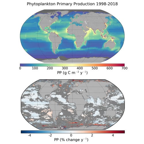
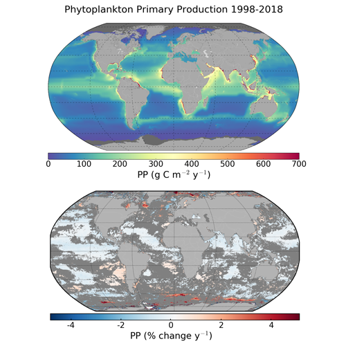
3.1. Global and Regional Annual Primary Production

Global annual primary production computed using mean photosynthesis versus irradiance (P-I) parameters (for each biogeographic province and for each season) varied from 48.7 to 52.5 Gt C y⁻¹ in the period 1998–2018 (

Table 2. Climatological mean and standard deviation (n = 21) of annual primary production (in Gt C y${}^{-1}$) between 1998 and 2018 for each ocean basin and biome as defined by Longhurst (2007). Range in annual primary production between 1998 and 2018 is given in parentheses. Results are given for primary production estimates based on mean, −1 standard deviation and +1 standard deviation photosynthesis versus irradiance (P-I) parameters. Surface areas (in km${}^2$) for each ocean basin and biome are also provided.

Mean P-I
		Coastal	Polar	Trades	Westerlies	Total
		47 × 106	57 × 106	141 × 106	131 × 106	376 × 106
Antarctic	79 × 106		1.06 ± 0.09 (0.88−1.21)		4.83 ± 0.14 (4.66–5.14)	5.88 ± 0.19 (5.58–6.20)
Atlantic	94 × 106	3.13 ± 0.16 (2.89–3.33)	1.54 ± 0.09 (1.39–1.76)	6.52 ± 0.14 (6.24–6.73)	3.12 ± 0.05 (3.04–3.24)	14.3 ± 0.38 (13.7–14.9)
Indian	48 × 106	3.82 ± 0.18 (3.55–4.10)		4.42 ± 0.12 (4.17–4.62)		8.24 ± 0.30 (7.72–8.70)
Pacific	155 × 106	4.76 ± 0.22 (4.34–5.03)	0.91 ± 0.06 (0.80–1.02)	9.21 ± 0.31 (8.57–9.62)	7.39 ± 0.16 (7.09–7.60)	22.3 ± 0.63 (21.2–23.1)
Total	376 × 106	11.7 ± 0.53 (10.9–12.4)	3.51 ± 0.20 (3.12–3.85)	20.2 ± 0.50 (19.1–20.7)	15.3 ± 0.30 (15.0–15.9)	50.7 ± 1.38 (48.7–52.5)
Mean P-I –1 Standard Deviation
		Coastal	Polar	Trades	Westerlies	Total
		47 × 106	57 × 106	141 × 106	131 × 106	376 × 106
Antarctic	79 × 106		0.56 ± 0.04 (0.48–0.64)		2.82 ± 0.09 (2.72–3.02)	3.39 ± 0.11 (3.22–3.59)
Atlantic	94 × 106	1.64 ± 0.08 (1.51–1.76)	0.81 ± 0.05 (0.73–0.90)	2.52 ± 0.06 (2.39–2.61)	1.51 ± 0.03 (1.47–1.56)	6.48 ± 0.19 (6.16–6.75)
Indian	48 × 106	2.27 ± 0.10 (2.11–2.42)		2.70 ± 0.08 (2.54–2.82)		4.96 ± 0.17 (4.65–5.24)
Pacific	155 × 106	2.35 ± 0.11 (2.12–2.49)	0.52 ± 0.03 (0.45–0.58)	5.13 ± 0.18 (4.75–5.34)	4.00 ± 0.09 (3.85–4.12)	12.0 ± 0.34 (11.4–12.5)
Total	376 × 106	6.26 ± 0.28 (5.79–6.64)	1.89 ± 0.10 (1.70–2.06)	10.3 ± 0.27 (9.75–10.6)	8.34 ± 0.17 (8.13–8.66)	26.8 ± 0.74 (25.7–27.8)
Mean P-I +1 Standard Deviation
		Coastal	Polar	Trades	Westerlies	Total
		47 × 106	57 × 106	141 × 106	131 × 106	376 × 106
Antarctic	79 × 106		1.49 ± 0.14 (1.24–1.71)		6.71 ± 0.19 (6.48–7.14)	8.20 ± 0.26 (7.78–8.63)
Atlantic	94 × 106	4.57 ± 0.23 (4.21–4.86)	2.27 ± 0.14 (2.05–2.61)	10.4 ± 0.22 (9.95–10.7)	4.70 ± 0.08 (4.58–4.87)	21.9 ± 0.58 (20.9–22.8)
Indian	48 × 106	5.34 ± 0.26 (4.96–5.72)		6.07 ± 0.17 (5.71–6.34)		11.4 ± 0.42 (10.7–12.0)
Pacific	155 × 106	7.08 ± 0.32 (6.47–7.49)	1.30 ± 0.08 (1.13–1.46)	13.2 ± 0.44 (12.3–13.8)	10.6 ± 0.23 (10.2–10.9)	32.1 ± 0.92 (30.6–33.4)
Total	376 × 106	17.0 ± 0.77 (15.8–18.0)	5.07 ± 0.30 (4.48–5.56)	29.6 ± 0.73 (28.1–30.4)	22.0 ± 0.43 (21.5–22.8)	73.7 ± 2.00 (70.8–76.2)

; Figure 3 and Figure 4A). Summer (14.6–16.0 Gt C) was the most productive season in each of the years, followed by spring (13.5–14.7 Gt C), autumn (11.0–11.9 Gt C per season) and winter (9.4–10.2 Gt C per season) (Figure 4B). On regional scales, annual primary production was highest in the Pacific Ocean (43.2–44.5%), followed by the Atlantic (27.8–28.8%), Indian (15.7–16.7%) and Antarctic oceans (11.3–12.0%) (Table 2; Figure 3). In addition, the highest annual primary production rates were found at low latitudes in the Trades biome (39.2–40.7%), followed by the Westerlies (29.7–31.1%), Coastal (22.2–23.7%) and Polar biomes (6.3–7.3%) (Table 2; Figure 3). These regional differences in annual primary production were related to the surface areas of the specific ocean basins and biomes (r² = 0.674, p < 0.01), with the coastal regions being relatively more and polar regions relatively less productive than the other regions when computed as a rate per unit area (Table 2; Figure 3A).

3.2. Trends in Primary Production

Linear trends in annual primary production between 1998 and 2018 varied considerably on regional scales (Figure 3B). At low and mid latitudes, trends in primary production were generally weak and negative (up to −3.0%), although large areas of positive trends were also observed in the South Atlantic Ocean and the South Pacific Ocean. In polar and coastal (upwelling) regions, stronger, positive trends in primary production were observed (up to +4.5%). Although significant linear trends were observed at individual pixels, the observed inter-annual changes in primary production on global and regional scales did not follow a linear pattern.

Inter-annual trends in global primary production showed an increase in rates between 1998 and 2003; relatively stable rates between 2003 and 2011; and a subsequent decrease in rates until 2015, after which rates showed a minor increase (Figure 4A). Annual primary production in the Atlantic and Pacific oceans showed similar inter-annual trends to global primary production (r${}^2$ = 0.856, 0.913, p < 0.001) (Figure 4C). Trends in annual primary production in the other ocean basins varied from the global trend, with relatively lower production between 2003 and 2011 in the Antarctic Ocean (r${}^2$ = 0.712, p < 0.001) and a relatively early decrease in production in the Indian Ocean (r${}^2$ = 0.767, p < 0.001) (Figure 4C). Annual primary production in the Coastal, Trades and Westerlies biomes showed inter-annual trends comparable with that in global primary production (r${}^2$ = 0.794–0.922, p < 0.001), with relatively higher rates observed between 1998 and 2000 in the Trades biome and a relatively slow increase in production between 1998 and 2011 in the Westerlies biome (Figure 4E). In the Polar biome, production decreased relatively early between 2004 and 2011 and was relatively high after 2015 compared with the trends in global annual primary production (r${}^2$ = 0.583, p < 0.001).

Trends in seasonal global primary production were highest in late spring to mid-summer, with the lowest rates observed in December for the Northern Hemisphere and in June for the Southern Hemisphere (Figure 4B). Most regions showed similar seasonal trends in primary production, with the peak occurring either earlier (Pacific Ocean and Westerlies and Coastal biomes) or later (Antarctic and Atlantic oceans and Polar biome) in summer (r${}^2$ = 0.790–0.958, p < 0.001) (Figure 4D,F). Monthly primary production in the Trades biome was more variable from spring to autumn compared with the global trend (r${}^2$ = 0.758, p < 0.001) (Figure 4D). Trends in seasonal primary production in the Indian Ocean deviated most from the global trend, with two peaks in monthly primary production observed in spring and autumn and the lowest rates observed in summer (Figure 4F).

Inter-annual and seasonal trends in global primary production were closely related to chlorophyll-a biomass (Spearman’s rank correlation coefficient $r_s$ = 0.661–0.939, p < 0.01) (Figure 3C). In the Pacific Ocean and Westerlies biome, annual primary production was also related to Photosynthetic Active Radiation (PAR) ($r_s$ = 0.438–0.436, p < 0.05) (Figure 3E). The variations in global primary production were associated with trends in the El Niño-Southern Oscillation (ENSO) (Multi-variate ENSO Index (MEI), r = −0.309; ENSO Eastern Pacific (EP) index, r = −0.469) and the Atlantic Multidecadal Oscillation (AMO) (r = 0.419). The initial increase in global annual primary production between 1998 and 2003 was related to ENSO (EP index, r = −0.956), AMO (r = 0.971) and the Indian Ocean Dipole (IOD) (r = 0.563), while the decrease in global annual primary production after 2011 was related to ENSO (MEI, r = −0.664; ENSO Central Pacific (CP) index, r = −0.883) and the Pacific Decadal Oscillation (PDO) (r = −0.832).

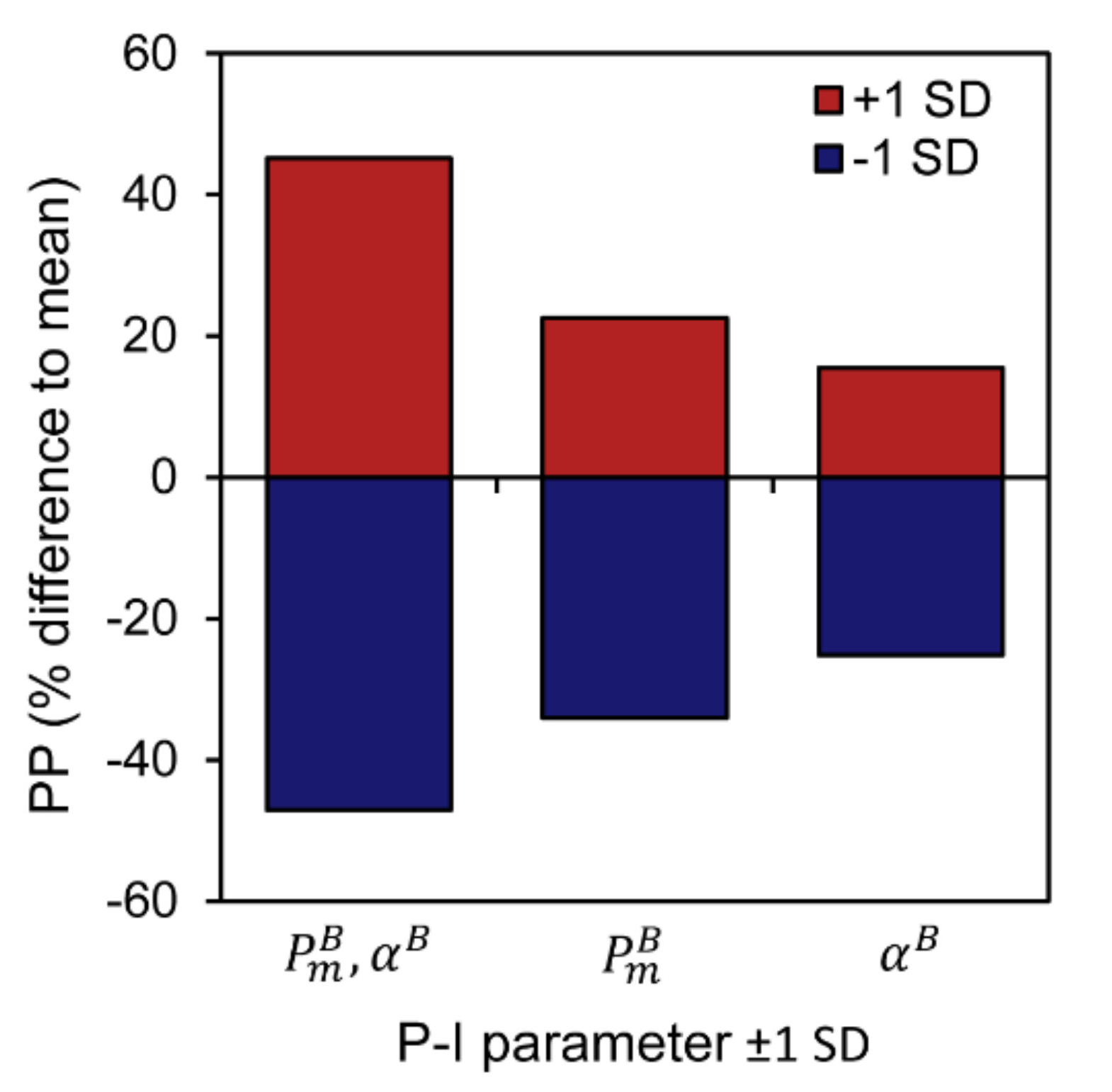
3.3. Sensitivity of Primary Primary Production to Changes in Photosynthetic Parameters

Global annual primary production varied from 25.7 to 27.8 Gt C y${}^{-1}$ between 1998 and 2018 when both P-I parameters were reduced simultaneously by one standard deviation (−1 SD), whereas the values ranged from 70.8 to 76.2 Gt C y${}^{-1}$ when the P-I parameters were increased by one standard deviation (+1 SD) (−46.4% and +44.8% compared with the results using the mean P-I estimates) (Table 2; Figure 3D,F and Figure 5). The magnitude of the decrease in primary production when the P-I parameters were adjusted by −1 standard deviation was always greater than the increase in production when the P-I parameters were adjusted by +1 standard deviation (Figure 5). The sensitivity of primary production to changes in P-I parameters was highest in the Atlantic Ocean, followed by the Pacific, Antarctic and Indian oceans (Figure 3D,F and Figure 5; Table 2). The sensitivity was highest in the Trades biome and lowest in the Westerlies biome (Figure 3D,F and Figure 5; Table 2). Trends in global and regional annual primary production for the sensitivity analyses (data not shown) were similar to those observed for the main model run with mean P-I parameters (Table 2; Figure 3B and Figure 4) (r${}^2$ = 0.983–0.999, p < 0.001).

On a seasonal basis, global primary production changed between −50.1 to −43.9% and +42.2 to +48.5% when the photosynthetic parameters were adjusted by −1 and +1 standard deviation, respectively (Figure 5). The highest deviation from the mean P-I-based primary production estimates was observed during summer in the Atlantic Ocean and during spring in the Trades biome, whereas the lowest deviation was observed during autumn in the Antarctic Ocean and during winter in the Westerlies biome. Trends in seasonal primary production were similar to those observed for the mean photosynthetic parameters estimates (Figure 4) when the photosynthetic parameters were adjusted by +1 standard deviation (data not shown). When the photosynthetic parameters were adjusted by −1 standard deviation, seasonal trends changed in the Indian Ocean and the Coastal and Trades biomes. Primary production in these regions became relatively lower in spring and summer compared with other seasons (data not shown). No changes in seasonal primary production trends were observed in the Antarctic, Atlantic and Pacific oceans and the Polar and Westerlies biomes when photosynthetic parameters were adjusted by −1 standard deviation.

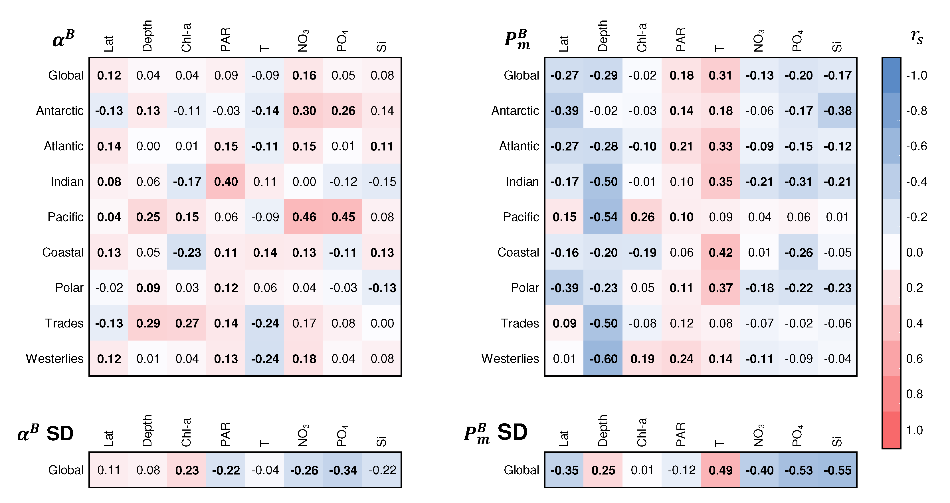
3.4. Relationship between Photosynthetic Parameters and Primary Production

It was expected that the changes in the magnitude of global and regional primary production were driven by variations in photosynthetic parameters, as all other input variables remained unchanged between the different model computations. When the relative change in primary production was compared with that of the P-I parameters for −1 SD and +1 SD estimates, variations were shown to be closely coupled (the light adaptation parameter $I_k$ was unchanged) (Figure 6). Both the initial slope of the P-I curve (${\alpha }^B$) (r${}^2$ = 0.536 for −1 SD and r${}^2$ = 0.571 for +1 SD estimates) and the assimilation number ($P_m^B$) (r${}^2$ = 0.711 for −1 SD and r${}^2$ = 0.670 for +1 SD estimates) showed positive linear relationships with primary production for each season and biogeographical province. The weaker sensitivity of daily water-column primary production to change in ${\alpha }^B$, relative to that of $P_m^B$, could be explained by the importance of ${\alpha }^B$ under light-limited conditions, as opposed to $P_m^B$, whose effect is dominant in light-saturating conditions. It is important to note that the ratio of $P_m^B$ to ${\alpha }^B$ (i.e., $I_k$) remained unchanged between these different estimates of primary production. Independent variations in ${\alpha }^B$ and $P_m^B$ that modify $I_k$ could lead to higher sensitivity of primary production to the change [100,101,102,103]. The sensitivity analysis in which ${\alpha }^B$ and $P_m^B$ were independently adjusted by ±1 standard deviation (variable $I_k$) showed that changes in $P_m^B$ caused greater variation in global annual primary production than changes in ${\alpha }^B$ (Figure 7). Significant relationships between P-I parameters and primary production were also observed when ${\alpha }^B$ and $P_m^B$ were varied independently (−1 SD ${\alpha }^B$: $y=0.617x$, r${}^2$ = 0.862; +1 SD ${\alpha }^B$: $y=0.369x$, r${}^2$ = 0.534; −1 SD $P_m^B$: $y=0.704x$, r${}^2$ = 0.893; +1 SD $P_m^B$: $y=0.444x$, r${}^2$ = 0.723). When $I_k$ increased (−1 SD ${\alpha }^B$ and +1 SD $P_m^B$), primary production became more sensitive to changes in $P_m^B$ compared with those in ${\alpha }^B$ (see slope of relationships above).

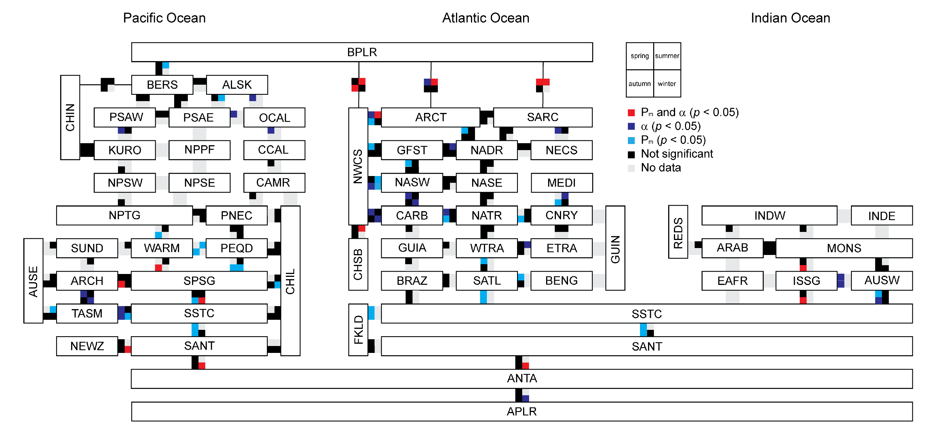
3.5. Variation in Photosynthetic Parameters

In the global P-I parameter database ${\alpha }^B$ ranged between 0.002–0.085 mg C mg Chl-a${}^{-1}$ h${}^{-1}$ ($\mathsf{\mu }$mol photons m${}^{-2}$ s${}^{-1}$)${}^{-1}$ and $P_m^B$ between 0.20–8.00 mg C mg Chl-a${}^{-1}$ h${}^{-1}$. Mean values for each biogeographic province ranged between 0.005 and 0.054 mg C mg Chl-a${}^{-1}$ h${}^{-1}$ ($\mathsf{\mu }$mol photons m${}^{-2}$ s${}^{-1}$)${}^{-1}$ for ${\alpha }^B$ and between 1.01 and 6.25 mg C mg Chl-a${}^{-1}$ h${}^{-1}$ for $P_m^B$ (Table 1). Lowest mean values of ${\alpha }^B$ and $P_m^B$ were observed in the Mediterranean (MEDI, summer) and Antarctic (ANTA, spring) provinces, whereas the highest values were observed in the Gulf Stream (GFST, winter) and Caribbean (CARB, summer) provinces, respectively (Table 1). Standard deviations varied between 0.2 and 99.1% (average of 43.8%) for ${\alpha }^B$ and between 8.6 and 111.6% (average of 47.1%) for $P_m^B$ (Table 1). Similar to observations reported in Bouman et al. [33], spatial and temporal variations in photosynthetic parameters could be related to local environmental conditions. Relationships between ${\alpha }^B$ and environmental conditions were variable between ocean basins and biomes resulting in relative weak relationships on a global scale (Figure 8). The initial slope ${\alpha }^B$ increased with daily PAR in the Atlantic and Indian Oceans and with nitrate concentrations in the Antarctic, Atlantic and Pacific Oceans (Figure 8). Positive relationships between ${\alpha }^B$ and chlorophyll-a were observed at mid latitudes (Trades biome), but a negative relationship was observed in the Coastal biome. The standard deviation of ${\alpha }^B$ increased at lower levels of PAR, at lower nitrate and silicate concentrations and at higher chlorophyll-a concentrations, but no other significant relationships with environmental parameters were observed (Figure 8). The assimilation number $P_m^B$ showed overall stronger relationships with environmental conditions compared with ${\alpha }^B$ (Figure 8). Notably, $P_m^B$ increased with temperature and PAR, possibly coinciding with latitudinal differences (Figure 8). The Pacific Ocean deviated from these results with an opposite trend observed between $P_m^B$ and temperature at higher latitudes (data not shown). A negative relationship was observed between $P_m^B$ and depth in all ocean basins and biomes, consistent with the known decline in $P_m^B$ with decreasing temperature and light. $P_m^B$ was generally lower at low phosphate concentrations, with the strongest relationships observed in the Antarctic, Atlantic and Indian Oceans at higher latitudes in the Polar and Coastal biomes. Variation in $P_m^B$ as expressed by the standard deviation increased at higher temperatures and lower latitudes (Figure 8). The standard deviation of $P_m^B$ also showed a positive relationship with depth and negative relationships with nutrient conditions.

4. Discussion

In the present study, a global database of photosynthesis versus irradiance (P-I) parameters, together with a 20-year time series of remote-sensing-based chlorophyll-a concentrations, was used to study the magnitude and variability in marine primary production on a global scale. The estimate for global annual primary production of 48.7–52.5 Gt C y${}^{-1}$ between 1998 and 2018 in this study was within the range reported before (32.0–70.7 Gt C y${}^{-1}$) [5,104] and close to earlier reported values for depth- and wavelength-resolved primary production models (45–56 Gt C y${}^{-1}$) [2,4,5,7,22]. According to the model used in this study, primary production depends on phytoplankton biomass (in chlorophyll units), Photosynthetic Active Radiation (PAR, 400–700 nm; total value and its spectral and angular distribution) and on the assigned values of the photosynthetic and chlorophyll-a profile parameters. Although the model does not explicitly include the effects of environmental variables such as temperature and nutrients, or mixed-layer dynamics, these were implicitly accounted for through the photosynthetic and chlorophyll-a profile parameters, which were assigned by season and biogeographical province [2,16]. Based on an inter-comparison of various primary production models, it has been reported that primary production generally increases at higher chlorophyll-a concentrations, higher PAR and shallower mixed-layer depths, whereas variability in temperature could either increase or decrease primary production [4]. In the present study, trends in global and regional annual primary production were best explained by variations in chlorophyll-a concentration, which in turn may vary with seasonal, inter-annual and multi-decadal variations in physico-chemical conditions of the water column [17,18,19]. This study confirmed that global annual primary production varied with the ENSO and AMO [17,18,19,26], but not all variation in global annual primary production could be explained by large-scale ocean-atmospheric oscillations. The previously reported negative (linear) trend in global annual primary production [25,27,28] was not observed in the present study. Instead, a more dynamic pattern of inter-annual trends in primary production was revealed at global and regional scales (also see [26,29]).

The assignment of photosynthetic parameters remains one of the major challenges in the assessment of global annual primary production using numerical models based on remote-sensing observations [31,32,33,34]. In this study, we have tackled this problem by assembling a database of around ten thousand observations that covered the majority of the biogeographical provinces of Longhurst [16]. The sensitivity of primary production to variations in the photosynthetic parameters was further studied by investigating the effect on primary production of changing P-I parameters from their mean values. P-I parameters may vary 2–10-fold among different biogeographical provinces (this study; [33,86,105]). This variation may reflect natural variability but might also be affected to some extent by small differences in measurement protocols from author to author [33,86]. In the database used here, we tried to minimise the latter source of variability, for example by correcting values of the initial slope of the P-I curve (${\alpha }^B$) for the spectral quality of the light source used in the P-I experiment (also see [33]). A sensitivity analysis in which P-I parameters were adjusted by ±1 standard deviation revealed that the variation in photosynthetic rates may lead to a decrease or an increase in the magnitude of global annual primary production by 45–47%. Global annual primary production remained close to the range of earlier observations (32.0–70.7 Gt C y${}^{-1}$) [2,4,5,22] when both P-I parameters were adjusted by +1 standard deviation (+1 SD) (70.8–76.2 Gt C y${}^{-1}$), but adjustments by −1 standard deviation (−1 SD) resulted in considerably lower global annual primary production rates (25.7–27.8 Gt C y${}^{-1}$). Seasonal trends in global primary production were little affected, as the magnitude of change in P-I parameters was similar among seasons. The sensitivity analysis illustrated the importance of the parameters that describe the relationship between phytoplankton biomass and PAR in the calculations of primary production, but adjusting the P-I parameters by ±1 standard deviation would represent the lower and upper limits of change in the photosynthetic response of phytoplankton cells. It would therefore be important to better understand the variability in P-I parameters and subsequent estimates of primary production under natural variations in environmental conditions and under global climate change.

Over the past three decades, considerable efforts have been made to establish a global database of P-I parameters ([2,31,33,86]; this study) and to decipher their empirical relationships with physico-chemical and optical properties to enable prediction of photosynthetic parameters on regional and global scales [38,40,41,105,106,107,108]. The observed relationships between physico-chemical conditions and P-I parameters in the present study confirmed earlier observations that temperature may be a good predictor of the assimilation number ($P_m^B$), especially in coastal regions and temperate oceanic regions where temperature and associated water column stability dictates seasonal changes in the taxonomic and size structure of phytoplankton communities [40,86,109]. We note however, that the correlation coefficient between $P_m^B$ and temperature is nowhere higher than 0.42, indicating that the importance of other factors (such as light and nutrient availability) in determining the variability in the assimilation number cannot be ruled out. The temperature dependence of $P_m^B$ is of particular interest for assigning photosynthetic rates on regional and global scales, as Sea Surface Temperature (SST) can be obtained from remote-sensing observations on similar spatial and temporal scales to chlorophyll-a concentrations. Moreover, SST is a strong predictor of global climate change [24]. However, in regions with different underlying physical forcing that experience a smaller range in temperature, such as the Arabian Sea and open ocean gyres, the relationship between temperature and $P_m^B$ is less obvious (this study; [40,41,105,107,110]). In such regions, chlorophyll-a concentration and the taxonomic and size structure of the phytoplankton community may be better indicators of variability in $P_m^B$ [38,41,86,107,108]. The initial slope of the P-I curve seems to be more difficult to predict based on empirical relationships with physico-chemical conditions (this study, [41,86]), and it has been suggested that the simplest approach to estimate ${\alpha }^B$ would be to relate ${\alpha }^B$ to the assimilation number [33,110,111]. This approach may be supported by the strong dependence of $I_K$ ($P_m^B$/${\alpha }^B$) on latitude and depth, two spatial indicators that can be seen as general proxies of water column conditions [16,33,105].

The relationship between photosynthetic parameters and temperature is of particular interest in understanding the scope of change in primary production under global climate change. Over the past few decades, SST has increased by 0.5 ${}^{ }$C and is projected to increase a further 1.5–4.0 ${}^{ }$C under different CO${}_2$ emission scenarios [24]. The rise in SST and subsequent changes in stratification and nutrient loading into the euphotic zone are expected to affect phytoplankton growth and primary production [23,24]. One estimate of a potential change in annual primary production arising from variations in photosynthetic parameters under global climate change can be arrived at by using SST as the main driver of change in $P_m^B$. Assuming a simplified linear relationship between $P_m^B$ and temperature in the Coastal biome (where temperature dependence of $P_m^B$ was highest; $P_m^B=0.13\ast T+1.82$, $r^2$ = 0.872 for T < 20 ${}^{ }$C), $P_m^B$ might be expected to increase by 8.3% under a rise of SST of +2 ${}^{ }$C. Based on the relationships between $P_m^B$ and primary production estimates presented in this study (Figure 7; assuming $I_k$ is unchanged), annual primary production in the Coastal biome could increase by +0.92 Gt C y${}^{-1}$. Depending on the specific relationship with temperature, variations in P-I parameters and subsequent estimates of global primary production may vary on regional scales (for example, +13.4% in $P_m^B$ in the Polar biome). The actual variation in P-I parameters and primary production under global climate change would be more complex and the interplay between different physico-chemical conditions will have a major effect on the direction of change.

5. Conclusions

It is the first time that highly quality-controlled, multi-sensor, inter-sensor-bias-corrected, ocean-colour observations extending over two decades have been combined with the increased spatial and temporal coverage of in situ observations of the photosynthetic parameters of phytoplankton to compute the magnitude and variability of primary production on a global scale. This has led to a more accurate assessment of global annual primary production and its trends over the past 20 years. Variability in global annual primary production could be related to inter-annual and multi-decadal oscillations, such that the present record of ocean-colour observations is not of sufficient length to detect trends associated with climate change [112]. Here, we report an inter-annual variability (standard deviation) of ±2.7% around a mean of 50.7 Gt C y⁻¹ within the two decades studied. The importance of accurately assigning photosynthetic parameters in global and regional calculations of primary production has been illustrated by a sensitivity analysis. With the recent development of a global database of in situ measurements of P-I parameters [33] and the subsequent enhancement of the database (this study), photosynthetic parameters could be assigned to almost all biogeographical provinces (defined by Longhurst [16]). This has considerably improved the confidence with which regional primary production can be estimated, especially in those regions that were previously known to be different from others, such as the Arabian Sea and the Antarctic Ocean [110]. Yet, the need to improve P-I data coverage in large areas of the global ocean remains (this study, Figure 1; [33,49,86]). In particular, large areas of the Pacific and Indian oceans remain poorly sampled. Methods designed to assign photosynthetic parameters based on their relationships to other variables amenable to remote sensing [106,110] could, in the future, lead to a more dynamic assignment of these parameters. Sea-surface temperature and phytoplankton community-size structure (this study; [33,38,40,41,86,105,107,108]) could be suitable variables for further development of such methods for different ocean basins and biomes.

References

1. Lurin, B.; Rasool, S.; Cramer, W.; Moore, B. Global terrestrial net primary production. Glob. Chang. Newsl. 1994, 19, 6–8. [Google Scholar]
2. Longhurst, A.R.; Sathyendranath, S.; Platt, T.; Caverhill, C. An estimate of global primary production in the ocean from satellite radiometer data. J. Plankton Res. 1995, 17, 1245–1271. [Google Scholar] [CrossRef] [Green Version]
3. Field, C.B. Primary Production of the Biosphere: Integrating Terrestrial and Oceanic Components. Science 1998, 281, 237–240. [Google Scholar] [CrossRef] [PubMed] [Green Version]
4. Carr, M.E.; Friedrichs, M.A.; Schmeltz, M.; Noguchi Aita, M.; Antoine, D.; Arrigo, K.R.; Asanuma, I.; Aumont, O.; Barber, R.; Behrenfeld, M.; et al. A comparison of global estimates of marine primary production from ocean color. Deep-Sea Res. Part II Top. Stud. Oceanogr. 2006, 53, 741–770. [Google Scholar] [CrossRef] [Green Version]
5. Buitenhuis, E.T.; Hashioka, T.; Quéré, C.L. Combined constraints on global ocean primary production using observations and models. Glob. Biogeochem. Cycles 2013, 27, 847–858. [Google Scholar] [CrossRef]
6. Falkowski, P.G.; Barber, R.T.; Smetacek, V. Biogeochemical controls and feedbacks on ocean primary production. Science 1998, 281, 200–206. [Google Scholar] [CrossRef] [Green Version]
7. Antoine, D.; André, J.M.; Morel, A. Oceanic primary production 2. Estimation at global scale from satellite (coastal zone color scanner) chlorophyll. Glob. Biogeochem. Cycles 1996, 10, 57–69. [Google Scholar] [CrossRef]
8. von Schuckmann, K.; Le Traon, P.Y.; Alvarez-Fanjul, E.; Axell, L.; Balmaseda, M.; Breivik, L.A.; Brewin, R.J.; Bricaud, C.; Drevillon, M.; Drillet, Y.; et al. The Copernicus Marine Environment Monitoring Service Ocean State Report. J. Oper. Oceanogr. 2016, 9, s235–s320. [Google Scholar] [CrossRef]
9. Le Quéré, C.; Andrew, R.; Friedlingstein, P.; Sitch, S.; Hauck, J.; Pongratz, J.; Pickers, P.; Ivar Korsbakken, J.; Peters, G.; Canadell, J.; et al. Global Carbon Budget 2018. Earth Syst. Sci. Data 2018, 10, 2141–2194. [Google Scholar] [CrossRef] [Green Version]
10. Sathyendranath, S.; Brewin, R.J.W.; Brockmann, C.; Brotas, V.; Calton, B.; Chuprin, A.; Cipollini, P.; Couto, A.B.; Dingle, J.; Doerffer, R.; et al. An ocean-colour time series for use in climate studies: The experience of the Ocean-Colour Climate Change Initiative (OC-CCI). Sensors 2019, 19, 4285. [Google Scholar] [CrossRef] [Green Version]
11. Montes-Hugo, M.; Doney, S.C.; Ducklow, H.W.; Fraser, W.; Martinson, D.; Stammerjohn, S.E.; Schofield, O. Recent changes in phytoplankton communities associated with rapid regional climate change along the western Antarctic Peninsula. Science 2009, 323, 1470–1473. [Google Scholar] [CrossRef] [PubMed]
12. Arrigo, K.R.; Van Dijken, G.L. Continued increases in Arctic Ocean primary production. Prog. Oceanogr. 2015, 136, 60–70. [Google Scholar] [CrossRef]
13. Randelhoff, A.; Oziel, L.; Massicotte, P.; Bécu, G.; Galí, M.; Lacour, L.; Dumont, D.; Vladoiu, A.; Marec, C.; Bruyant, F.; et al. The evolution of light and vertical mixing across a phytoplankton ice-edge bloom. Elem. Sci. Anthr. 2019, 7, 20. [Google Scholar] [CrossRef] [Green Version]
14. Oziel, L.; Massicotte, P.; Randelhoff, A.; Ferland, J.; Vladoiu, A.; Lacour, L.; Galindo, V.; Lambert-Girard, S.; Dumont, D.; Cuypers, Y.; et al. Environmental factors influencing the seasonal dynamics of spring algal blooms in and beneath sea ice in western Baffin Bay. Elem. Sci. Anthr. 2019, 7, 34. [Google Scholar] [CrossRef] [Green Version]
15. Karl, D.M.; Christian, J.R.; Dore, J.E.; Hebel, D.V.; Letelier, R.M.; Tupas, L.M.; Winn, C.D. Seasonal and interannual variability in primary production and particle flux at station ALOHA. Deep-Sea Res. Part II Top. Stud. Oceanogr. 1996, 43, 539–568. [Google Scholar] [CrossRef]
16. Longhurst, A.R. Ecological Geography of the Sea, 2nd ed.; Elsevier Academic Press: Cambridge, MA, USA, 2007; p. 542. [Google Scholar]
17. Di Lorenzo, E.; Schneider, N.; Cobb, K.M.; Franks, P.J.; Chhak, K.; Miller, A.J.; McWilliams, J.C.; Bograd, S.J.; Arango, H.; Curchitser, E.; et al. North Pacific Gyre Oscillation links ocean climate and ecosystem change. Geophys. Res. Lett. 2008, 35, 2–7. [Google Scholar] [CrossRef] [Green Version]
18. Martinez, E.; Antoine, D.; D’Ortenzio, F.; Gentili, B. Climate-driven basin-scale decadal oscillations of oceanic phytoplankton. Science 2009, 326, 1253–1256. [Google Scholar] [CrossRef] [Green Version]
19. Racault, M.F.; Sathyendranath, S.; Brewin, R.J.; Raitsos, D.E.; Jackson, T.; Platt, T. Impact of El Niño variability on oceanic phytoplankton. Front. Mar. Sci. 2017, 4, 133. [Google Scholar] [CrossRef] [Green Version]
20. Lan, K.W.; Evans, K.; Lee, M.A. Effects of climate variability on the distribution and fishing conditions of yellowfin tuna (Thunnus albacares) in the western Indian Ocean. Clim. Chang. 2013, 119, 63–77. [Google Scholar] [CrossRef] [Green Version]
21. Taboada, F.G.; Barton, A.D.; Stock, C.A.; Dunne, J.; John, J.G. Seasonal to interannual predictability of oceanic net primary production inferred from satellite observations. Prog. Oceanogr. 2019, 170, 28–39. [Google Scholar] [CrossRef]
22. Westberry, T.; Behrenfeld, M.J.; Siegel, D.A.; Boss, E. Carbon-based primary productivity modeling with vertically resolved photoacclimation. Glob. Biogeochem. Cycles 2008, 22, 1–18. [Google Scholar] [CrossRef] [Green Version]
23. Field, C.; Barros, V.; Dokken, D.; Mach, K.; Mastrandrea, M.; Bilir, T.; Chatterjee, M.; Ebi, K.; Estrada, Y.; Genova, R.; et al. IPCC, 2014: Climate Change 2014: Impacts, Adaptation, and Vulnerability. Part A: Global and Sectoral Aspects. Contribution of Working Group II to the Fifth Assessment Report of the Intergovernmental Panel on Climate Change; Cambridge University Press: Cambridge, UK; New York, NY, USA, 2014; p. 1132. [Google Scholar]
24. Rhein, M.; Rintoul, S.; Aoki, S.; Campos, E.; Chambers, D.; Feely, R.; Gulev, S.; Johnson, G.; Josey, S.; Kostianoy, A.; et al. Observations: Ocean. In Climate Change 2013: The Physical Science Basis. Contribution of Working Group I to the Fifth Assessment Report of the Intergovernmental Panel on Climate Change; Stocker, T., Qin, D., Plattner, G.K., Tignor, M., Allen, S., Boschung, J., Nauels, A., Xia, Y., Bex, V., Midgley, P., Eds.; Cambridge University Press: Cambridge, UK; New York, NY, USA, 2013; pp. 255–316. [Google Scholar]
25. Behrenfeld, M.J.; O’Malley, R.T.; Siegel, D.A.; McClain, C.R.; Sarmiento, J.L.; Feldman, G.C.; Milligan, A.J.; Falkowski, P.G.; Letelier, R.M.; Boss, E.S. Climate-driven trends in contemporary ocean productivity. Nature 2006, 444, 752–755. [Google Scholar] [CrossRef] [PubMed]
26. Chavez, F.P.; Messié, M.; Pennington, J.T. Marine Primary Production in Relation to Climate Variability and Change. Annu. Rev. Mar. Sci. 2011, 3, 227–260. [Google Scholar] [CrossRef] [PubMed] [Green Version]
27. Polovina, J.J.; Dunne, J.P.; Woodworth, P.A.; Howell, E.A. Projected expansion of the subtropical biome and contraction of the temperate and equatorial upwelling biomes in the North Pacific under global warming. ICES J. Mar. Sci. 2011, 68, 986–995. [Google Scholar] [CrossRef] [Green Version]
28. Gregg, W.; Rousseaux, C.S. Global ocean primary production trends in the modern ocean color satellite record (1998–2015). Environ. Res. Lett. 2019, 14, 124011. [Google Scholar] [CrossRef] [Green Version]
29. Saba, V.S.; Friedrichs, M.A.; Carr, M.E.; Antoine, D.; Armstrong, R.A.; Asanuma, I.; Aumont, O.; Bates, N.R.; Behrenfeld, M.J.; Bennington, V.; et al. Challenges of modeling depth-integrated marine primary productivity over multiple decades: A case study at BATS and HOT. Glob. Biogeochem. Cycles 2010, 24, 1–21. [Google Scholar] [CrossRef]
30. Pörtner, H.O.; Karl, D.; Boyd, P.; Cheung, W.; Lluch-Cota, S.; Nojiri, Y.; Schmidt, D.; Zavialov, P. Ocean systems. In Climate Change 2014: Impacts, Adaptation, and Vulnerability. Part A: Global and Sectoral Aspects. Contribution of Working Group II to the Fifth Assessment Report of the Intergovernmental Panel on Climate Change; Field, C., Barros, V., Dokken, D., Mach, K., Mastrandrea, M., Bilir, T., Chatterjee, M., Ebi, K., Estrada, Y., Genova, R., et al., Eds.; Cambridge University Press: Cambridge, UK; New York, NY, USA, 2014; pp. 411–484. [Google Scholar]
31. Platt, T.; Sathyendranath, S. Oceanic primary production: Estimation by remote sensing at local and regional scales. Science 1988, 241, 1613–1620. [Google Scholar] [CrossRef]
32. Platt, T.; Sathyendranath, S. Spatial structure of pelagic ecosystem processes in the global ocean. Ecosystems 1999, 2, 384–394. [Google Scholar] [CrossRef]
33. Bouman, H.A.; Platt, T.; Doblin, M.; Figueiras, F.G.; Gudmundsson, K.; Gudfinnsson, H.G.; Huang, B.; Hickman, A.; Hiscock, M.; Jackson, T.; et al. Photosynthesis-irradiance parameters of marine phytoplankton: Synthesis of a global data set. Earth Syst. Sci. Data 2018, 10, 251–266. [Google Scholar] [CrossRef] [Green Version]
34. Sathyendranath, S.; Platt, T. Remote sensing of water-column primary production. In Measurement of Primary Production from the Molecular to the Global Scale; Li, W.K.W., Maestrini, S.Y., Eds.; ICES Marine Science Symposia: Copenhagen, Denmark, 1993; Volume 197, pp. 236–243. [Google Scholar]
35. Friedrichs, M.A.; Carr, M.E.; Barber, R.T.; Scardi, M.; Antoine, D.; Armstrong, R.A.; Asanuma, I.; Behrenfeld, M.J.; Buitenhuis, E.T.; Chai, F.; et al. Assessing the uncertainties of model estimates of primary productivity in the tropical Pacific Ocean. J. Mar. Syst. 2009, 76, 113–133. [Google Scholar] [CrossRef] [Green Version]
36. Jassby, A.D.; Platt, T. Mathematical formulation of the relationship between photosynthesis and light for phytoplankton. Limnol. Oceanogr. 1976, 21, 540–547. [Google Scholar] [CrossRef] [Green Version]
37. Platt, T.; Gallegos, C.L.; Harrison, W.G. Photoinhibition of photosynthesis in natural assemblages of marine phytoplankton. J. Mar. Res. 1980, 38, 103–111. [Google Scholar]
38. Côté, B.; Platt, T. Day-to-day variations in the spring-summer photosynthetic parameters of coastal marine phytoplankton. Limnol. Oceanogr. 1983, 28, 320–344. [Google Scholar] [CrossRef]
39. Platt, T.; Sathyendranath, S.; Ulloa, O.; Harrison, W.G.; Hoepffner, N.; Goes, J. Nutrient control of phytoplankton photosynthesis in the Western North Atlantic. Nature 1992, 356, 229–231. [Google Scholar] [CrossRef]
40. Bouman, H.; Platt, T.; Sathyendranath, S.; Stuart, V. Dependence of light-saturated photosynthesis on temperature and community structure. Deep-Sea Res. Part I Oceanogr. Res. Pap. 2005, 52, 1284–1299. [Google Scholar] [CrossRef]
41. Huot, Y.; Babin, M.; Bruyant, F.; Grob, C.; Twardowski, M.S.; Claustre, H. Relationship between photosynthetic parameters and different proxies of phytoplankton biomass in the subtropical ocean. Biogeosciences 2007, 4, 853–868. [Google Scholar] [CrossRef] [Green Version]
42. Uitz, J.; Huot, Y.; Bruyant, F.; Babin, M.; Claustre, H. Relating phytoplankton photophysiological properties to community structure on large scale. Limnol. Oceanogr. 2008, 53, 614–630. [Google Scholar]
43. Uitz, J.; Claustre, H.; Gentili, B.; Stramski, D. Phytoplankton class-specific primary production in the world’s oceans: Seasonal and interannual variability from satellite observations. Glob. Biogeochem. Cycles 2010, 24, GB3016. [Google Scholar] [CrossRef]
44. Mélin, F. Potentiel de la Télédétection pour L’analyse des Proprietés Optiques du Système Océan-atmosphère et Application à L’estimation de la Photosynths̀e Phytoplanctonique. Ph.D. Thesis, Université Toulouse III, Toulouse, France, 1993. [Google Scholar]
45. Mélin, F.; Hoepffner, N. Global Marine Primary Production: A Satellite View; Technical Report; Institute for Environment and Sustainability, ISPRA: Varese, Italy, 2004. [Google Scholar]
46. Platt, T.; Sathyendranath, S. Estimators of primary production for interpretation of remotely sensed data on ocean color. J. Geophys. Res. 1993, 98, 14561–14576. [Google Scholar] [CrossRef]
47. Sathyendranath, S.; Platt, T. Spectral effects in bio-optical control on the ocean system. Oceanologia 2007, 49, 5–39. [Google Scholar]
48. Sathyendranath, S.; Stuart, V.; Nair, A.; Oka, K.; Nakane, T.; Bouman, H.; Forget, M.H.; Maass, H.; Platt, T. Carbon-to-chlorophyll ratio and growth rate of phytoplankton in the sea. Mar. Ecol. Prog. Ser. 2009, 383, 73–84. [Google Scholar] [CrossRef]
49. Sathyendranath, S.; Platt, T.; Žarko, K.; Dingle, J.; Jackson, T.; Brewin, R.J.W.; Franks, P.; Nón, E.M.; Kulk, G.; Bouman, H. Reconciling models of primary production and photoacclimation. Appl. Opt. 2020, submitted. [Google Scholar] [CrossRef]
50. Platt, T.; Sathyendranath, S. Biological production models as elements of coupled, atmosphere-ocean models for climate research. J. Geophys. Res. 1991, 96, 2585–2592. [Google Scholar] [CrossRef]
51. Kyewalyanga, M.; Platt, T.; Sathyendranath, S. Ocean primary production calculated by spectral and broad-band models. Mar. Ecol. Prog. Ser. 1992, 85, 171–185. [Google Scholar] [CrossRef]
52. Sathyendranath, S.; Longhurst, A.; Caverhill, C.M.; Platt, T. Regionally and seasonally differentiated primary production in the North Atlantic. Deep-Sea Res. I 1995, 42, 1773–1802. [Google Scholar] [CrossRef]
53. Lobanova, P.; Tilstone, G.H.; Bashmachnikov, I.; Brotas, V. Accuracy assessment of primary production models with and without photoinhibition using Ocean-Colour climate change initiative data in the North East Atlantic Ocean. Remote Sens. 2018, 10, 1116. [Google Scholar] [CrossRef] [Green Version]
54. Sathyendranath, S.; Jackson, T.; Brockmann, C.; Brotas, V.; Calton, B.; Chuprin, A.; Clements, O.; Cipollini, P.; Danne, O.; Dingle, J.; et al. ESA Ocean Colour Climate Change Initiative (Ocean_Colour_cci): Version 4.0 Data; Technical Report; Centre for Environmental Data Analysis: Harwell, UK, 2019. [Google Scholar]
55. Mélin, F.; Vantrepotte, V.; Chuprin, A.; Grant, M.; Jackson, T. Assessing the fitness-for-purpose of satellite multi-mission ocean color climate data records: A protocol applied to OC-CCI chlorophyll-a data. Remote Sens. Environ. 2017, 203, 139–151. [Google Scholar] [CrossRef]
56. Bouman, H.A.; Platt, T.; Doblin, M.A.; Figueiras, F.G.; Gudmundsson, K.; Gudfinnsson, H.G.; Huang, B.; Hickman, A.; Hiscock, M.R.; Jackson, T.; et al. A global dataset of photosynthesis-irradiance parameters for marine phytoplankton. Pangaea 2017, 874087. [Google Scholar] [CrossRef]
57. Thomas, W.H. On nitrogen deficiency in tropical Pacific oceanic phytoplankton: Photosynthetic parameters in poor and rich water. Limnol. Oceanogr. 1970, 15, 380–385. [Google Scholar] [CrossRef]
58. Hameedi, M.J. Changes in specific photosynthetic rate of oceanic phytoplankton from the northeast Pacific Ocean. Helgoländer Wissenschaftliche Meeresuntersuchungen 1977, 30, 62–75. [Google Scholar] [CrossRef] [Green Version]
59. Cole, B.; Cloern, J. Significance of biomass and light availability to phytoplankton productivity in San Francisco Bay. Mar. Ecol. Prog. Ser. 1984, 17, 15–24. [Google Scholar] [CrossRef]
60. Harding, L.; Meeson, B.; Fisher, T. Photosynthesis patterns in Chesapeake Bay phytoplankton: Short- and long-term responses of P-l curve parameters to light. Mar. Ecol. Prog. Ser. 1985, 26, 99–111. [Google Scholar] [CrossRef]
61. Harding, L.W.; Meeson, B.W.; Fisher, T.R. Phytoplankton production in two east coast estuaries: Photosynthesis-light functions and patterns of carbon assimilation in Chesapeake and Delaware Bays. Estuar. Coast. Shelf Sci. 1986, 23, 773–806. [Google Scholar] [CrossRef]
62. Forbes, J.; Denman, K.; Mackas, D. Determination of photosynthetic capacity in coastal marine phytoplankton: Effects of assay irradiance and variability of photosynthetic parameters. Mar. Ecol. Prog. Ser. 1986, 32, 181–191. [Google Scholar] [CrossRef]
63. Welschmeyer, N.; Goericke, R.; Strom, S.; Peterson, W. Phytoplankton growth and herbivory in the subarctic Pacific: A chemotaxonomic analysis. Limnol. Oceanogr. 1991, 36, 1631–1649. [Google Scholar] [CrossRef]
64. Gallegos, C.L. Phytoplankton photosynthesis, productivity, and species composition in a eutrophic eastuary: Comparison of bloom and non-bloom assemblages. Mar. Ecol. Prog. Ser. 1992, 81, 257–267. [Google Scholar] [CrossRef]
65. Vant, W.N.; Budd, R.G. Phytoplankton photosynthesis and growth in contrasting regions of Manukau harbour, New Zealand. N. Z. J. Mar. Freshw. Res. 1993, 27, 295–307. [Google Scholar] [CrossRef]
66. Welschmeyer, N.A.; Strom, S.; Goericke, R.; DiTullio, G.; Belvin, M.; Petersen, W. Primary production in the subarctic Pacific Ocean: Project SUPER. Prog. Oceanogr. 1993, 32, 101–135. [Google Scholar] [CrossRef]
67. Lindley, S.T.; Bidigare, R.R.; Barber, R.T. Phytoplankton photosynthesis parameters along 140 W in the equatorial Pacific. Deep-Sea Res. Part II 1995, 42, 441–463. [Google Scholar] [CrossRef]
68. Barber, R.T.; Sanderson, M.P.; Lindley, S.T.; Chai, F.; Newton, J.; Trees, C.C.; Foley, D.G.; Chavez, F.P. Primary productivity and its regulation in the equatorial pacific during and following the 1991-1992 El Nino. Deep-Sea Res. Part II Top. Stud. Oceanogr. 1996, 43, 933–969. [Google Scholar] [CrossRef]
69. Vant, W.N.; Safi, K.A. Size-fractionated phytoplankton biomass and photosynthesis in Manukau Harbour, New Zealand. N. Z. J. Mar. Freshw. Res. 1996, 30, 115–125. [Google Scholar] [CrossRef]
70. Gallegos, C.L.; Vant, W.N. An incubation procedure for estimating carbon-to-chlorophyll ratios and growth-irradiance relationships of estuarine phytoplankton. Mar. Ecol. Prog. Ser. 1996, 138, 275–291. [Google Scholar] [CrossRef]
71. Hawes, I.; Gall, M.; Weatherhead, M. Photosynthetic parameters in water masses in the vicinity of the Chatham rise, south pacific ocean, during late summer. N. Z. J. Mar. Freshw. Res. 1997, 31, 25–38. [Google Scholar] [CrossRef]
72. Gibbs, M.M.; Vant, W.N. Seasonal changes in factors controlling phytoplankton growth in Beatrix Bay, New Zealand. N. Z. J. Mar. Freshw. Res. 1997, 31, 237–248. [Google Scholar] [CrossRef]
73. Gall, M.; Hawes, I.; Boyd, P. Predicting rates of primary production in the vicinity of the Subtropical Convergence east of New Zealand. N. Z. J. Mar. Freshw. Res. 1999, 33, 443–455. [Google Scholar] [CrossRef]
74. Macedo, M.F. Annual Variation of Environmental Variables, Phytoplankton Species Composition and Photosynthetic Parameters in a Coastal Lagoon. J. Plankton Res. 2001, 23, 719–732. [Google Scholar] [CrossRef]
75. Johnson, Z.; Bidigare, R.R.; Goericke, R.; Marra, J.; Trees, C.; Barber, R.T. Photosynthetic physiology and physicochemical forcing in the Arabian Sea, 1995. Deep-Sea Res. Part I Oceanogr. Res. Pap. 2002, 49, 415–436. [Google Scholar] [CrossRef]
76. Aguirre-Hernández, E.; Gaxiola-Castro, G.; Nájera-Martínez, S.; Baumgartner, T.; Kahru, M.; Greg Mitchell, B. Phytoplankton absorption, photosynthetic parameters, and primary production off Baja California: Summer and autumn 1998. Deep-Sea Res. Part II Top. Stud. Oceanogr. 2004, 51, 799–816. [Google Scholar] [CrossRef]
77. Vernet, M. Production vs Irradiance data from RVIB Nathaniel B. Palmer cruise NBP0103 in the Southern Ocean in 2001 (SOGLOBEC project). Biol. Chem. Oceanogr. Data Manag. Off. 2004. [Google Scholar] [CrossRef]
78. Henríquez, L.A.; Daneri, G.; Muñoz, C.A.; Montero, P.; Veas, R.; Palma, A.T. Primary production and phytoplanktonic biomass in shallow marine environments of central Chile: Effect of coastal geomorphology. Estuar. Coast. Shelf Sci. 2007, 73, 137–147. [Google Scholar] [CrossRef]
79. Strom, S.L.; Macri, E.L.; Fredrickson, K.A. Light limitation of summer primary production in the coastal Gulf of Alaska: Physiological and environmental causes. Mar. Ecol. Prog. Ser. 2010, 402, 45–57. [Google Scholar] [CrossRef]
80. Huot, Y. MALINA: Photosynthetic parameters. Lefe Cyber Database 2011, 30091. Available online: http://www.obs-vlfr.fr/proof/php/malina/x_datalist_1.php?xxop=malina&xxcamp=malina (accessed on 5 July 2019).
81. Menden-Deuer, S. Structure-Dependent phytoplankton photosynthesis and production rates: Implications for the formation, maintenance, and decline of plankton patches. Mar. Ecol. Prog. Ser. 2012, 468, 15–30. [Google Scholar] [CrossRef] [Green Version]
82. Vernet, M.; Wendy, A.K.; Lynn, R.Y.; Alexander, T.L.; Robin, M.R.; Langdon, B.Q.; Christian, H.F. Primary production throughout austral fall, during a time of decreasing daylength in the western Antarctic Peninsula. Mar. Ecol. Prog. Ser. 2012, 452, 45–61. [Google Scholar] [CrossRef] [Green Version]
83. Huot, Y.; Babin, M.; Bruyant, F. Photosynthetic parameters in the Beaufort Sea in relation to the phytoplankton community structure. Biogeosciences 2013, 10, 3445–3454. [Google Scholar] [CrossRef] [Green Version]
84. Fuentes-Lema, A.; Sobrino, C.; González, N.; Estrada, M.; Neale, P. Effect of solar UVR on the production of particulate and dissolved organic carbon from phytoplankton assemblages in the Indian Ocean. Mar. Ecol. Prog. Ser. 2015, 535, 47–61. [Google Scholar] [CrossRef]
85. Kovač, Z.; Platt, T.; Sathyendranath, S.; Morović, M.; Jackson, T. Recovery of photosynthesis parameters from in situ profiles of phytoplankton production. ICES J. Mar. Sci. 2016, 73, 275–285. [Google Scholar] [CrossRef] [Green Version]
86. Richardson, K.; Bendtsen, J.; Kragh, T.; Mousing, E.A. Constraining the distribution of photosynthetic parameters in the global ocean. Front. Mar. Sci. 2016, 3, 269. [Google Scholar] [CrossRef] [Green Version]
87. Strom, S.L.; Fredrickson, K.A.; Bright, K.J. Spring phytoplankton in the eastern coastal Gulf of Alaska: Photosynthesis and production during high and low bloom years. Deep-Sea Res. Part II Top. Stud. Oceanogr. 2016, 132, 107–121. [Google Scholar] [CrossRef]
88. Chakraborty, S.; Lohrenz, S.E.; Gundersen, K. Photophysiological and light absorption properties of phytoplankton communities in the river-dominated margin of the northern Gulf of Mexico. J. Geophys. Res. Ocean. 2017, 122, 4922–4938. [Google Scholar] [CrossRef] [Green Version]
89. Endo, H.; Hattori, H.; Mishima, T.; Hashida, G.; Sasaki, H.; Nishioka, J.; Suzuki, K. Phytoplankton community responses to iron and CO2 enrichment in different biogeochemical regions of the Southern Ocean. Polar Biol. 2017, 40, 2143–2159. [Google Scholar] [CrossRef]
90. Fragoso, G.M.; Poulton, A.J.; Yashayaev, I.M.; Head, E.I.J.; Purdie, D.A. Spring phytoplankton communities of the Labrador Sea (2005–2014): Pigment signatures, photophysiology and elemental ratios. Biogeosciences 2017, 14, 1235–1259. Available online: https://doi.pangaea.de/10.1594/PANGAEA.871872 (accessed on 15 March 2019).
91. Fragoso, G.M.; Poulton, A.J.; Yashayaev, I.M.; Head, E.J.; Purdie, D.A. Spring phytoplankton communities of the Labrador Sea (2005–2014): Pigment signatures, photophysiology and elemental ratios. Pangaea 2017, 871872. [Google Scholar] [CrossRef] [Green Version]
92. Endo, H.; Hattori, H.; Mishima, T.; Hashida, G.; Sasaki, H.; Nishioka, J.; Suzuki, K. Seawater carbonate chemistry and biomarker pigments and phytoplankton community composition in different biogeochemical regions of the Southern Ocean. Pangaea 2018, 888447. [Google Scholar] [CrossRef]
93. Briggs, N.; Guemundsson, K.; Cetinić, I.; D’Asaro, E.; Rehm, E.; Lee, C.; Perry, M.J. A multi-method autonomous assessment of primary productivity and export efficiency in the springtime North Atlantic. Biogeosciences 2018, 15, 4515–4532. [Google Scholar] [CrossRef] [Green Version]
94. Perry, M.J. Primary Productivity Measurements from On-Deck Bottle Incubations during R/V Knorr Cruise KN193-03 and R/V Bjarni Saemundsson Cruises B10-2008 and B4-2008 to the Subpolar North Atlantic, Iceland Basin in 2008. Biological and Chemical Oceanography Data Management Office, 2018. Available online: https://www.bco-dmo.org/dataset/746215 (accessed on 1 April 2019).
95. Platt, T.; Jassby, A.D. The relationship between photosynthesis and light for natural assemblages of coastal marine phytoplankton. J. Phycol. 1976, 12, 421–430. [Google Scholar] [CrossRef]
96. Brewin, R.J.W.; Devred, E.; Sathyendranath, S.; Lavender, S.J.; Hardman-Mountford, N.J. Model of phytoplankton absorption based on three size classes. Appl. Opt. 2011, 50, 4535–4549. [Google Scholar] [CrossRef]
97. Brewin, R.J.W.; Sathyendranath, S.; Jackson, T.; Barlow, R.; Brotas, V.; Airs, R.; Lamont, T. Influence of light in the mixed-layer on the parameters of a three-component model of phytoplankton size class. Remote Sens. Environ. 2015, 168, 437–450. [Google Scholar] [CrossRef]
98. Santer, B.D.; Thorne, P.W.; Haimberger, L.; Taylor, K.E.; Wigley, T.M.L.; Lazante, J.R.; Solomon, S.; Free, M.; Gleckler, P.J.; Jones, P.D.; et al. Consistency of modelled and observed temperature trends in the tropical troposhpere. Int. J. Climatol. 2008, 28, 1703–1722. [Google Scholar] [CrossRef]
99. Kao, H.Y.; Yu, J.Y. Contrasting Eastern-Pacific and Central-Pacific types of ENSO. J. Clim. 2009, 22, 615–632. [Google Scholar] [CrossRef]
100. Lewis, M.; Warnock, R.; Platt, T. Absorption and photosynthesis action spectra for natural phytoplankton populations: Implications for prodution in the open ocean. Limnol. Oceanogr. 1985, 30, 794–806. [Google Scholar] [CrossRef]
101. Platt, T.; Sathyendranath, S.; Caverhill, C.M.; Lewis, M.R. Ocean primary production and available light: Further algorithms for remote sensing. Deep Sea Res. Part A Oceanogr. Res. Pap. 1988, 35, 855–879. [Google Scholar] [CrossRef]
102. Sathyendranath, S.; Platt, T. Computation of aquatic primary production: Extended formalism to include effect of angular and spectral distribution of light. Limnol. Oceanogr. 1989, 34, 188–198. [Google Scholar] [CrossRef]
103. Platt, T.; Sathyendranath, S.; Ravindran, P. Primary prodution by phytoplankton: Analytic solutions for daily rates per unit area of water surface. Proc. R. Soc. B Biol. Sci. 1990, 241, 101–111. [Google Scholar]
104. Sathyendranath, S.; Platt, T.; Brewin, R.J.W.; Jackson, T. Primary Production Distribution. In Encyclopedia of Ocean Sciences, 3rd ed.; Cochran, J.K., Bokuniewicz, J.H., Yager, L.P., Eds.; Elsevier: Amsterdam, The Netherlands, 2019; Volume 1, pp. 635–640. [Google Scholar] [CrossRef]
105. Marañón, E.; Holligan, P.M. Photosynthetic parameters of phytoplankton from 50N to 50S in the Atlantic Ocean. Mar. Ecol. Prog. Ser. 1999, 176, 191–203. [Google Scholar] [CrossRef] [Green Version]
106. Platt, T.; Sathyendranath, S.; Forget, M.H.; White, G.N.; Caverhill, C.; Bouman, H.; Devred, E.; Son, S. Operational mode estimation of primary production at large geographical scales. Remote Sens. Environ. 2008, 112, 3437–3448. [Google Scholar] [CrossRef]
107. Xie, Y.; Huang, B.; Lin, L.; Laws, E.A.; Wang, L.; Shang, S.; Zhang, T.; Dai, M. Photosynthetic parameters in the northern South China Sea in relation to phytoplankton community structure. J. Geophys. Res. Ocean. 2015, 120, 4187–4204. [Google Scholar] [CrossRef]
108. Robinson, A.; Bouman, H.A.; Tilstone, G.H.; Sathyendranath, S. Size class dependent relationships between temperature and phytoplankton photosynthesis-irradiance parameters in the Atlantic Ocean. Front. Mar. Sci. 2018, 4, 435. [Google Scholar] [CrossRef] [Green Version]
109. Eppley, R.W. Temperature and phytoplankton growth in the sea. Fish. Bull. 1972, 70, 1063–1085. [Google Scholar]
110. Saux Picart, S.; Sathyendranath, S.; Dowell, M.; Moore, T.; Platt, T. Remote sensing of assimilation number for marine phytoplankton. Remote Sens. Environ. 2014, 146, 87–96. [Google Scholar] [CrossRef]
111. Rey, F. Photosynthesis-irradiance relationships in natural phytoplankton populations of the Barents Sea. In Proceedings of the Pro Mare Symposium on Polr Marine Ecology, Trondheim, Norway, 12–16 May 1990; pp. 105–116. [Google Scholar]
112. Henson, S.A.; Sarmiento, J.L.; Dunne, J.P.; Bopp, L.; Lima, I.; Doney, S.C.; John, J.; Beaulieu, C. Detection of anthropogenic climate change in satellite records of ocean chlorophyll and productivity. Biogeosciences 2010, 7, 621–640. [Google Scholar] [CrossRef] [Green Version]
113. Sathyendranath, S.; Platt, T. The spectral irradiance field at the surface and in the interior of the ocean: A model for applications in oceanography and remote sensing. J. Geophys. Res. 1988, 93, 9270–9280. [Google Scholar] [CrossRef]
114. Sathyendranath, S.; Cota, G.; Stuart, V.; Maass, H.; Platt, T. Remote sensing of phytoplankton pigments: A comparison of empirical and theoretical approaches. Int. J. Remote Sens. 2001, 22, 249–273. [Google Scholar] [CrossRef]
115. Morel, A. Optical properties of pure seawater. In Optical Aspects of Oceanography; Jerlov, N.G., Nielsen, E.S., Eds.; Academic: New York, NY, USA, 1974; pp. 1–24. [Google Scholar]
116. Ulloa, O.; Sathyendranath, S.; Platt, T. Effect of the particle-size distribution on the backscattering ratio in seawater. Appl. Opt. 1994, 33, 7070. [Google Scholar] [CrossRef]
117. Loisel, H.; Morel, A. Light scattering and chlorophyll concentration in case 1 waters: A reexamination. Limnol. Oceanogr. 1998, 43, 847–858. [Google Scholar] [CrossRef] [Green Version]
118. Sathyendranath, S.; Platt, P.; Caverhill, C.; Warnock, R.; Lewis, M. Remote sensing of oceanic primary production: Computations using a spectral model. Deep-Sea Res. I 1989, 36, 431–453. [Google Scholar] [CrossRef]
Figure 1. Sample locations for photosynthesis versus irradiance (P-I) experiments obtained from databases and literature with seasonal coverage in each biogeographic province as defined by Longhurst (2007). A total of 8676 P-I experiments were used in the present study, covering 53 biogeographic provinces and 96.6% of the world’s ocean. High seasonal data coverage was obtained for 37 provinces (3–4 seasons, 79.9% coverage).
Remotesensing 12 00826 g001
Figure 2. Relationships of photosynthesis versus irradiance (P-I) parameters between adjacent biogeographic provinces. Seasonal relationships are indicated by colour blocks, with significant differences ( p < 0.05 ) denoted for the initial slope ( α B ) and assimilation number ( P m B ) of the P-I curve (red), α B only (dark blue) and P m B only (light blue). Comparisons were not available for the coastal areas of Africa (EAFR) and India (INDE), two regions in the North Pacific Ocean (NPPF, NPSE) and some seasons in other biogeographic regions due to lack of data (light grey). Biogeographic provinces are listed in Appendix B.
Remotesensing 12 00826 g002
Figure 3. Maps of global annual primary production (PP) and associated parameters for the period of 1998–2018: (A) global annual primary production based on mean photosynthesis versus irradiance (P-I) parameters; (B) linear trends in global annual primary production between 1998 and 2018 given as percentage change per year (dark grey colour represents non-significant trends); (C) remote-sensing-derived mean surface chlorophyll-a (Chl-a); (D) difference in primary production between mean P-I parameters and –1 standard deviation (–1 SD)-based estimations; (E) remote-sensing-derived Photosynthetic Active Radiation (PAR, 400–700 nm); and (F) difference in primary production between mean P-I parameters and +1 standard deviation (+1 SD)-based estimations.
Remotesensing 12 00826 g003
Figure 4. Trends in primary production (PP) with (A) annual global primary production for each year in the period between 1998 and 2018, (B) mean monthly primary production, (C) relative annual and (D) monthly primary production for each oceanic basin and (E) relative annual and (F) monthly primary production for each biome as defined by Longhurst (2007). The dotted lines illustrate the relative global primary production per year (C,E) and month (D,F). Estimates of monthly primary production for the Southern Hemisphere were shifted to depict the summer season (December–February) along with that of the Northern Hemisphere (June–August) in months 6–8. Relative trends for each basin and biome were calculated by subtracting the minimum primary production from the annual (C,E) or monthly (D,F) primary production and dividing this by the difference between the minimum and maximum primary production between 1998 and 2018 or between January and December.
Remotesensing 12 00826 g004
Figure 5. Percentage change in primary production (PP) for estimates based on mean photosynthesis versus irradiance (P-I) parameters ±1 standard deviation compared with estimates based on mean P-I parameters. Mean percentage differences in annual and seasonal primary production for each ocean basin and biome are given. Data were obtained from model computations in which both P-I parameters were adjusted simultaneously and the light adaptation parameter (Ik) was unchanged.
Remotesensing 12 00826 g005
Figure 6. Relationship between photosynthesis versus irradiance (P-I) parameters and primary production (PP) expressed as percentage difference in (A,B) the initial slope ( α B ) and (C,D) the assimilation number ( P m B ) of the P-I curve and primary production for –1 standard deviation (–1 SD) (A,C) and +1 standard deviation (+1 SD) (B,D) compared with mean P-I parameters estimates. Each point represents a biogeographical province and season for the period between 1998 and 2018.
Remotesensing 12 00826 g006
Figure 7. Percentage change in global annual primary production (PP) compared with estimates based on mean photosynthesis versus irradiance (P-I) parameters. Results from three different sensitivity analyses are given: (1) both the initial slope ( α B ) and assimilation number ( P m B ) of the P-I curve were adjusted by ±1 standard deviation (SD) [ P m B , α B ]; (2) only P m B was adjusted by ±1 standard deviation [ P m B ]; and (3) only α B was adjusted by ±1 standard deviation [ α B ].
Remotesensing 12 00826 g007
Figure 8. Spearman’s rank correlation coefficients ( r s ) for relationships between the mean and standard deviation (SD) of the initial slope ( α B ) and the assimilation number ( P m B ) of the photosynthesis versus irradiance (P-I) curve and environmental variables available in the P-I database, including absolute latitude (Lat), depth, chlorophyll-a (Chl-a), daily Photosynthetic Active Radiation (PAR), temperature (T), nitrate (NO 3 ), phosphate (PO 4 ) and silicate (Si). Significant relationships (p < 0.05) are given in bold.
Remotesensing 12 00826 g008