Obtaining More Accurate Thermal Boundary Conditions of Machine Tool Spindle Using Response Surface Model Hybrid Artificial Bee Colony Algorithm


Abstract
1. Introduction
2. Initial Thermal Boundary Conditions (TBCs) of Spindle
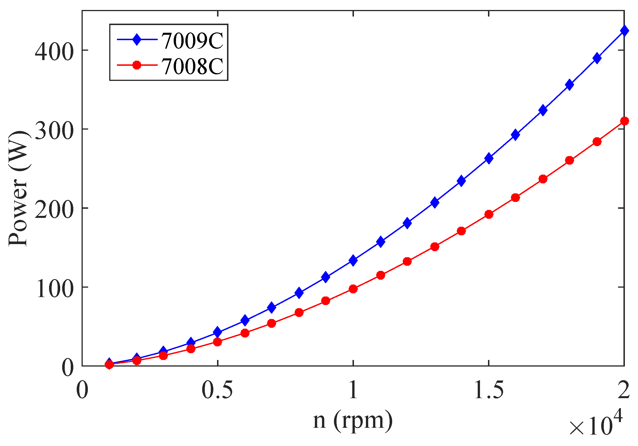
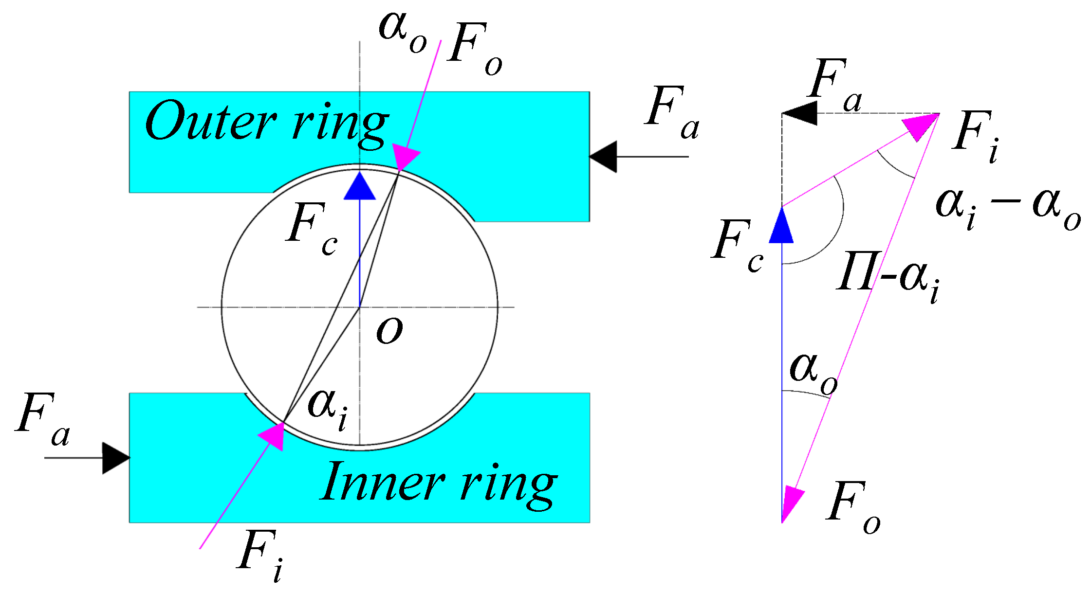
2.1. Bearing Heating Power
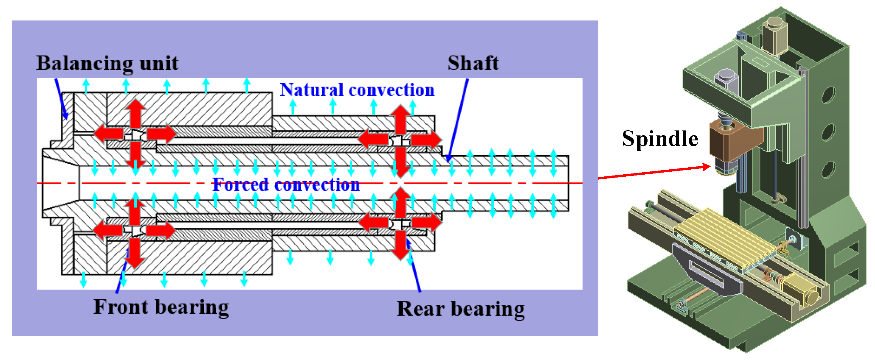
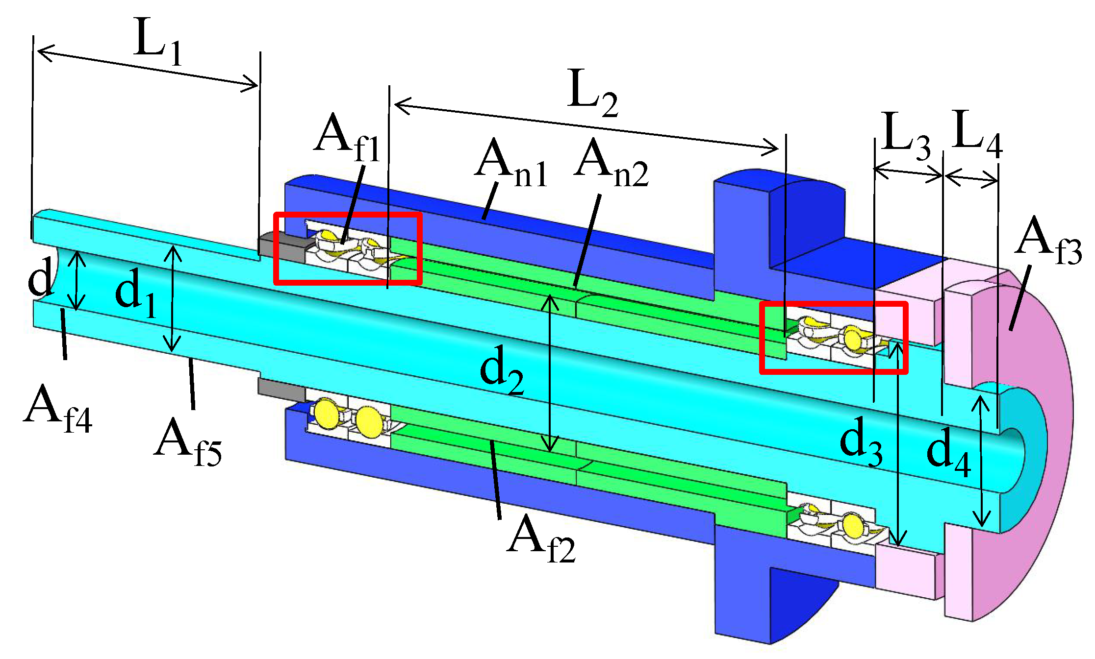
2.2. CHTCs of Spindle
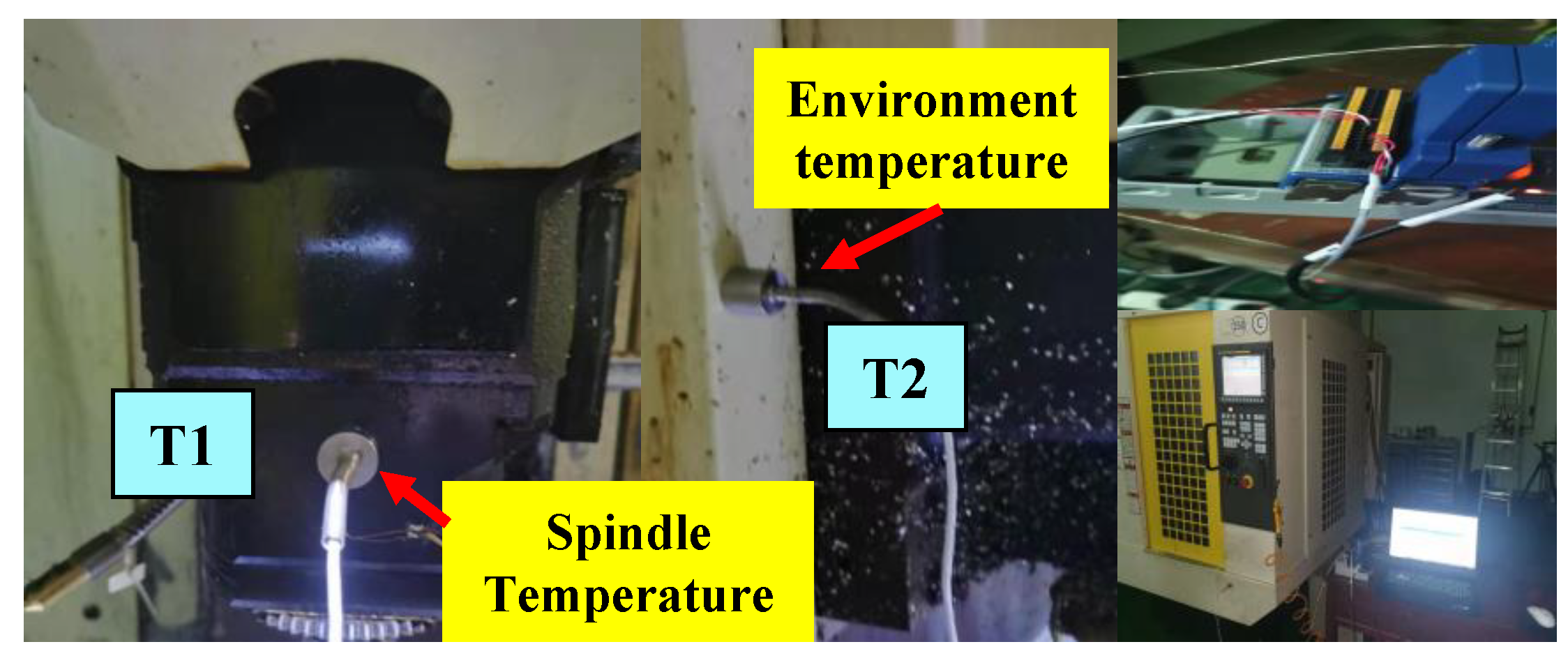
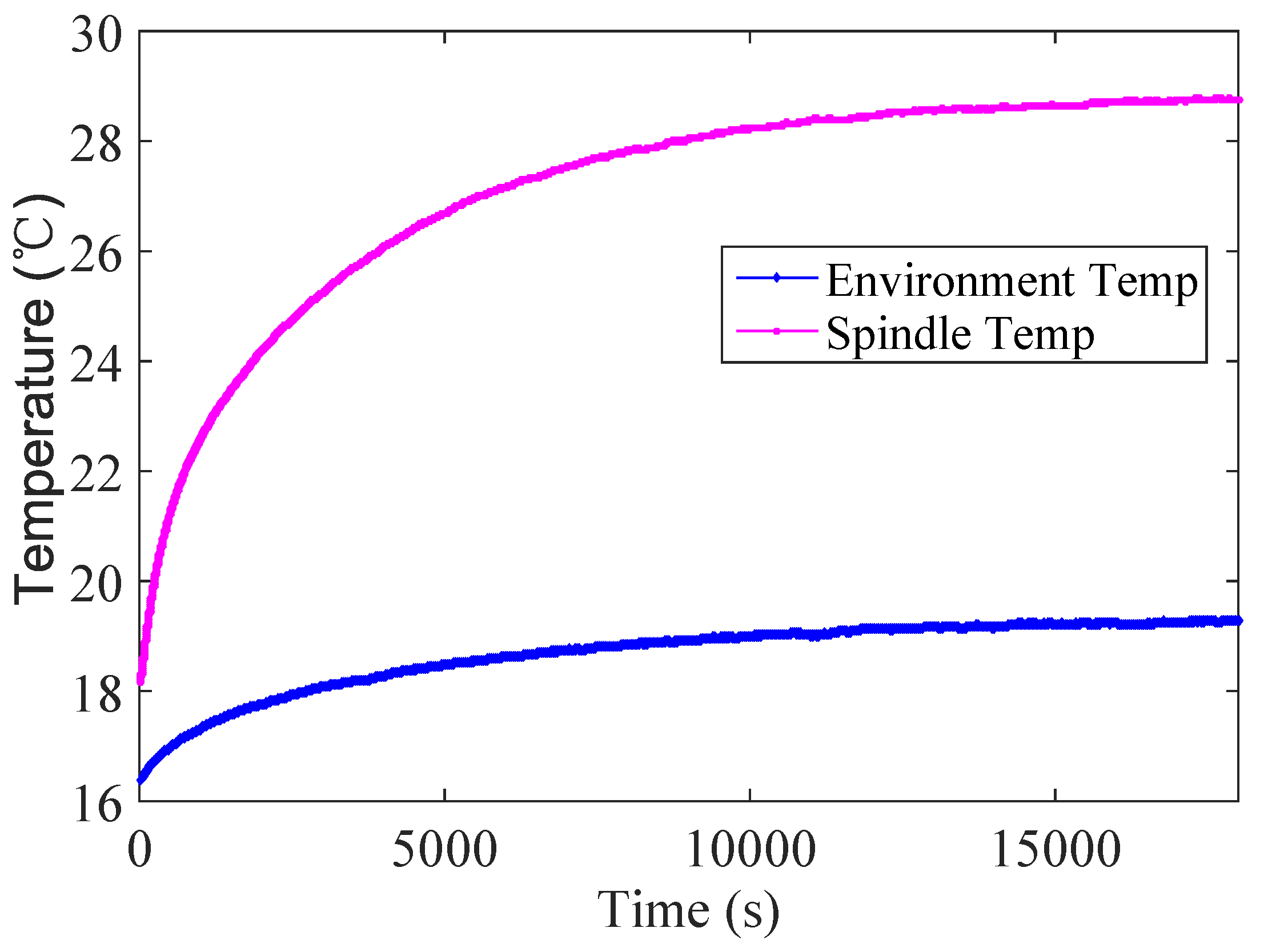
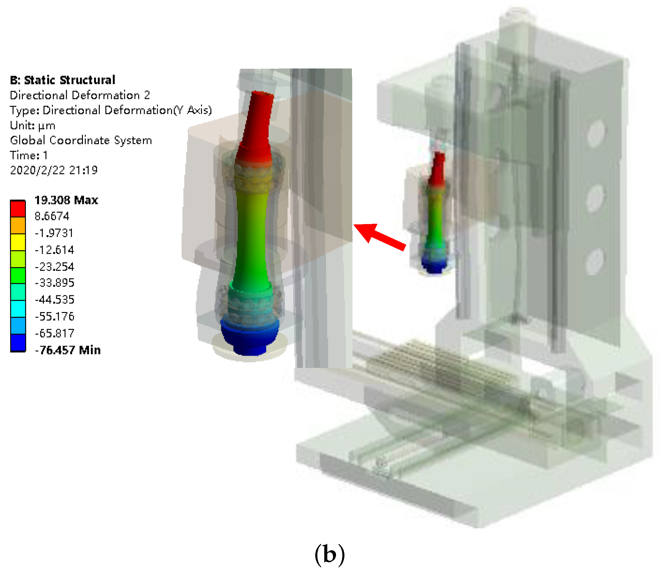
2.3. Thermal Experiment and Finite Element Thermal Analysis (FETA)
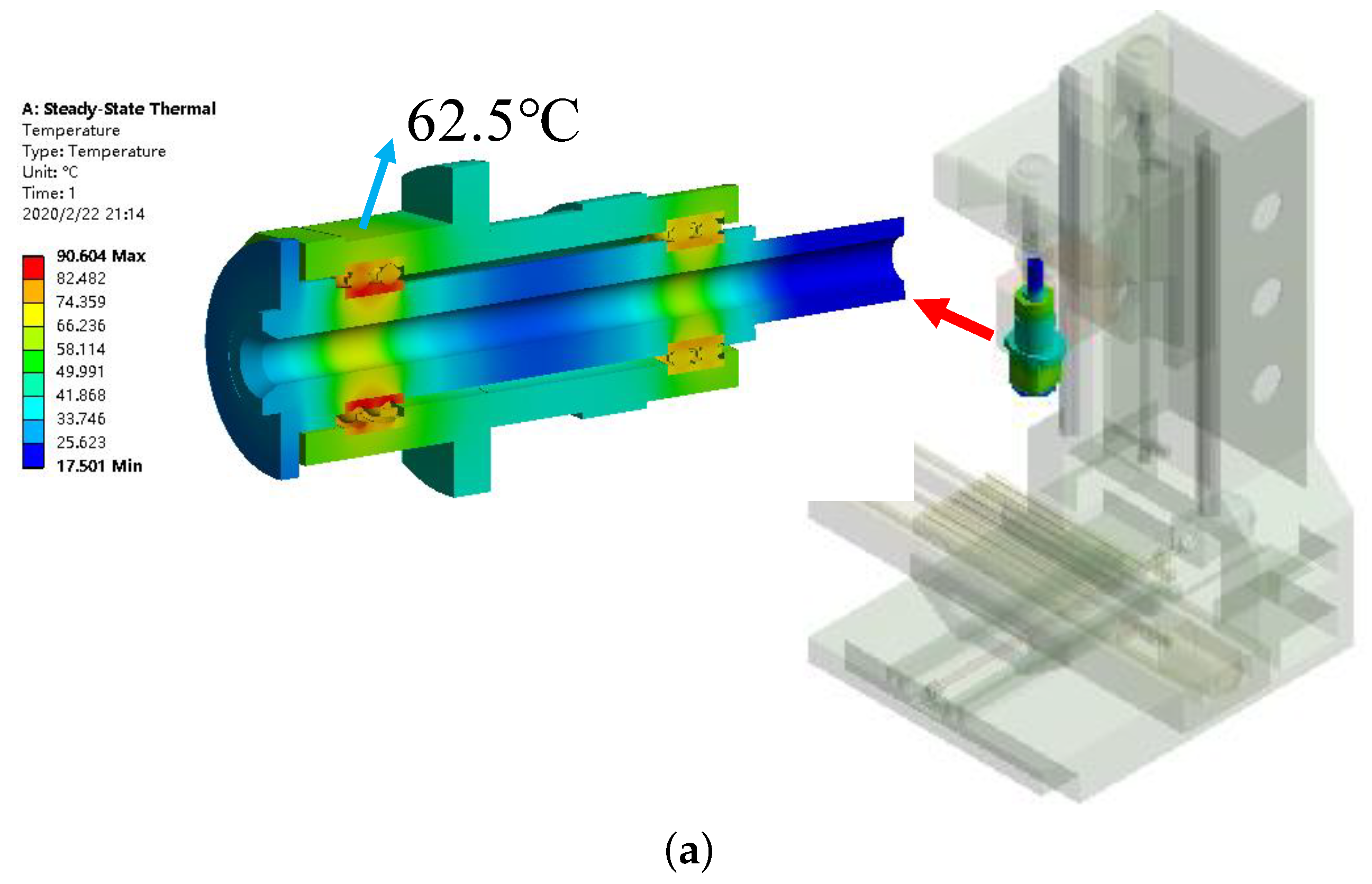
2.4. FETA Results
3. Optimization of Thermal Boundary Parameters
- (1)
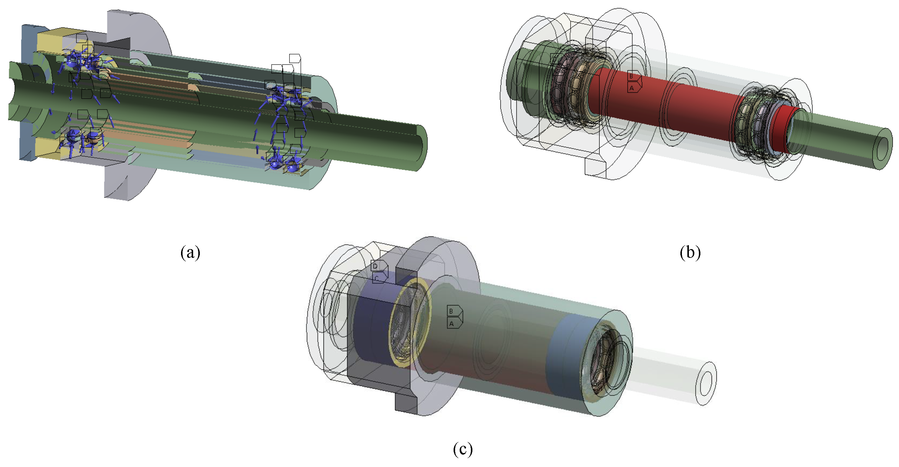
- Establishing the simplified digital model of spindle unit based on the design parameters and meshing it.
- (2)
- Setting the TBCs according to simplified empirical formula, such as bearing heat power, thermal contact resistances between the contact surfaces, and CHTCs of the spindle units’ surfaces. The ambient temperature is 17.5 C, and spindle rotating speed is 20,000 rpm.
- (3)
- According to the simulation error, correct the TBCs based on an RSM hybrid ABC algorithm.
- (4)
- Then, the optimized TBCs are substituted to the FEM for analysis and compared with the experimental results.
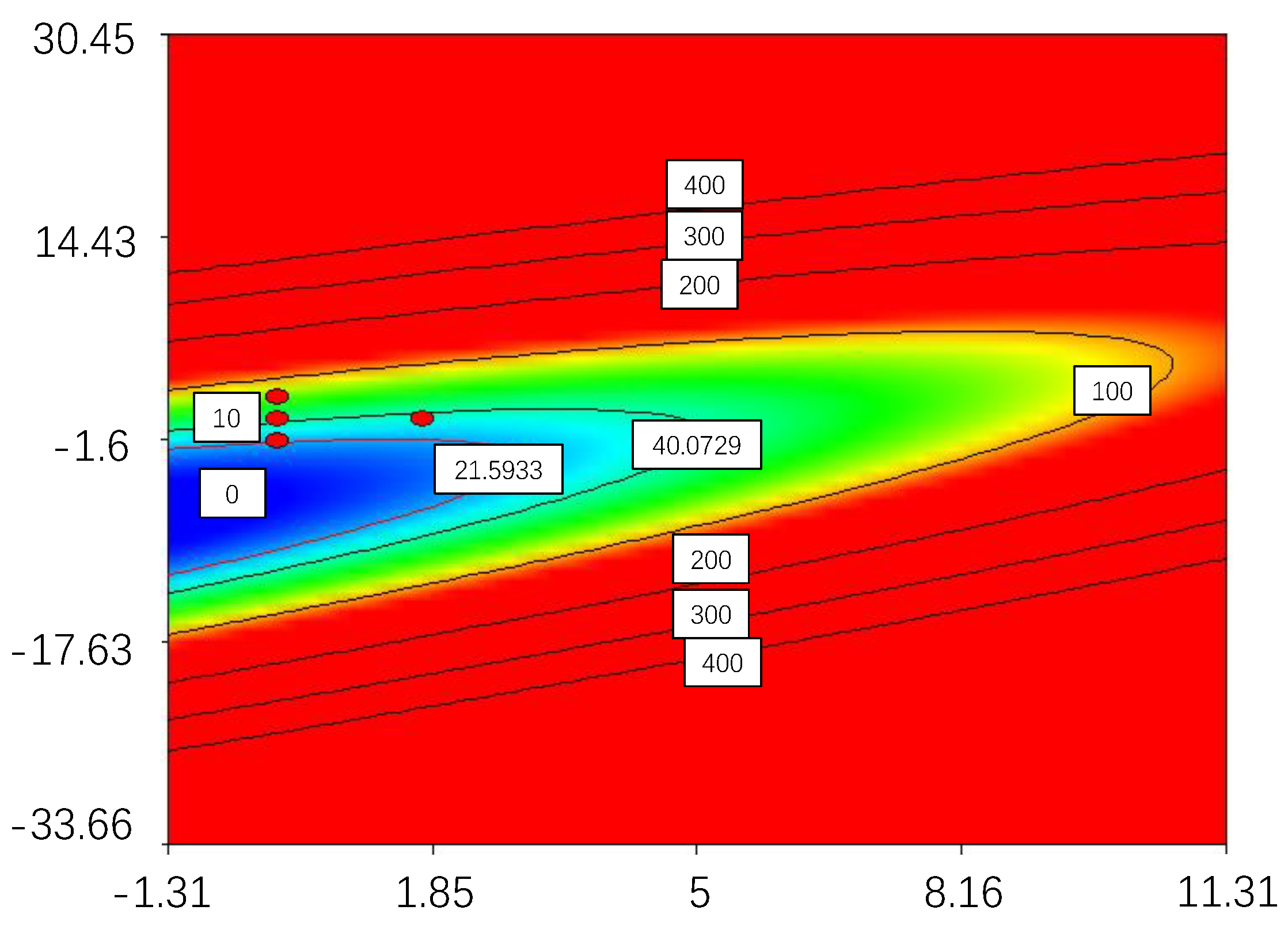
3.1. DE and RSM
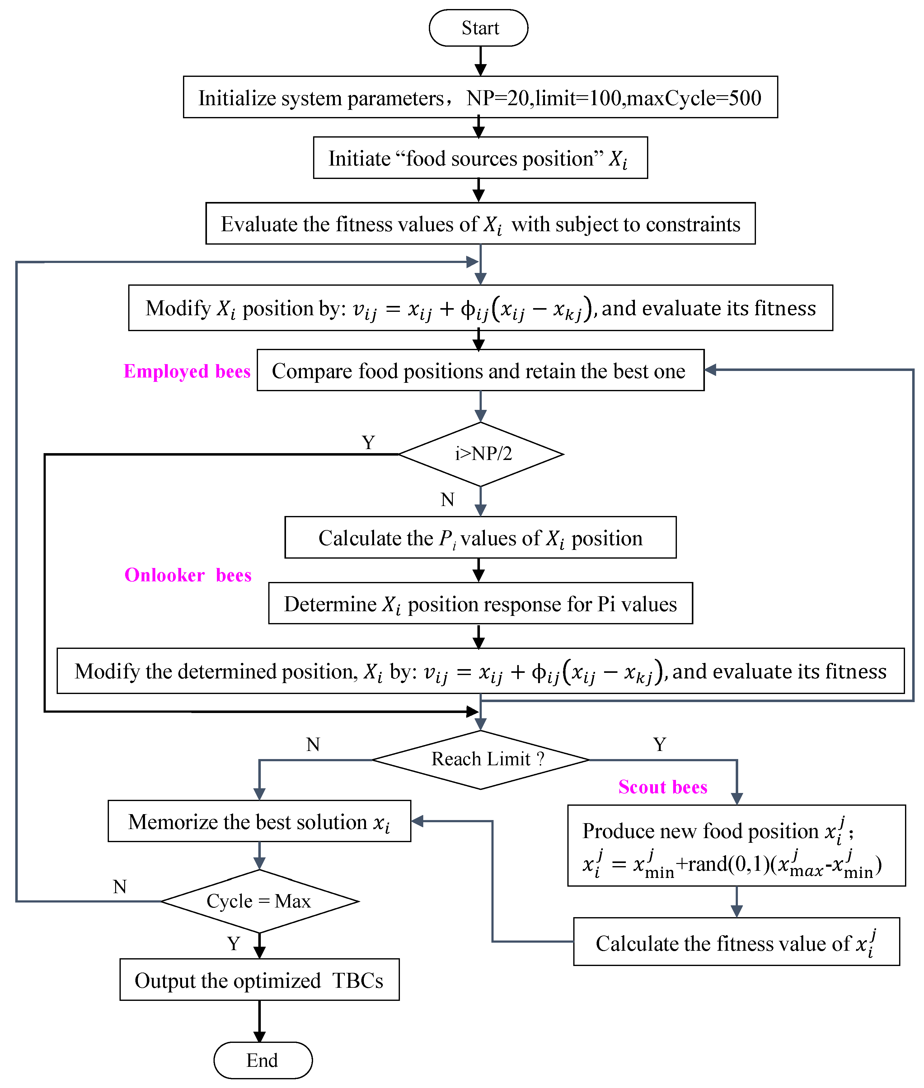
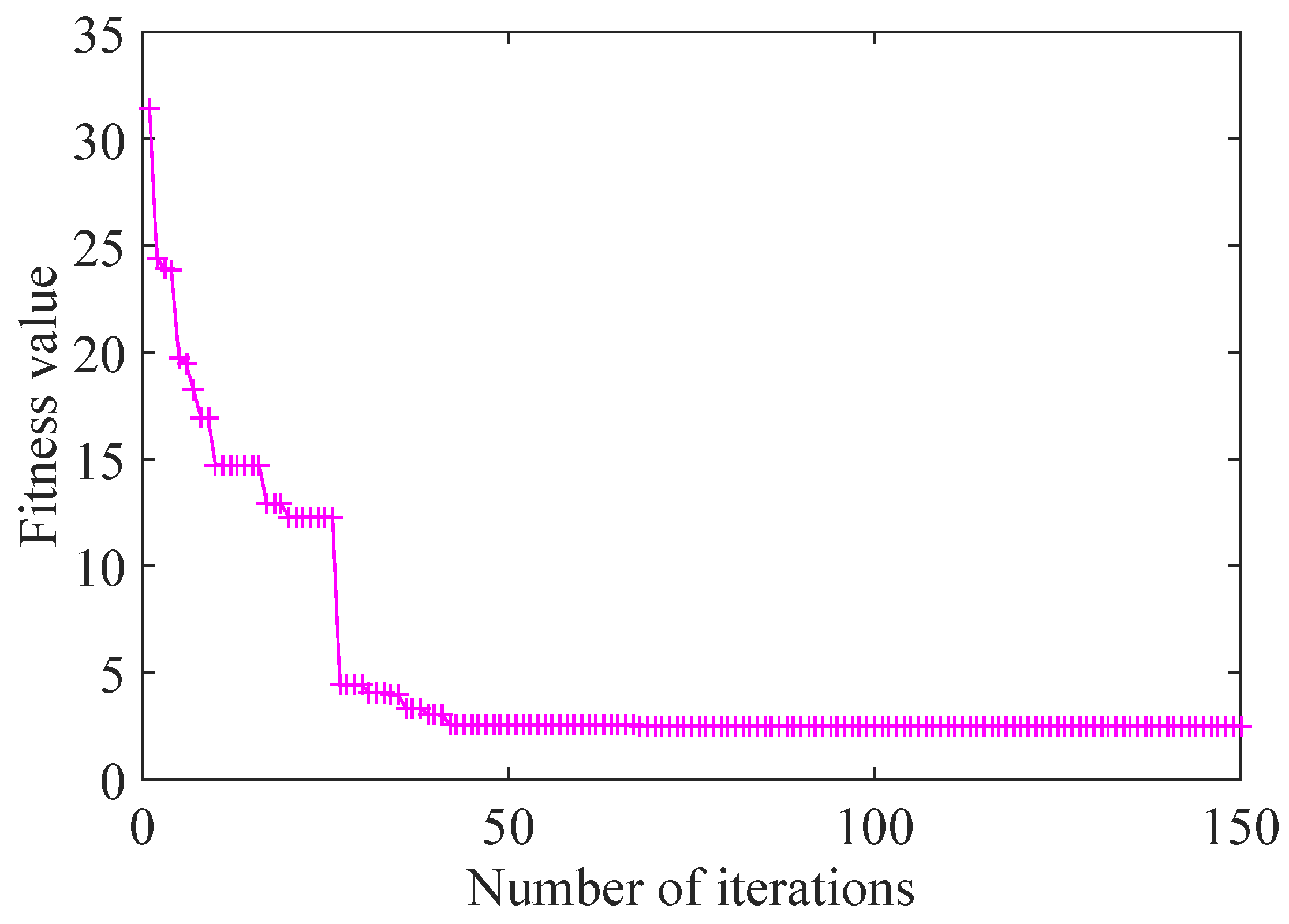
3.2. ABC
4. Comparison of FEA Results of Spindle before and after Optimization
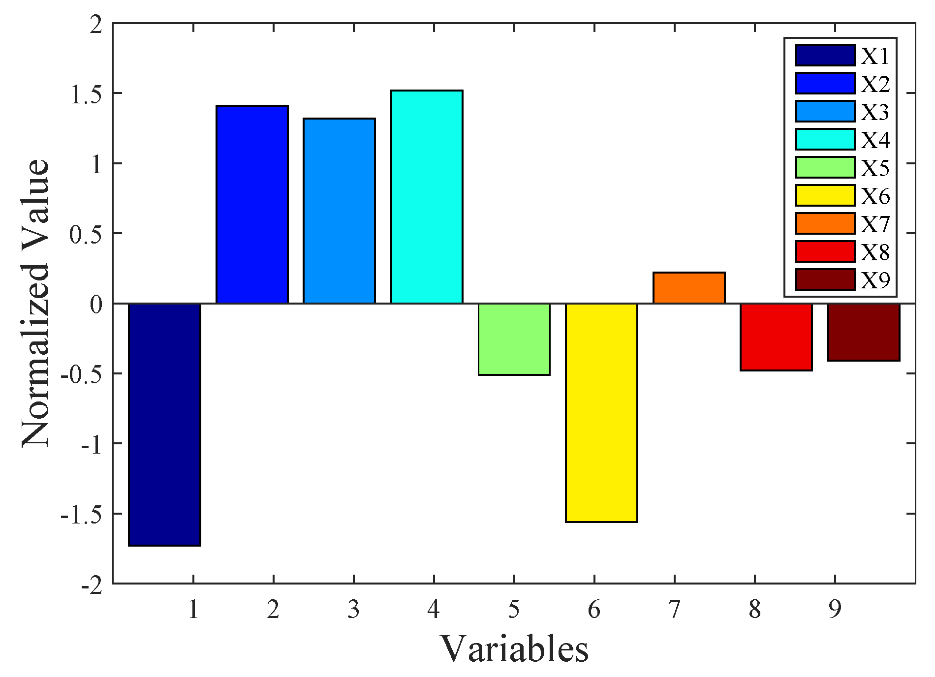
4.1. The Optimized TBCs
- Step1: Initialize system parameters and the population of solutions , and = [ ]
- Step2: Evalute the population, which is to take the value of into and compare the fitness value.
- Step3: Cycle = 1
- Step4: repeat
- Step5: Produce new solutions ti for the employed bees by using and evaluate them
- Step6: Apply the greedy selection process for the employed bees.
- Step7: Calculate the probability values for the solutions by .
- Step8: Produce the new solutions for the onlookers from the solutions selected depending on and evaluate them.
- Step9: Apply the greedy selection process for the onlookers.
- Step10: Determine the abandoned solution for the scout, if it exists, and replace it with a new randomly produced solution by .
- Step11: Memorize the best solution achieved so far.
- Step12: cycle = cycle + 1.
- Step13: until cycle = MCN.
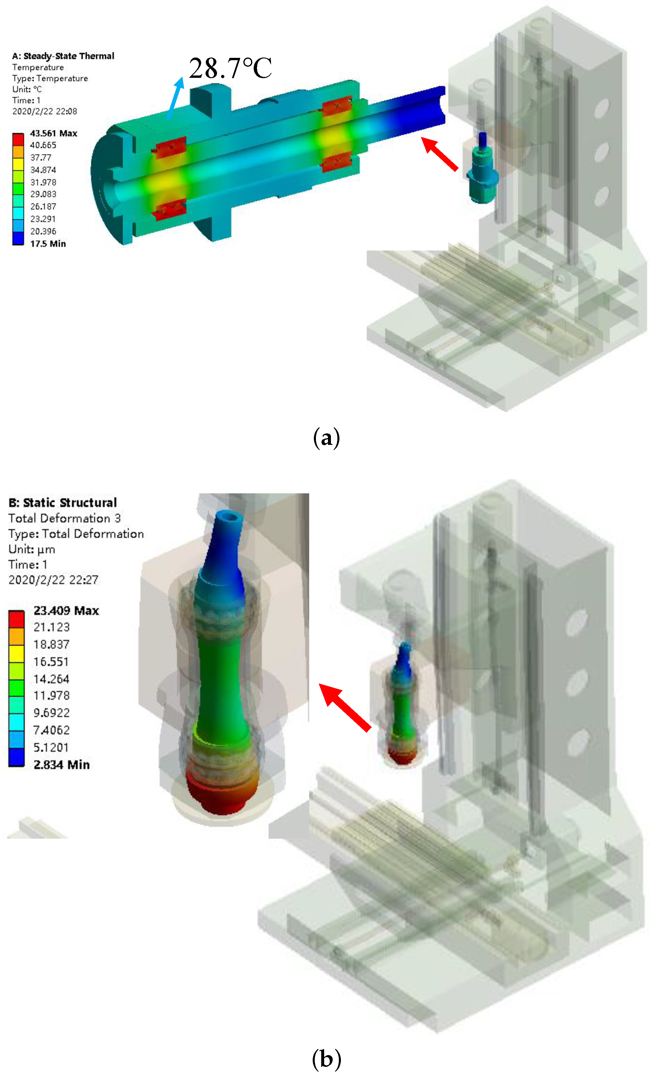
4.2. Comparision of Finite Element Thermal Analysis Results
5. Conclusions
Author Contributions
Funding
Conflicts of Interest
References
- Jedrzejewski, J.; Kwasny, W. Modelling of angular contact ball bearings and axial displacements for high-speed spindles. CIRP Ann. 2010, 59, 377–382. [Google Scholar] [CrossRef]
- Kim, J.D.; Zverv, I.; Lee, K.B. Thermal model of high-speed spindle units. KSME Int. J. 2003, 2, 10. [Google Scholar] [CrossRef]
- Yan, B.; Yan, K.; Luo, T.; Zhu, Y.; Li, B.Q.; Hong, A.J. Thermal coefficients modification of high speed ball bearing by multi-object optimization method. Int. J. Therm. Sci. 2019, 137, 313–324. [Google Scholar] [CrossRef]
- Li, Y.; Zhao, W.; Lan, S.; Ni, J.; Wu, W.; Lu, B. A review on spindle thermal error compensation in machine tools. Int. J. Mach. Tools Manuf. 2015, 95, 20–38. [Google Scholar] [CrossRef]
- Liu, H.; Miao, E.; Zhuang, X.; Wei, X. Thermal error robust modeling method for cnc machine tools based on a split unbiased estimation algorithm. Precis. Eng. 2018, 51, 169–175. [Google Scholar] [CrossRef]
- Li, Q.; Li, H.L. A general method for thermal error measurement and modeling in cnc machine tools’ spindle. Int. J. Adv. Manuf. Technol. 2019, 103, 2739–2749. [Google Scholar] [CrossRef]
- Liu, K.; Liu, Y.; Sun, M.; Li, X.; Wu, Y. Spindle axial thermal growth modeling and compensation on cnc turning machines. Int. J. Adv. Manuf. Technol. 2016, 87, 2285–2292. [Google Scholar] [CrossRef]
- Haitao, Z.; Jianguo, Y.; Jinhua, S. Simulation of thermal behavior of a cnc machine tool spindle. Int. J. Mach. Tools Manuf. 2007, 47, 1003–1010. [Google Scholar] [CrossRef]
- Liu, Z.; Pan, M.; Zhang, A.; Zhao, Y.; Yang, Y.; Ma, C. Thermal characteristic analysis of high-speed motorized spindle system based on thermal contact resistance and thermal conduction resistance. Int. J. Adv. Manuf. Technol. 2014, 76, 1913–1926. [Google Scholar] [CrossRef]
- Ma, C.; Yang, J.; Zhao, L.; Mei, X.; Shi, H. Simulation and experimental study on the thermally induced deformations of high-speed spindle system. Appl. Therm. Eng. 2015, 86, 251–268. [Google Scholar] [CrossRef]
- Chen, G.C.; Wang, L.Q.; Le, G.U.; Zhen, D.Z. Heating analysis of the high speed ball bearing. J. Aerosp. Power 2007, 22, 163–168. [Google Scholar]
- Harris, T.A.; Kotzalas, M.N. Rolling Bearing Analysis, 5th ed.; CRC/Taylor & Francis: Boca Raton, FL, USA, 2007. [Google Scholar]
- Li, Y.; Zhao, W.; Wu, W.; Lu, B. Boundary conditions optimization of spindle thermal error analysis and thermal key points selection based on inverse heat conduction. Int. J. Adv. Manuf. Technol. 2016, 90, 2803–2812. [Google Scholar] [CrossRef]
- Zhang, L.; Gong, W.; Zhang, K.; Wu, Y.; An, D.; Shi, H.; Shi, Q. Thermal deformation prediction of high-speed motorized spindle based on biogeography optimization algorithm. Int. J. Adv. Manuf. Technol. 2018, 97, 3141–3151. [Google Scholar] [CrossRef]
- Tan, F.; Wang, L.; Yin, M.; Yin, G. Obtaining more accurate convective heat transfer coecients in thermal analysis of spindle using surrogate assisted differential evolution method. Appl. Therm. Eng. 2019, 149, 1335–1344. [Google Scholar] [CrossRef]
- Fu, C.B.; Tian, A.H.; Yau, H.T.; Hoang, M.C. Thermal monitoring and thermal deformation prediction for spherical machine tool spindles. Therm. Sci. 2019, 23, 2271–2279. [Google Scholar] [CrossRef]
- Li, Y.; Wei, W.M.; Su, D.X.; Zhao, W.H.; Zhang, J.; Wu, W.W. Thermal error modeling of spindle based on the principal component analysis considering temperature-changing process. Int. J. Adv. Manuf. Technol. 2018, 99, 1341–1349. [Google Scholar] [CrossRef]
- Yin, Q.; Tan, F.; Chen, H.X.; Yin, G.F. Spindle thermal error modeling based on selective ensemble bp neural networks. Int. J. Adv. Manuf. Technol. 2019, 101, 1699–1713. [Google Scholar] [CrossRef]
- Liu, T.; Gao, W.G.; Zhang, D.W.; Zhang, Y.F.; Chang, W.F.; Liang, C.M.; Tian, Y.L. Analytical modeling for thermal errors of motorized spindle unit. Int. J. Mach. Tools Manuf. 2017, 112, 53–70. [Google Scholar] [CrossRef]
- Incropera, F.P. Fundamentals of Heat and Mass Transfer; John Wiley Sons: Hoboken, NJ, USA, 2011. [Google Scholar]
- Yan, K.; Hong, J.; Zhang, J.; Mi, W.; Wu, W. Thermal-deformation coupling in thermal network for transient analysis of spindle-bearing system. Int. J. Therm. Sci. 2016, 104, 1–12. [Google Scholar] [CrossRef]
- Jiang, S.Y.; Mao, H.B. Investigation of variable optimum preload for a machine tool spindle. Int. J. Mach. Tools Manuf. 2010, 50, 19–28. [Google Scholar] [CrossRef]
- Jedrzejewski, J.; Kowal, Z.; Kwasny, W.; Modrzycki, W. High-speed precise machine tools spindle units improving. J. Mater. Process. Technol. 2005, 162, 615–621. [Google Scholar] [CrossRef]
- Hinkelmann, K.; Kempthorne, O. Principles of Experimental Design; Wiley: Hoboken, NJ, USA, 2007. [Google Scholar]
- Galtchouk, L.I. On sequential estimation of parameters for linear regression with martingale noise. In MODA 5 Advances in Model-Oriented Data Analysis and Experimental Design; Atkinson, A.C., Pronzato, L., Wynn, H.P., Eds.; Physica-Verlag HD: Heidelberg, Germany, 1998; pp. 105–114. [Google Scholar]
- Yang, J.; Honavar, V.G. Feature Subset Selection Using a Genetic Algorithm; Springer: Boston, MA, USA, 1998. [Google Scholar]
- Gozali, A.A.; Fujimura, S. Localization Strategy for Island Model Genetic Algorithm to Preserve Population Diversity; Computer and Information Science; Springer: Cham, Switzerland, 2018. [Google Scholar]
- Pant, M.; Thangaraj, R.; Abraham, A. A New PSO Algorithm with Crossover Operator for Global Optimization Problems; Springer: Berlin/Heidelberg, Germany, 2007. [Google Scholar]
- Karaboga, D.; Akay, B. A comparative study of artificial bee colony algorithm. Appl. Math. Comput. 2009, 214, 108–132. [Google Scholar] [CrossRef]
- Karaboga, D.; Basturk, B. A powerful and efficient algorithm for numericial function optimization: Artificial bee colony (abc) algorithm. J. Glob. Optim. 2007, 39, 459–471. [Google Scholar] [CrossRef]


| Bearing Type | 7008C | 7009C |
|---|---|---|
| (kN) | 15.9 | 19.3 |
| (mm) | 54 | 60 |
| Preload force (N) | 290 | 340 |
| Spindle Speed (rpm) | Heat Transfer Coefficients (W/mC) | (W) | (W) | ||||||
|---|---|---|---|---|---|---|---|---|---|
| 2000 | 42.2 | 43.3 | 44.0 | 32.8 | 40.6 | 9.7 | 9.7 | 6.8 | 9.2 |
| 4000 | 66.4 | 68.3 | 69.7 | 52.1 | 64.5 | 9.7 | 9.7 | 21.3 | 29.2 |
| 6000 | 85.4 | 89.4 | 91.4 | 68.3 | 84.5 | 9.7 | 9.7 | 41.8 | 57.2 |
| 8000 | 102.3 | 108.3 | 110.7 | 82.7 | 102.4 | 9.7 | 9.7 | 67.5 | 92.4 |
| 10,000 | 123.3 | 126.6 | 128.4 | 95.9 | 118.8 | 9.7 | 9.7 | 97.7 | 133.8 |
| 12,000 | 139.2 | 143 | 145.2 | 108.3 | 134.2 | 9.7 | 9.7 | 132.4 | 181.3 |
| 14,000 | 154.4 | 158.5 | 160.8 | 120 | 148.7 | 9.7 | 9.7 | 171.1 | 234.4 |
| 16,000 | 168.7 | 173.3 | 175.7 | 131.3 | 162.6 | 9.7 | 9.7 | 213.6 | 292.7 |
| 18,000 | 182.5 | 187.4 | 190 | 142 | 175.8 | 9.7 | 9.7 | 259.9 | 356.1 |
| 20,000 | 195.8 | 201 | 203.9 | 152.3 | 188.6 | 9.7 | 9.7 | 309.7 | 424.4 |
| Joint Surface | Thermal Resistance (mC/W) |
|---|---|
| Bearing inner ring/shaft | |
| Bearing outer ring/housing | |
| Rolling elements/raceways | |
| Other contact surfaces |
| Spindle Structure (45) | Bearing (GCr15) | Bearing (Coolants (air)) | |
|---|---|---|---|
| Density (kg/m) | 7800 | 8000 | 1.1796 |
| Thermal conductivity (W·mK) | 60.5 | 40.1 | 1.0069 |
| Young’s Modulus (GPa) | 210 | 200 | − |
| Poisson’s ratio | 0.28 | 0.3 | − |
| Linear expansion coefficient (K | 1.2 × | 1.3 × | − |
| Temperature Points | Experimental (C) | Simulated (C) | Error (C) | Error (%) |
|---|---|---|---|---|
| T1 | 27.4 | 62.5 | 35.1 | 128.1 |
| Number | −1.732 | −1 | 0 | 1 | 1.732 |
|---|---|---|---|---|---|
| 33.4 | 55.4 | 85.4 | 115.4 | 137.4 | |
| 37.4 | 59.4 | 89.4 | 119.4 | 141.4 | |
| 22.1 | 51.4 | 91.4 | 131.4 | 160.7 | |
| 16.3 | 38.3 | 68.3 | 98.3 | 120.3 | |
| 15.2 | 44.5 | 84.5 | 124.5 | 153.8 | |
| 1 | 4.7 | 9.7 | 14.7 | 18.4 | |
| 1 | 4.7 | 9.7 | 14.7 | 18.4 | |
| 7.2 | 21.8 | 41.8 | 61.8 | 76.4 | |
| 5.2 | 27.2 | 57.2 | 87.2 | 109.2 |
| Number | Design Variable (Normalized) | |||||||||
|---|---|---|---|---|---|---|---|---|---|---|
| 1 | 1 | 1 | 1 | −1 | 1 | 1 | 1 | −1 | 1 | 36.2 |
| 2 | −1 | 1 | −1 | −1 | 1 | 1 | 1 | −1 | 1 | 26.9 |
| · | · | · | · | · | · | · | · | · | · | · |
| 155 | −1 | 1 | −1 | −1 | −1 | 1 | 1 | 1 | 1 | 38.6 |
| 156 | 1 | −1 | 1 | 1 | −1 | −1 | −1 | 1 | −1 | 22.2 |
| Temperature Points | Experimental (C) | Simulated (C) | Error (C) | Error (%) |
|---|---|---|---|---|
| T1 | 27.4 | 28.7 | 1.3 | 4.7 |
© 2020 by the authors. Licensee MDPI, Basel, Switzerland. This article is an open access article distributed under the terms and conditions of the Creative Commons Attribution (CC BY) license (http://creativecommons.org/licenses/by/4.0/).
Share and Cite
Zhang, L.; Xuan, J.; Shi, T. Obtaining More Accurate Thermal Boundary Conditions of Machine Tool Spindle Using Response Surface Model Hybrid Artificial Bee Colony Algorithm. Symmetry 2020, 12, 361. https://doi.org/10.3390/sym12030361
Zhang L, Xuan J, Shi T. Obtaining More Accurate Thermal Boundary Conditions of Machine Tool Spindle Using Response Surface Model Hybrid Artificial Bee Colony Algorithm. Symmetry. 2020; 12(3):361. https://doi.org/10.3390/sym12030361
Chicago/Turabian StyleZhang, Leilei, Jianping Xuan, and Tielin Shi. 2020. "Obtaining More Accurate Thermal Boundary Conditions of Machine Tool Spindle Using Response Surface Model Hybrid Artificial Bee Colony Algorithm" Symmetry 12, no. 3: 361. https://doi.org/10.3390/sym12030361
APA StyleZhang, L., Xuan, J., & Shi, T. (2020). Obtaining More Accurate Thermal Boundary Conditions of Machine Tool Spindle Using Response Surface Model Hybrid Artificial Bee Colony Algorithm. Symmetry, 12(3), 361. https://doi.org/10.3390/sym12030361