Article

Rapid Identification and Prediction of Cadmium-Lead Cross-Stress of Different Stress Levels in Rice Canopy Based on Visible and Near-Infrared Spectroscopy

1
State Key Laboratory of Information Engineering in Surveying, Mapping and Remote Sensing, Wuhan University, Wuhan 430079, China
2
School of Resource and Environmental Sciences, Wuhan University, Wuhan 430079, China
3
Department of Urban Planning and Design, The University of Hong Kong, Hong Kong 999077, China
*
Author to whom correspondence should be addressed.
Remote Sens. 2020, 12(3), 469; https://doi.org/10.3390/rs12030469
Submission received: 4 December 2019 / Revised: 23 January 2020 / Accepted: 27 January 2020 / Published: 2 February 2020

Abstract

:
Accurate detection of cadmium (Cd) and lead (Pb)-induced cross-stress on crops is essential for agricultural, ecological environment, and food security. The feasibility to diagnose and predict Cd–Pb cross-stress in agricultural soil was explored by measuring the visible and near-infrared reflectance of rice leaves. In this study, two models were developed—namely a diagnostic model and a prediction model. The diagnostic model was established based on visible and near-infrared reflectance spectroscopy (VNIRS) datasets with Support Vector Machine (SVM), followed by leave-one-out cross-validation (LOOCV). A partial least-squares (PLS) regression, as the prediction model was employed to predict the foliar concentration of Cd and Pb contents. To accurately calibrate the two models, a rigorous greenhouse experiment was designed and implemented, with 4 levels of treatments on each of the Cd and Pb stress on rice. Results show that with the appropriate pre-processing, the diagnostic model can identify 79% of Cd and 85% of Pb stress of any levels. The significant bands that have been used mainly distributed between 681–776 nm and 1224–1349 nm for Cd stress and 712–784 nm for Pb stress. The prediction model can estimate Cd with coefficient of determination of 0.7, but failed to predict Pb accurately. The results illustrated the feasibility to diagnose Cd stress accurately by measuring the visible and near-infrared reflectance of rice canopy in a cross-contamination soil environment. This study serves as one step forward to heavy metal pollutant detection in a farmland environment.

Graphical Abstract

1. Introduction

Over recent decades, the accumulation of heavy metals in agricultural soil has been an important issue worldwide related to environmental pollution and human risk [1]. Distinguishing the types and levels of heavy metals in agricultural soil is of crucial importance for food safety and health risks, which does help to prevent and curb heavy metal pollution. Therefore, it is necessary to detect and quantify heavy metal contaminations in agricultural soil.
Conventionally, the spatial distribution of heavy metals in agricultural soil was usually analyzed by numerous field samplings and subsequent chemical analyses in the laboratory, followed by geo-statistical interpolation [2,3], which was low-efficiency and time-consuming. Moreover, due to the limited information at certain locations and moments, it could not be used to describe the spatial and temporal dynamics of heavy metal concentrations over large areas [4].
VNIRS (350 nm to 2500 nm) is a highly efficient and non-destructive tool for ecological applications, which allows qualitative and quantitative analysis to be implemented in different matrices. Thus, it can be used, not only to estimate soil properties by soils hyperspectral reflectance, such as clay [5], moisture [6], organic matter [4,7,8] and iron oxides [9], but to estimate heavy metals concentration by soils hyperspectral spectra, such as Pb [4,10,11], Cd [7,10,12], zinc (Zn) [7,13], copper (Cu) [9,13,14], mercury (Hg) [15,16] and so on, in agricultural soils.
In terms of the diagnosis of heavy metals, intensive studies investigated the mechanisms and feasibility based on VNIRS. Liu et al. [17] investigated the feasibility of using hyperspectral data after wavelet-fractal analysis to monitor the polluted levels of rice with heavy metal pollution. Shi et al. [18] explored the mechanism of why, with VNIRS, we are able to monitor limited types of heavy metal contamination in soils and tried to diagnose the Arsenic contamination in agricultural soils [19]. Chen et al. [12] investigated the feasibility of using VNIRS to identify soil Cd pollution risk. Diagnostic techniques are essentially Boolean classification models, including random forests (RF) [19], wavelet-fractal analysis [20], a support vector machine (SVM) [21] and an artificial neural network (ANN) [19], which have been commonly applied in previous studies. However, these methods were often implemented in diagnosis of single heavy metal pollution [22,23], and a few studies took corresponding contaminative diagnosis with different stress levels into consideration, especially the diagnosis of a common polluted phenomenon with Cd–Pb cross-stress in paddy fields [24,25,26].
In terms of prediction of heavy metals, first in 1997, VNIRS was used to estimate accurately heavy metal concentrations in soil [27]. Hereafter, some similar studies were performed in various regions, such as mining areas [14,28,29], floodplains [4,7,30], deltas [16,31,32], and suburban areas [33]. In recent years, more and more studies, especially in China, have focused on estimating concentrations of heavy metals in agricultural soils [13,34,35]. Among the predicted models, there were principle component regression (PCR) [36], BPNN [37], linear regression model [4], stepwise multiple linear regression (SMLR) [15], a genetic algorithm-based stacking algorithm [38] and a memory-based learning approach [39]. However, partial least-squares regression (PLSR) was considered to be a common standard tool to relate wavebands to biochemical contents with the optimal function by minimizing the error of sum squares [5,13,34,40,41]. Several recent studies have also indicated the feasibility of using PLSR to predict heavy metal contents in soils [13,34,42].
In the abovementioned studies, most involved the diagnosis and prediction of only a single heavy metal. When involving multiple heavy metals, a traditional wet chemical analysis was often needed. A few studies have tried to diagnose and predict the cross-stress caused by contamination with multiple heavy metals on the basis on the hyperspectral datasets in canopy.
The major objective of this study was to investigate the feasibility of diagnosing and predicting Cd–Pb cross-stress based on rice canopy hyperspectral data by the efficient and environmentally friendly VNIRS. To the best of our knowledge, this is the first study identifying and predicting Cd–Pb cross-stress by using VNIRS. The specific objectives of the current work were to: (1) acquire hyperspectral datasets of rice canopy stressed by Cd–Pb cross-stress with four different stress levels, ranging from 350 nm to 2500 nm; (2) establish discrimination models to diagnose the types and the stress levels and investigate the diagnostic ability between single pretreatments and combined pretreatments and (3) establish prediction models to predict the Cd–Pb contents in rice leaf.

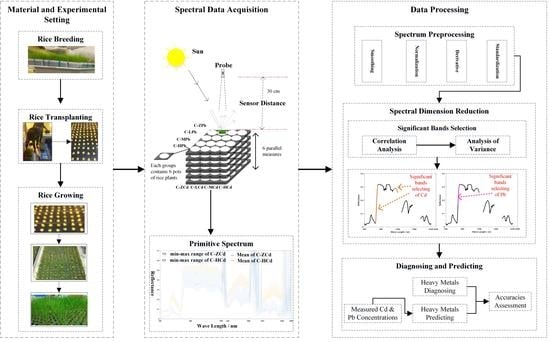
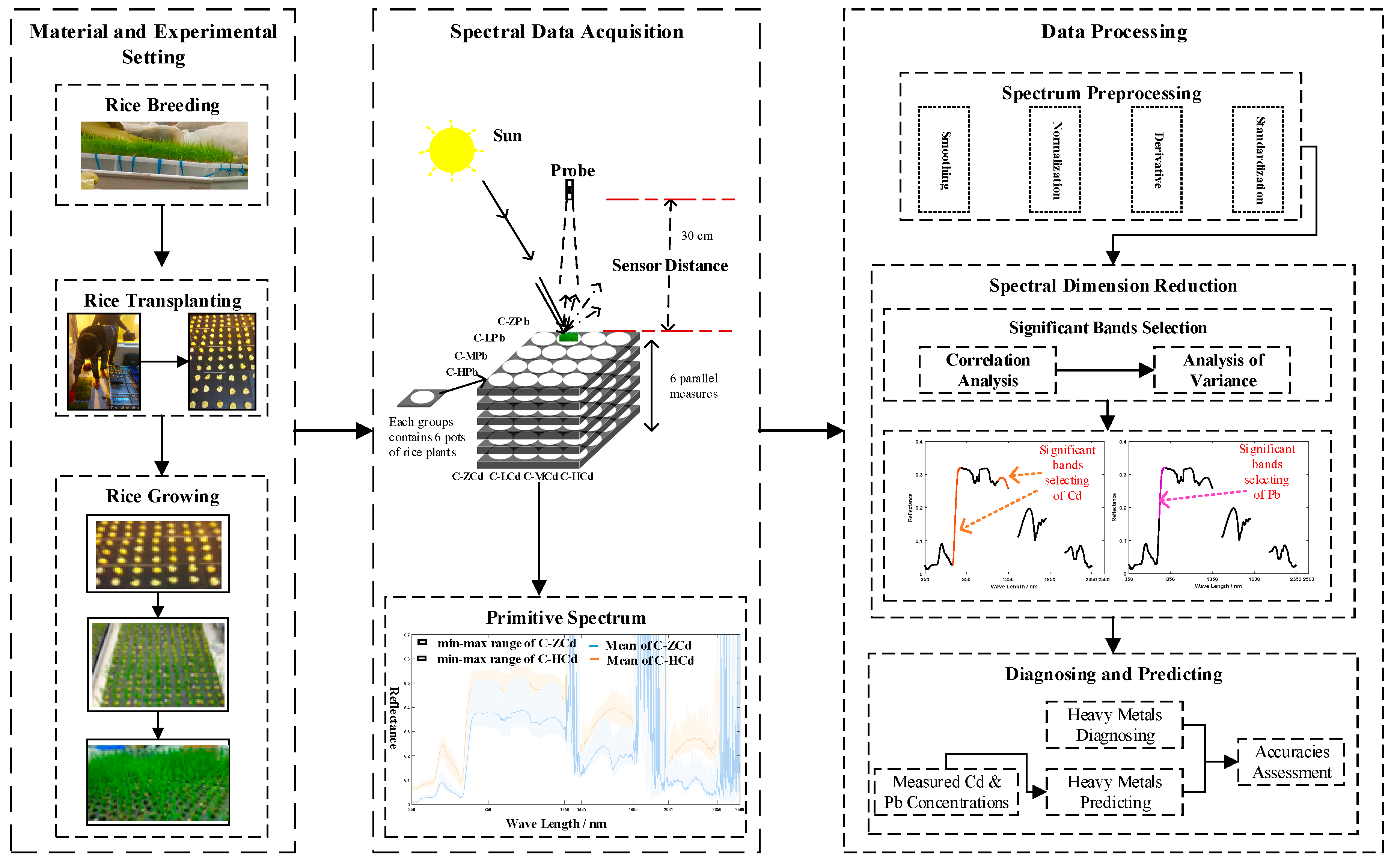
2. Materials and Methods

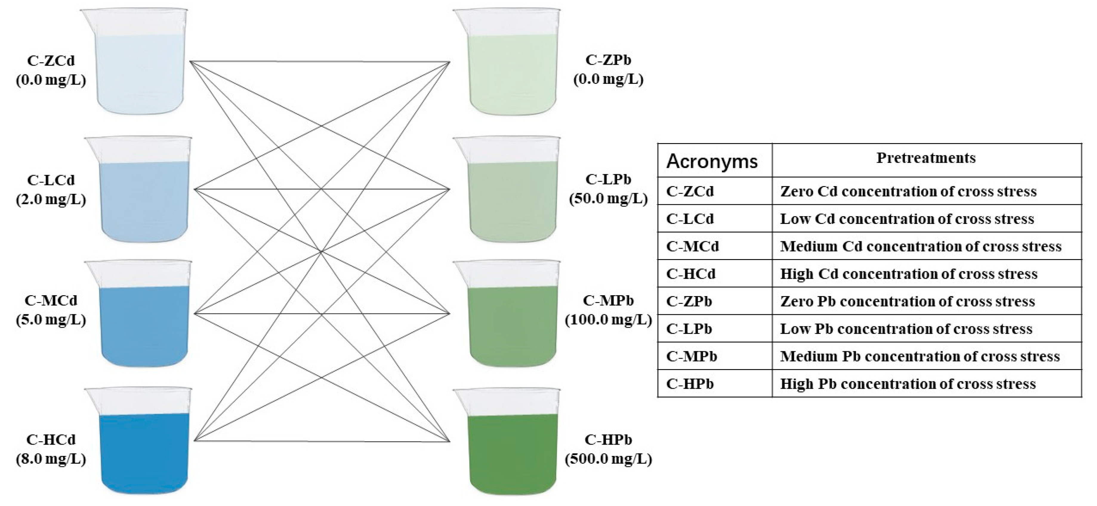
2.1. Experimental Design

Rice was employed to be an indicator of heavy metal pollution in farmland, due to its extensive planting in the vast areas of China and Southern India. Thanks to serious pollution, Cd and Pb were selected to be the polluted types [43,44]. To effectively control the environmental variables, such as temperature, humidity, and light, the experiment was carried out in a glass greenhouse with a stable temperature of 25–30 °C and a humidity of 60–80%. The greenhouse has a ceiling that can be opened and closed by a switch. 576 pots of rice were planted in hydroponics and will be assigned to 96 groups, with 6 pots per group. The stress levels of heavy metals could be accurately controlled during the experiment. The nutrient solution recommended by the International Rice Research Institute was used as the basic rice hydroponic solution, while cadmium chloride (CdCl2) and lead nitrate (Pb(NO3)2) were used as the solute to regulate Cd and Pb contents in nutrient solution. solid plastic boxes with painted black were used as the containers for nutrient solution, and black foam boards with holes were used as fixed supports for rice seedlings above the boxes. These nutrient solutions with different Cd–Pb concentrations were replaced every ten days to ensure the rice was not under the other stress due to poor nutrient ingredients.
We designed a Cd–Pb cross stressed experiment with four different stress levels by referencing the controlled concentrations in farmland in GB15618-2018 of China [45]. The four different stress levels were 0 mg/L, 2 mg/L, 5 mg/L and 8 mg/L of Cd and 0 mg/L, 50 mg/L, 100 mg/L and 500 mg/L of Pb, and then, there were, totally, 16 groups with different combinations. The detailed concentrations, corresponding abbreviations and the combinations are showed in Figure 1. In the following statement, the abbreviations were going to be used to represent the corresponding treatments. The experimental process is showed in Figure 2.

2.2. Spectrum and Cd–Pb Contents in Leaf Measurement

The spectral reflectance data of the rice canopy were measured inside the greenhouse with ceiling opened, by a FieldSpec3 portable spectroradiometer (Analytical Spectral Devices, Inc., USA) at 10:00–14:00 local time, under cloud-free or near-cloudless weather conditions [17,46]. The spectral instrument covers the VNIRS region from 350 nm to 2500 nm with two different spectral resolutions: 3 nm for 350–1000 nm and 10 nm for 1000–2500nm, respectively.
At the late booting stages of rice, each group of rice were sampled for the reflective spectra of their canopy. At this stage, when measured from nadir direction at 30 cm height, there are roughly 90% of foliar tissue and 10% dark background within the field-of-view. Spectra were acquired with 8 averages of slightly different centering points of the samples. Spectral measurements were calibrated with a white standard reference panel, resulting in 96 reflective spectra for the 96 groups of rice canopy.
After the spectral measurement, these rice leaves were collected in groups and refrigerated in the laboratory with the temperature of 16–18 °C. In the lab, rice leaves were ground to homogenate and digested for later use. The linear regression equation of the relationship between absorbance and concentration was found by blank test. Under the same conditions, an equal amount of sample solution was put into the graphite furnace to measure the absorbance value; the above linear equation was taken to obtain the sample Cd/Pb contents. The Cd/Pb contents in the sample was calculated as follows:
X =   ( c 1 c 0 ) × V m × 1000
where C1 and C0 are the Cd/Pb contents with a unit of ng/mL in the digestive solution and the blank control solution, respectively, while v is the total volume of the sample digestive solution with a unit of Ml and m is the mass of the sample with a unit of g.

2.3. Spectral Pre-Processing

To reduce the random error of sampling randomly, the spectral means of eight randomly selected measured spots in same stress pre-processing were calculated in the MATLAB 2015a platform, and then the calculated values were used as the spectrum for the corresponding stress treatments of single acquisition. As a result, there were a total of 96 spectra, each group containing six. To decrease instrument noises and to improve the signal-to-noise ratio, the spectral bands (1351–1460 nm, 1801–2030 nm and 2351–2500 nm) were removed from calculated reflectance spectra, and the remaining hyperspectral datasets were processed by the following pretreatments:
Derivative pretreatment, including first derivative and second derivative, eliminated the interferences of background noise, resolved overlapping spectra, and minimized additive baseline drift of raw spectral reflectance [18]. Savitzky–Golay smoothing [47] was applied to remove random noise and to increase spectral data quality. Normalization and standardization decreased redundant information and extracted the spectral difference, which did help to remove unnoticeable weight. Besides the above single pre-processing methods, we tried to combine two or more single pretreatment methods together, and took the priority of pre-processing methods into consideration to find appropriate combinations to improve diagnostic accuracies [19]. As a result, the study employed 10 different pretreatments.
Table 1 displayed the pre-processing methods employed in this study and their corresponding abbreviations. In the combined pre-processing methods, the order of abbreviations represented the priority of pre-processing methods. Take NorSG1D as an example. The abbreviation represented first normalization, then Savitzky–Golay smoothing followed by 1st-Derivative.

2.4. Spectral Dimension Reduction

(Two-way analysis of variance) ANOVA was performed to extract significant bands from spectral variables for Cd–Pb cross-stress. Analysis of variance was used to test the difference between multiple means to determine whether a stressed factor had a significant effect on the spectral changes. ANOVA was applied to discriminate the factors of spectral change in a certain band, and these factors included Cd stress, Pb stress, and conjunct stress. These bands with spectral changes that were only related to one stressed factor were selected to be used as the significant bands. By comparing the significance value with a preset confidence (p = 0.05), the corresponding bands with lower value than the preset significance value were selected as significant band for subsequent diagnosis and prediction.

2.5. Model Calibration

2.5.1. Diagnosis of Heavy Metals

SVM transfers training data into a higher-dimensional feature space using a kernel function and then computes separating hyperplanes as a result of achieving maximum separation between the classes [48]. It is often used to diagnose and classify the hyperspectral datasets with a small scale. In this study, an SVM with the linear kernel function was employed to diagnose the levels of Cd–Pb cross-stress. By pre-training, the optimal combination of parameters was determined.

2.5.2. Prediction of Cd–Pb Contents

PLSR is often preferred to quantitatively derive information from hyperspectral reflectance spectra [8]. When calculating the principal components, PLSR is more interpretable, and it is the more efficient algorithm than PCR in relating the selected significant bands to heavy metals contents. PLSR associates the partial least-squares (PLS) method with a classical multivariate linear regression to explain the correlation between the selected significant bands from VNIRS datasets and the Cd–Pb contents:
y ^ = X · b ^ + b 0
where X ϵ R M , N is a matrix of M spectra samples with N spectral bands, y ^ R M , 1 is the vector of the predicted Cd or Pb values of the M rice leaf samples, b ^ R N , 1 is the vector of the estimated PLSR regression coefficients (b-coefficients) and b 0 is the intercept [49].
Significant bands in different pretreatment methods were used as independent variables to predict Cd–Pb contents in the leaves of rice. For each prediction, two thirds of hyperspectral samples were randomly selected as calibration dataset, and one third remaining samples were treated as test dataset. The model with the best evaluation performance was selected as the final model.
SVM is also widely used for its robust prediction tasks. This paper adopts SVMs with radial basis kernel function. The hidden node is the inner product of the input sample and a support vector, and the output node is the linear combination of the hidden layer output. The input variables of the prediction model are the pre-processed significant bands. The output target value is the predicting concentration of contaminations. Finally, accuracy of prediction was calculated against those of PLSR. Method with higher performance is employed in this study.

2.6. Model Evaluation

2.6.1. Diagnostic Models Evaluation

Leave-one-out cross-validation was employed to evaluate the diagnostic performance of SVM model in the study, whereby each hyperspectral dataset was diagnosed by remaining datasets [50]. By this way, it provided nearly unbiased predictions even with the limitation of sample numbers [51]. For 96 hyperspectral samples total, the diagnostic model was run 96 times, and the mean of 96 diagnostic results was regarded as the accuracies of diagnostic model.

2.6.2. Predictive Models Evaluation

The prediction models, created between the heavy metal (Cd and Pb) contents and spectral variables, were evaluated based on the coefficient of determination ( r 2 ), the root mean squared error (RMSE) and the ratio of the interquartile distance of measured values to RMSE (RPIQ) [52,53], which were given by:
r 2 = 1 i = 1 N ( y i y i ) 2 / i = 1 N ( y i y ¯ ) 2
R M S E = i = 1 N ( y i y i ) 2 N
RPIQ = I Q / S E P
where y i and y i are the measured and predicted values of the Cd/Pb contents, and y ¯ is the average measured value and N is the hyperspectral sample number. By analyzing the predicted performance of all significant bands, the predicted results with the highest r 2 would be used as the final prediction model. IQ is the interquartile distance, and SEP represents the standard error of prediction.

3. Results

3.1. Leaf Cd–Pb Contents

The statistical descriptions of leaf Cd–Pb contents for the whole data sets, calibration data sets, and validation data sets are shown in Table 2. These statistical characters, such as mean and standard deviation (SD), were similar to three data sets with a small difference. These characteristic similarities indicated that the randomly selected calibration and validation data sets could effectively represent the whole data sets.

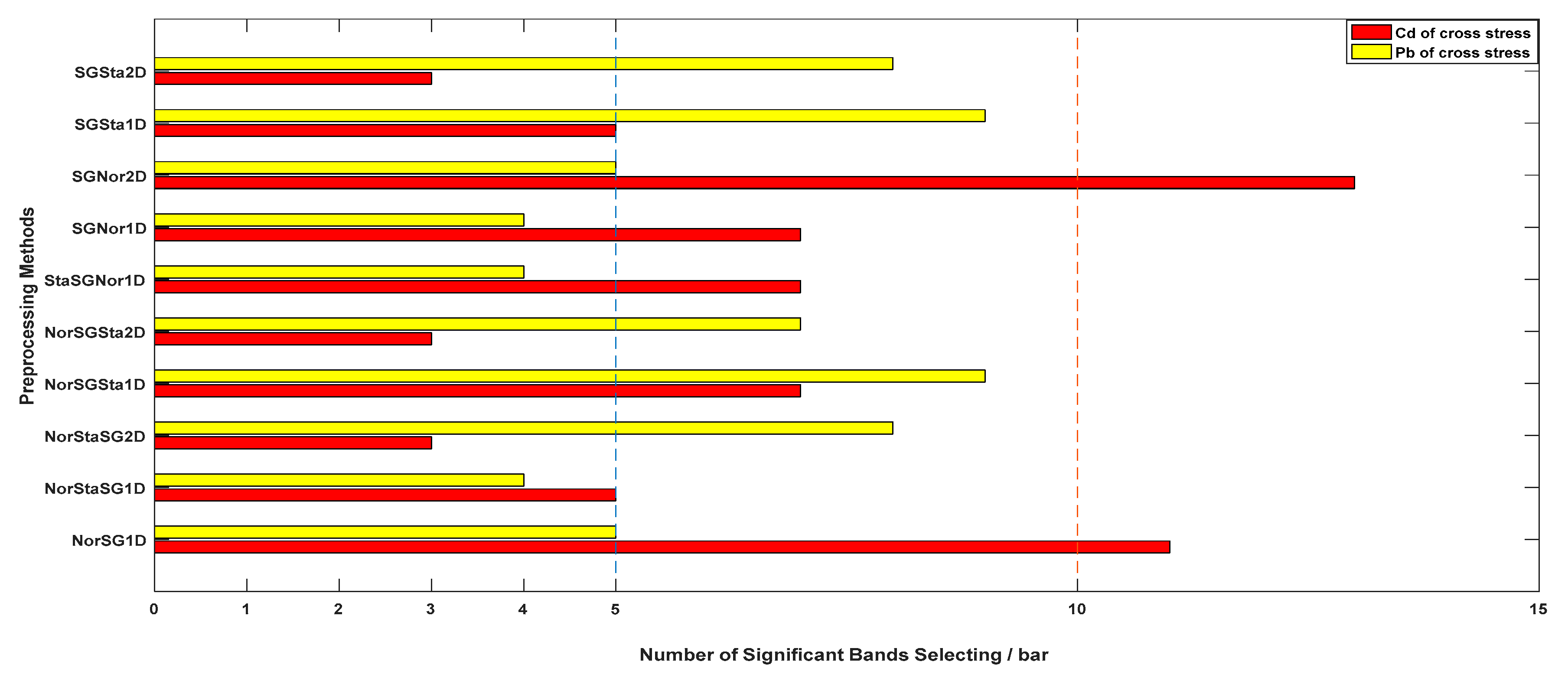
3.2. Significant Bands

The numbers of significant bands varied with different pretreatment methods for Cd and Pb, as displayed in Figure 3.
The number of significant bands selected for Pb stress was no more than 10 in any pretreatment with the most bands of nine, while the most pre-processing methods for Cd stress were less than 10 with the most bands of 13. The minimum number of significant bands for Cd and Pb were 3 and 4, respectively, which could not be selected by the same pre-processing method.
For Cd, half of pretreatments could select the significant bands with no more than 5, three of which have selected the 3, including NorStaSG2D, NorSGSta2D, and SGSta2D. Like Cd, there were three pre-processing methods that selected the minimum number of four for Pb stress, such as NorStaSG1D, StaSGNor1D, and SGNor1D, as illustrated in Figure 3.

3.3. Spectral Response to Single Contamination

In Figure 4, the ranges of significant bands for Cd (a) and Pb (b), and the foliar spectral responses to different level of Cd (c) and Pb (d) in these spectral ranges were plotted.
Significant bands detected with ANOVA for Cd-stressed are mainly distributed in the two extents of 681–776 nm and 1224–1349 nm, while that for Pb-stressed were concentrated distribution in the range from 712 nm to 784 nm. The Cd–Pb spectral response showed reverse patterns. With the increasing concentration of Cd, the foliar reflectance generally increases except the extent at 681–699 nm, while with the increasing concentration of Pb, the reflectance generally drops. However, this pattern is not applicable to the reflectance of unpolluted plants. Apart from the main ranges of significant bands, plotted in Figure 4, there were some bands to scatter at 1461 nm for Cd and 815 nm, 1280–1281 nm, 1476 nm, and 1601 nm. The foliar reflectance characteristics of these scatted significant bands showed the same pattern with the corresponding contaminative heavy metals.

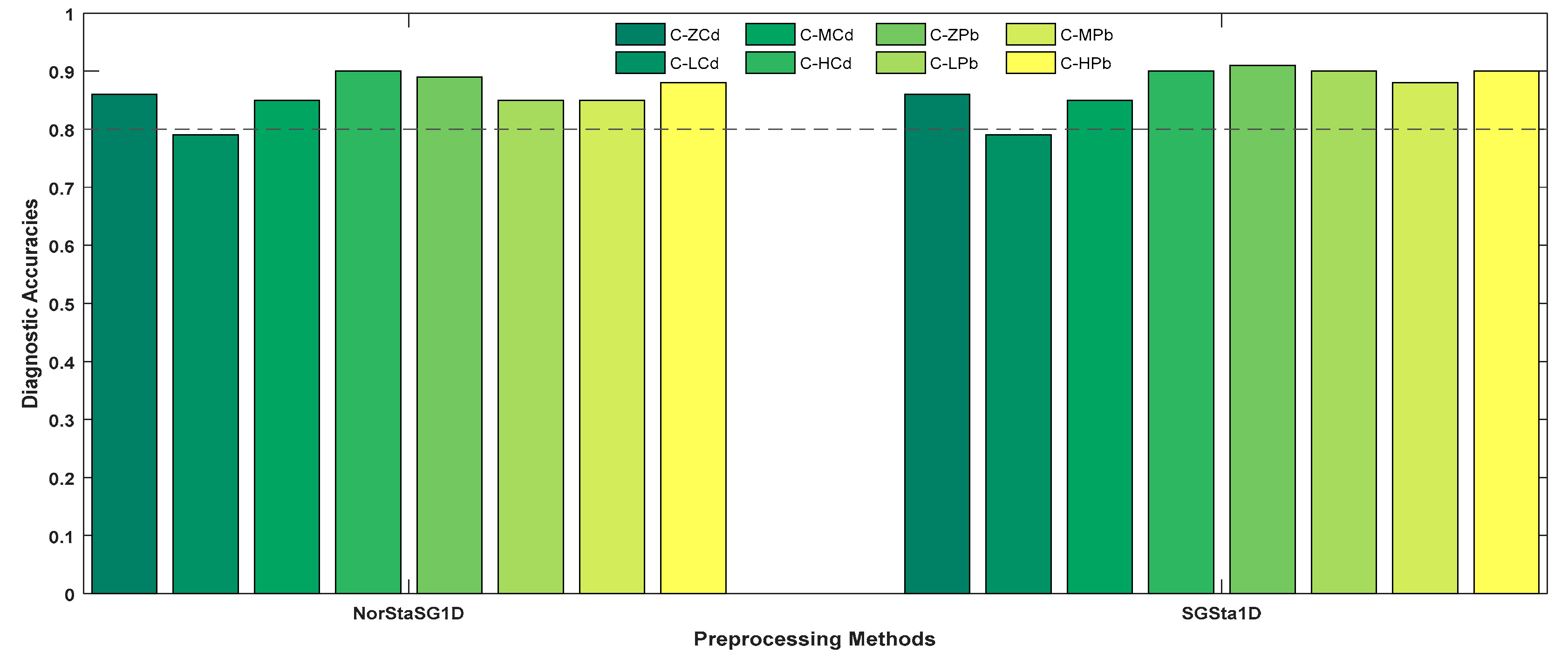
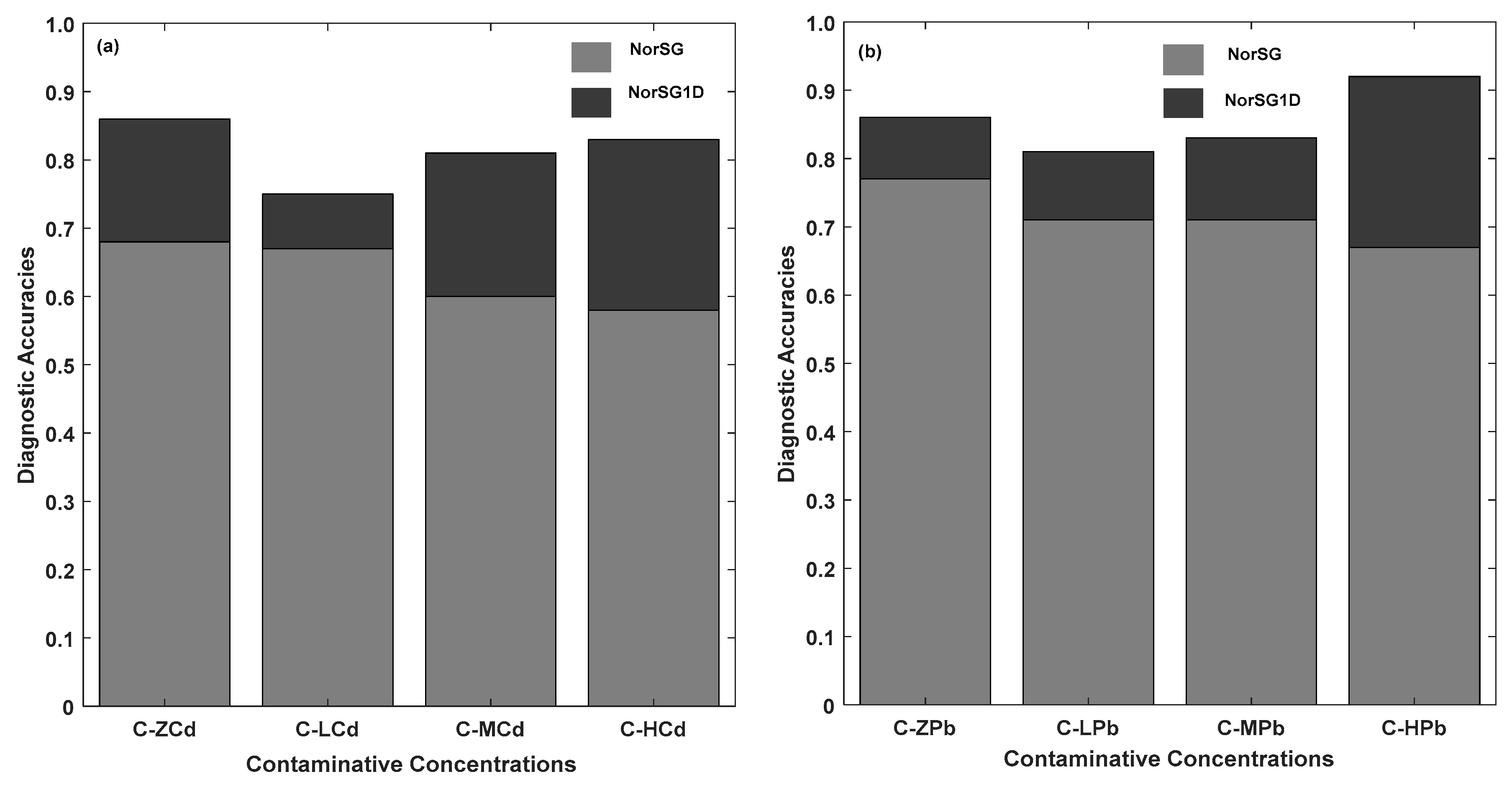
3.4. Diagnosis of Cd–Pb Cross-Stress with Different Stress Levels

All pre-processing methods were employed one by one for the selection of significant bands and for the further diagnosis of the specific stress levels that the rice was subject to. Based on the preset diagnostic labels, the selected significant bands were input to the SVM diagnostic model to distinguish specific stress levels and other stress levels, and the overall accuracies were the output diagnostic accuracies. Take the diagnosis of zero-Pb stress level (C–ZPb) as an example. As shown in Table 3, there was a total of 96 samples, including 24 zero-Pb stress level samples and 72 other stress levels samples. Based on pretreatment of NorStaSG1D, 21 zero-Pb stress level samples and 64 other stress level samples were diagnosed correctly, and total 85 samples were diagnosed with the correct stress level and as a result, the overall accuracy was 0.89.
The complete diagnostic accuracies were showed in Table 4. When only a single pretreatment was employed, the accuracies reached 0.60. When three or more pretreatment methods were combined, the diagnostic accuracies boosted to more than 0.8. The bolds represented that the diagnostic accuracy in any stress level was not less than 0.75 and 0.85 for Cd and Pb, respectively.
All diagnostic accuracies reached 0.75 for all pretreatments. The accuracies of Cd-stressed levels ranged from 0.75 to 0.90, with the highest of 0.90 for C–HCd. The accuracies of Pb-stressed levels ranged from 0.79 to 0.92. The highest accuracy was 0.91 for C–HPb.
For Cd stress in cross-stress, all pretreatments that reached accuracies of not less than 0.75 no matter what Cd-stressed levels the rice was subject to. Especially there were three pretreatments with an accuracy of not less than 0.79, including NorStaSG1D, SGNor2D, and SGSta1D. Based on the pretreatments of SGNor2D, all accuracies reached 0.81 in any Cd stress level. When diagnosing whether the rice was subject to zero-Cd stress level (C–ZCd), accuracies ranged from 0.81 to 0.86 from different pre-processing reflective spectra. the highest accuracy was 0.86 based on the four pretreatments, including NorSG1D, NorStaSG1D, SGNor1D, and SGSta1D.; for low-Cd stress level (C–LCd), the overall diagnostic accuracies were distributed in the range from 0.75 to 0.81, and the highest accuracy was 0.81 based on the significant bands of SGNor2D. Half of pretreatments reached diagnostic accuracies of not less than 0.77, which was a greatly acceptable result; for medium-Cd stress level (C–MCd), the accuracies exceeded 0.80except SGSta2D at 0.79. its highest value reached 0.90 in the pretreatment of SGNor1D;; for high-Cd stress level (C–HCd), half of pretreatments reached a diagnostic accuracy of no less than 0.85, which indicated that any of them could diagnose C–HCd from four stress levels in cross-stress. There were three pretreatments that reached 0.90, including NorStaSG1D, SGNor1D, and SGSta1D.
For Pb stress in cross-stress, among all pretreatments, there were six pretreatments that reached accuracies of not less than 0.85, no matter what Pb-stressed levels the rice was subject to. Especially for NorSGSta1D and SGSta1D, the diagnostic accuracies were not less than 0.88 in any Pb stress level. When diagnosing whether the rice was subject to zero-Pb stress level (C–ZPb), and the diagnostic accuracies ranged from 0.86 to 0.91 from different pre-processing reflective spectra, four of which reached 0.88. The highest was 0.91 based on the pretreatment of NorSGSta1D and SGSta1D. for medium-Pb stress level (C–MPb), the overall diagnostic accuracies were distributed to the extent of 0.81 to 0.90. with more than half of the pretreatments, these corresponding diagnostic accuracies were not less than 0.85, and the highest accuracy reached 0.90 in NorSGSta1D and SGSta1D. All diagnostic accuracies for C–HPb reached 0.85,and apart from SGNor2D at 0.85, the remaining all exceeded 0.85. The highest reached 0.92 with the pretreatment of NorSG1D.
When considering comprehensively diagnostic accuracies of Cd-stressed and Pb-stressed in different stress levels, there were four pretreatments that reached satisfying diagnostic accuracies—namely NorStaSG1D, NorSGSta1D, SGNor1D, and SGSta1D. With especially SGSta1D, the diagnostic accuracies of the four Cd-stressed levels were 0.86, 0.79, 0.85 and 0.90, respectively, while the diagnostic accuracies of the four Pb-stressed levels were 0.91, 0.90, 0.88 and 0.90, respectively. These satisfying diagnostic accuracies indicated that the feasibility of using VNIRS of rice canopy to diagnose the Cd-stressed and Pb-stressed levels in cross-stress.

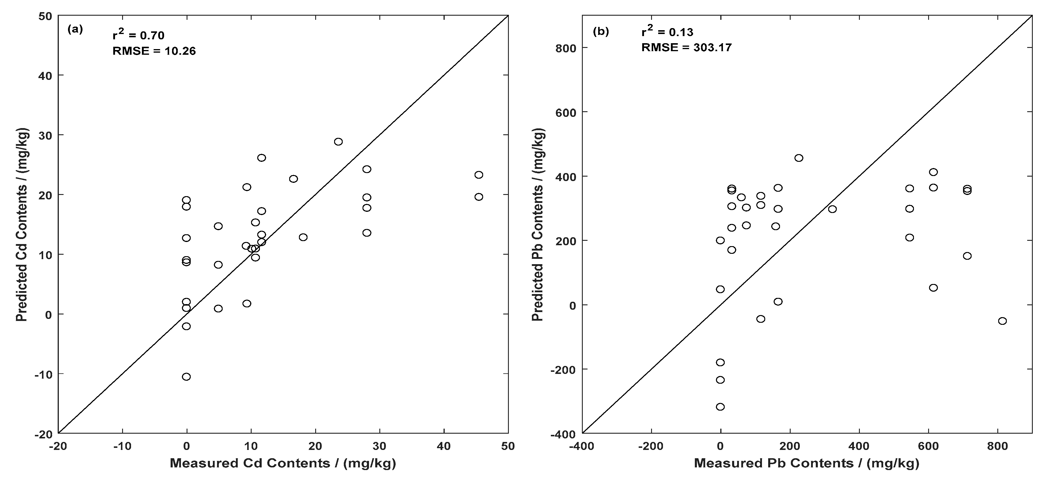
3.5. Predictions Cd and Pb Contents

Compared with SVM, PLSR performed better with higher accuracy of prediction. Therefore, in this section, results of PLSR are listed. See Section 4.2 for the comparison between the two methods.
Based on PLSR modeling and r2 evaluating, two predicted models with the highest r2 value were selected as the Cd (a) and Pb (b) contents prediction model, respectively, as shown in Figure 5.
The predictions of Cd contents reached satisfying results. The r 2 of prediction was 0.70. However, both of our PLS and SVM models failed to predict the Pb concentration accurately, with a low r 2 of 0.13 and a severely biased residual. The results indicated that it was only feasible to predict foliar Cd concentration quantitatively, and the prediction of Pb contents needs further investigation.

4. Discussion

4.1. Comparisons of Pre-Processing Methods

The pre-processing methods NorStaSG1D and SGSta1D reached greatly satisfying diagnostic accuracies. All of them were above 0.80, except for C–LCd at 0.79, as shown in Figure 6. Therefore, the abovementioned two pre-processing methods should be given the priority for diagnosing Cd–Pb cross-stress. Some significant bands, selected from the dataset after pre-processing NorStaSG1D and SGSta1D, are likely to be used as sensitive indices to quickly detect the Cd and Pb stress in leaves, which does help to apply remote sensing technology in large-scale heavy metal pollution detecting.
We have found that the combination of pre-processing methods made significant difference in diagnostic accuracies for Cd–Pb cross-stress, which coincides with Shi’s results, as shown in the reference [19]. For example, compared with the pre-processing method of NorSG, the combined method of NorSG1D showed a raised trend, no matter what types and stress levels the rice was subject to, as shown in Figure 7.
For almost all pretreatments, the corresponding diagnostic accuracies became higher with the increase of stressed levels. It is likely that the higher stressed levels of Cd–Pb cross-stress, the more obvious the change in some rice biochemical parameters (chlorophyll, water content, nitrogen content, etc.), which can be more easily detected and identified by VNIRS. These quantified stress levels can be gradually reduced to investigate the reliability of VNIRS in diagnosing low-level heavy metal pollution [13].
We also investigated the prevailing pre-processing methods of using VNIRS to estimate Cd–Pb concentrations in brief, as shown in Table 5.
The significant wavelength detected by this study for Cd stress were 681–699 nm, 738–776 nm, 880nm, 1018 nm, 1024 nm, and 1461 nm, while that for Pb were 712–728 nm, 751–784 nm, 815 nm, 1280 nm, 1476 nm, and 1601 nm. Some were closed to the previous researched results [12,13,42,56], but part of them were new conclusions, such as 880 nm and 1461 nm for Cd and 784 nm and 1601 nm for Pb. There is a closed relation between the reflectance of 670–760 nm and content of chlorophyll and nitrogen [57], some of which were same to the Cd–Pb-stressed significant bands, indicating that Cd stress and Pb stress also affected the rice photosynthesis. In addition, the Cd stresses also affected the N–H stretch, which was sensitive in the range from 1005–1015 nm [58]. These results may service the wavelength selection of hyperspectral sensors in the future.
Spectral pre-processing methods, such as SG, 1D, and average, et al. [4,12,13,56] were employed to reduce noise levels. GA and OSC are relatively less commonly used to derive stable hyperspectral signatures [12,42]. PCA is employed for spectral dimension reduction. Besides Table 5, two innovative methods, a genetic algorithm-based stacking algorithm [38] and a memory-based learning approach [39], may be worth exploring to diagnose and predict heavy metals with VNIRS datasets.

4.2. Comparisons of Estimated Models

Besides the prediction of PLSR, SVM was also conducted to estimate the Cd–Pb contents, but the latter performed not better than the former. Some evaluated parameters were showed in Table 6. Compared with SVM, PLSR predicted better with lower RMSE and RPIQ. Due to the poor performance of SVM in predicting, only PLSR was used to predict the Cd–Pb contents in rice canopy. Recently, Tsakiridis and Tziolas proposed two novel methods, namely a genetic algorithm-based stacking algorithm [38] and a memory-based learning approach [39], which presented an increase in estimated accuracies and a decrease in the RMSE about 6.47%. These innovative solutions could be considered to predict heavy metals contents and to evaluate the predictive performance in the future, especially for Pb contents prediction, which might improve the estimated accuracies and the robustness of predictive models.
To conform to the performance of predicted results, we investigated some research about estimating the Cd contents and Pb contents by VINRS in recent years. The details were displayed in Table 7.
Almost all Cd–Pb diagnosis are based on soil spectra measured in the laboratory, and the values of r2 range from 0.21 to 0.86, with great fluctuation. There is one study of the spectral monitoring part in the leaf only, without the strict conditions of the greenhouse. Although the highest value of r2 is above our article, the study includes 36 samples with a single Cd stress only. In our study, there were 96 samples, which is nearly three times the samples number in the reference [55], and our study is on Cd–Pb cross-stress with four different stressed levels. The highest r2 of Pb contents prediction was 0.73 in the above research [59], but the study involves amounts of soil sampling and wet chemical analysis. Therefore, our prediction of Cd contents was acceptable, but that of Pb stress need to be improved in the future work.

4.3. Investigations of Limits and Future Study

The study only explored the feasibility of diagnosing and predicting Cd and Pb due to limited experimental site and samples. However, there are often cross-stress of various heavy metals, such as Zn, Cu, Hg, Cr, Ni, etc. in farmland soil [11,14,41]. Therefore, it is necessary to explore possibilities of using VNIRS to diagnose and predict quantitatively the certain stress from multiple stressed types.
It is worthy to further explore modeling methods and observatory angles. In this study, we have used PLS and SVM solely to estimate the Cd–Pb concentrations in rice foliar based on the canopy reflectance. More sophisticated modeling methods, such as random forest and Lasso regression, are worthy exploring in the future studies. In addition, this study diagnosed and predicted the Cd–Pb cross-stress only from canopy hyperspectral reflectance, while other studies found that the diagnostic accuracies could be improved by combining the hyperspectral reflectance of rice plants and soil [34]. This is also interesting to verify on our target pollutant and try to use combined spectra to estimate, one step toward the reality.

5. Conclusions

In this paper, a Cd–Pb cross-stress experiment of heavy metals was designed and the feasibility of using rice canopy spectra to diagnose and predict Cd and Pb in cross-stress was explored.
It is found that the significant bands were mainly distributed in the extent of 681–776 nm and 1224–1349 nm for Cd stress and 712–784 nm for Pb stress. With the increasing concentration, the foliar reflectance generally increases for Cd stress, while it drops for Pb stress.
On one hand, all diagnostic accuracies reached 0.75 under any Cd–Pb-stressed level combination, and with the proper spectral pretreatment, the accuracy may exceed 0.85 with very few exceptions. On the other hand, the r2 was 0.70 and 0.13 for Cd and Pb contents prediction. We conclude from our limited sample size in a greenhouse condition that from the VNIRS of rice canopy it is possible to diagnose in which single or combined stress the rice crop is suffering, and it is possible to predict the foliar Cd concentration from rice canopy. However, it is worth noting that this is only one example for a trend, while a solid conclusion still needs further studies in the field and with a sufficient sample size.

Author Contributions

S.Z. writes the draft and rectifies the manuscript, and T.F. makes an investigation, rectify the manuscript, and funds the project. J.L. and Y.H. rectify the draft and make parts of visualization works. S.W. and Y.L. contribute to data measurement. Y.C. gives constructive suggestions and provides the software. All authors have read and agreed to the published version of the manuscript.

Funding

This research received no external funding.

Acknowledgments

We would like to thank Yunjiang Wang, Yinkang Wan, and Meng Bian for the help in the experiment design and programs. And thank anonymous reviewers for their helpful comments.

Conflicts of Interest

The authors declare no conflict of interest.

References

  1. Farias, C.O.; Hamacher, C.; Wagener, A.D.L.R.; Campos, R.C.D.; Godoy, J.M. Trace metal contamination in mangrove sediments, Guanabara Bay, Rio de Janeiro, Brazil. J. Braz. Chem. Soc. 2007, 18, 1194–1206. [Google Scholar] [CrossRef]
  2. Leenaers, H.; Okx, J.P.; Burrough, P.A. Employing elevation data for efficient mapping of soil pollution on floodplains. Soil Use Manag. 1990, 6, 105–114. [Google Scholar] [CrossRef]
  3. Steiger, B.V.; Webster, R.; Schulin, R.; Lehmann, R. Mapping heavy metals in polluted soil by disjunctive kriging. Environ. Pollut. 1996, 94, 205–215. [Google Scholar] [CrossRef]
  4. Liu, Y.; Li, W.; Wu, G.; Xu, X. Feasibility of estimating heavy metal contaminations in floodplain soils using laboratory-based hyperspectral data—A case study along Le’an River, China. Geo-Spat. Inf. Sci. 2011, 14, 10–16. [Google Scholar] [CrossRef] [Green Version]
  5. Rossel, R.A.V.; Walvoort, D.J.J.; Mcbratney, A.B.; Janik, L.J.; Skjemstad, J.O. Visible, near infrared, mid infrared or combined diffuse reflectance spectroscopy for simultaneous assessment of various soil properties. Geoderma 2006, 131, 59–75. [Google Scholar] [CrossRef]
  6. Allory, V.; Cambou, A.; Moulin, P.; Schwartz, C.; Cannavo, P.; Vidal-Beaudet, L.; Barthes, B.G. Quantification of soil organic carbon stock in urban soils using visible and near infrared reflectance spectroscopy (VNIRS) in situ or in laboratory conditions. Sci. Total Environ. 2019, 686, 764–773. [Google Scholar] [CrossRef] [PubMed] [Green Version]
  7. Kooistra, L.; Wehrens, R.; Leuven, R.S.; Buydens, L.M. Possibilities of visible–near-infrared spectroscopy for the assessment of soil contamination in river floodplains. Anal. Chim. Acta 2001, 446, 97–105. [Google Scholar] [CrossRef]
  8. Stenberg, B.; Rossel, R.V.; Mouazen, A.; Wetterlind, J. Visible and near infrared spectroscopy in soil science. Adv. Agron. 2010, 107, 163–215. [Google Scholar]
  9. Ren, Y.H.; Zhuang, D.F.; Singh, A.N.; Pan, J.J.; Qiu, D.S.; Shi, R.H. Estimation of As and Cu contamination in agricultural soils around a mining area by reflectance spectroscopy: A case study. Pedosphere 2009, 19, 719–726. [Google Scholar] [CrossRef]
  10. Bray, J.G.; Rossel, R.A.V.; McBratney, A.B. Diagnostic Screening of Urban Soil Contaminants Using Diffuse Reflectance Spectroscopy. Aust. J. Soil Res. 2010, 47, 43. [Google Scholar]
  11. Hong, Y.; Shen, R.; Cheng, H.; Chen, Y.; Zhang, Y.; Liu, Y.; Zhou, M.; Yu, L.; Liu, Y.; Liu, Y. Estimating lead and zinc concentrations in peri-urban agricultural soils through reflectance spectroscopy: Effects of fractional-order derivative and random forest. Sci. Total Environ. 2019, 651 Pt 2, 1969–1982. [Google Scholar] [CrossRef]
  12. Chen, T.; Chang, Q.; Clevers, J.G.; Kooistra, L. Rapid identification of soil cadmium pollution risk at regional scale based on visible and near-infrared spectroscopy. Environ. Pollut. 2015, 206, 217–226. [Google Scholar] [CrossRef] [PubMed]
  13. Wang, J.; Cui, L.; Gao, W.; Shi, T.; Chen, Y.; Gao, Y. Prediction of low heavy metal concentrations in agricultural soils using visible and near-infrared reflectance spectroscopy. Geoderma 2014, 216, 1–9. [Google Scholar] [CrossRef]
  14. Sun, W.; Skidmore, A.K.; Wang, T.; Zhang, X. Heavy metal pollution at mine sites estimated from reflectance spectroscopy following correction for skewed data. Environ. Pollut. 2019, 252 Pt B, 1117–1124. [Google Scholar] [CrossRef]
  15. Kemper, T.; Sommer, S. Estimate of heavy metal contamination in soils after a mining accident using reflectance spectroscopy. Environ. Sci. Technol. 2002, 36, 2742. [Google Scholar] [CrossRef]
  16. Wu, Z.Y.; Chen, J.; Ji, J.F.; Tian, Q.J.; Wu, X.M. Feasibility of reflectance spectroscopy for the assessment of soil mercury contamination. Environ. Sci. Technol. 2005, 39, 873–878. [Google Scholar] [CrossRef]
  17. Liu, M.; Liu, X.; Ding, W.; Wu, L. Monitoring stress levels on rice with heavy metal pollution from hyperspectral reflectance data using wavelet-fractal analysis. Int. J. Appl. Earth Obs. Geoinf. 2011, 13, 246–255. [Google Scholar] [CrossRef]
  18. Shi, T.; Chen, Y.; Liu, Y.; Wu, G. Visible and near-infrared reflectance spectroscopy-an alternative for monitoring soil contamination by heavy metals. J. Hazard Mater. 2014, 265, 166–176. [Google Scholar] [CrossRef]
  19. Shi, T.; Liu, H.; Chen, Y.; Fei, T.; Wang, J.; Wu, G. Spectroscopic Diagnosis of Arsenic Contamination in Agricultural Soils. Sensors 2017, 17, 1036. [Google Scholar] [CrossRef] [PubMed] [Green Version]
  20. Liu, M.; Liu, X.; Wu, L.; Duan, L.; Zhong, B. Wavelet-based detection of crop zinc stress assessment using hyperspectral reflectance. Comput. Geosci. 2011, 37, 1254–1263. [Google Scholar] [CrossRef]
  21. Zhang, S.; Fei, T.; Ran, Y. Diagnosis of Heavy Metal cross Contamination in Leaf of Rice Based on Hyperspectral Image: A Greenhouse Experiment. In Proceedings of the 2018 IEEE International Conference on Advanced Manufacturing (ICAM), Yunlin, China, 16 November 2018. [Google Scholar]
  22. Chakraborty, S.; Weindorf, D.C.; Deb, S.; Li, B.; Paul, S.; Choudhury, A.; Ray, D.P. Rapid assessment of regional soil arsenic pollution risk via diffuse reflectance spectroscopy. Geoderma 2017, 289, 72–81. [Google Scholar] [CrossRef]
  23. Sun, W.; Zhang, X. Estimating soil zinc concentrations using reflectance spectroscopy. Int. J. Appl. Earth Obs. Geoinf. 2017, 58, 126–133. [Google Scholar] [CrossRef]
  24. Fu, J.; Zhou, Q.; Liu, J.; Liu, W.; Wang, T.; Zhang, Q.; Jiang, G. High levels of heavy metals in rice (Oryza sativa L.) from a typical E-waste recycling area in southeast China and its potential risk to human health. Chemosphere 2008, 71, 1269–1275. [Google Scholar] [PubMed]
  25. Cheng, F.; Zhao, N.; Xu, H.; Li, Y.; Zhang, W.; Zhu, Z.; Chen, M. Cadmium and lead contamination in japonica rice grains and its variation among the different locations in southeast China. Sci. Total Environ. 2006, 359, 156–166. [Google Scholar]
  26. Keawkim, K.K.; Chuanuwatanakul, S.; Chailapakul, O.; Motomizu, S. Determination of lead and cadmium in rice samples by sequential injection/anodic stripping voltammetry using a bismuth film/crown ether/Nafion modified screen-printed carbon electrode. Food Control 2013, 31, 14–21. [Google Scholar] [CrossRef]
  27. Malley, F.D.; Williams, P.C. Use of Near-Infrared Reflectance Spectroscopy in Prediction of Heavy Metals in Freshwater Sediment by Their Association with Organic Matter. Environ. Sci. Technol. 1997, 31, 3461–3467. [Google Scholar] [CrossRef]
  28. Choe, E.; van der Meer, F.; van Ruitenbeek, F.; van der Werff, H.; de Smeth, B.; Kim, K.-W. Mapping of heavy metal pollution in stream sediments using combined geochemistry, field spectroscopy, and hyperspectral remote sensing: A case study of the Rodalquilar mining area, SE Spain. Remote Sens. Environ. 2008, 112, 3222–3233. [Google Scholar] [CrossRef]
  29. Gannouni, S.; Rebai, N.; Abdeljaoued, S. A Spectroscopic Approach to Assess Heavy Metals Contents of the Mine Waste of Jalta and Bougrine in the North of Tunisia. J. Geogr. Inf. Syst. 2012, 4, 242–253. [Google Scholar] [CrossRef] [Green Version]
  30. Vohland, M.; Bossung, C.; Fründ, H.C. A spectroscopic approach to assess trace-heavy metal contents in contaminated floodplain soils via spectrally active soil components. J. Plant Nutr. Soil Sci. 2009, 172, 201–209. [Google Scholar] [CrossRef]
  31. Wu, Y.; Chen, J.; Ji, J.; Gong, P.; Liao, Q.; Tian, Q.; Ma, H. A Mechanism Study of Reflectance Spectroscopy for Investigating Heavy Metals in Soils. Soil Sci. Soc. Am. J. 2007, 71, 918–926. [Google Scholar] [CrossRef]
  32. Wu, Y.; Zhang, X.; Liao, Q.; Ji, J. Can Contaminant Elements in Soils Be Assessed by Remote Sensing Technology: A Case Study With Simulated Data. Soil Sci. 2011, 176, 196–205. [Google Scholar] [CrossRef]
  33. Wu, Y.; Chen, J.; Wu, X.; Tian, Q.; Ji, J.; Qin, Z. Possibilities of reflectance spectroscopy for the assessment of contaminant elements in suburban soils. Appl. Geochem. 2005, 20, 1051–1059. [Google Scholar] [CrossRef]
  34. Shi, T.; Wang, J.; Chen, Y.; Wu, G. Improving the prediction of arsenic contents in agricultural soils by combining the reflectance spectroscopy of soils and rice plants. Int. J. Appl. Earth Obs. Geoinf. 2016, 52, 95–103. [Google Scholar] [CrossRef]
  35. Liu, M.; Liu, X.; Li, J.; Li, T. Estimating regional heavy metal concentrations in rice by scaling up a field-scale heavy metal assessment model. Int. J. Appl. Earth Obs. Geoinf. 2012, 19, 12–23. [Google Scholar] [CrossRef]
  36. Chang, C.; Laird, D.A.; Mausbach, M.J.; Hurburgh, C.R. Near-Infrared Reflectance Spectroscopy–Principal Components Regression Analyses of Soil Properties. Soil Sci. Soc. Am. J. 2001, 65, 480–490. [Google Scholar] [CrossRef] [Green Version]
  37. Mouazen, M.A.; Kuang, B.; Baerdemaeker, J.D.; Ramon, H.; Guerrero, C.; Rossel, R.A.V.; Mouazen, A.M. Comparison among principal component, partial least squares and back propagation neural network analyses for accuracy of measurement of selected soil properties with visible and near infrared spectroscopy. Geoderma 2010, 158, 23–31. [Google Scholar] [CrossRef]
  38. Tsakiridis, L.N.; Tziolas, N.V.; Theocharis, J.B.; Zalidis, G.C. A genetic algorithm-based stacking algorithm for predicting soil organic matter from vis–NIR spectral data. Eur. J. Soil Sci. 2019, 70, 578–590. [Google Scholar] [CrossRef]
  39. Tziolas, N.; Tsakiridis, N.; Ben-Dor, E.; Theocharis, J.; Zalidis, G. A memory-based learning approach utilizing combined spectral sources and geographical proximity for improved VIS-NIR-SWIR soil properties estimation. Geoderma 2019, 340, 11–24. [Google Scholar] [CrossRef]
  40. Mitchell, J.J.; Glenn, N.F.; Sankey, T.T.; Derryberry, D.R.; Germino, M.J. Remote sensing of sagebrush canopy nitrogen. Remote Sens. Environ. 2012, 124, 217–223. [Google Scholar] [CrossRef] [Green Version]
  41. Liu, J.; Han, J.; Xie, J.; Wang, H.; Tong, W.; Ba, Y. Assessing heavy metal concentrations in earth-cumulic-orthic-anthrosols soils using Vis-NIR spectroscopy transform coupled with chemometrics. Spectrochim. Acta A Mol. Biomol. Spectrosc. 2020, 226, 117639. [Google Scholar] [CrossRef]
  42. Jiang, Q.; Liu, M.; Wang, J.; Liu, F. Feasibility of using visible and near-infrared reflectance spectroscopy to monitor heavy metal contaminants in urban lake sediment. Catena 2018, 162, 72–79. [Google Scholar] [CrossRef]
  43. Qian, Y.; Chen, C.; Zhang, Q.; Li, Y.; Chen, Z.; Li, M. Concentrations of cadmium, lead, mercury and arsenic in Chinese market milled rice and associated population health risk. Food Control 2010, 21, 1757–1763. [Google Scholar] [CrossRef]
  44. Xie, H.L.; Tang, S.Q.; Wei, X.J.; Shao, G.N.; Jiao, G.A.; Sheng, Z.H.; Luo, J.; Hu, P.S. The cadmium and lead content of the grain produced by leading Chinese rice cultivars. Food Chem. 2017, 217, 217–224. [Google Scholar] [CrossRef] [PubMed]
  45. MEE; SAMR. Risk Control Standard for Soil Contamination of Agricultural Land 2018; Standards Press of China: Beijing, China, 2018; pp. 1–7. [Google Scholar]
  46. Shi, T.; Liu, H.; Chen, Y.; Wang, J.; Wu, G. Estimation of arsenic in agricultural soils using hyperspectral vegetation indices of rice. J. Hazard. Mater. 2016, 308, 243–252. [Google Scholar] [CrossRef]
  47. Savitzky, A.; Golay, M.J.E. Smoothing and Differentiation of Data by Simplified Least Squares Procedures. Anal. Chem. 1964, 36, 1627–1639. [Google Scholar] [CrossRef]
  48. Kampichler, C.; Wieland, R.; Calmé, S.; Weissenberger, H.; Arriaga-Weiss, S. Classification in conservation biology: A comparison of five machine-learning methods. Ecol. Inform. 2010, 5, 441–450. [Google Scholar] [CrossRef]
  49. Haaland, M.D.; Thomas, E.V. Partial least-squares methods for spectral analyses. 1. Relation to other quantitative calibration methods and the extraction of qualitative information. Anal. Chem. 1988, 60, 1193–1202. [Google Scholar] [CrossRef]
  50. Darvishzadeh, R.; Skidmore, A.; Schlerf, M.; Atzberger, C.; Corsi, F.; Cho, M. LAI and chlorophyll estimation for a heterogeneous grassland using hyperspectral measurements. Isprs J. Photogramm. Remote Sens. 2008, 63, 409–426. [Google Scholar] [CrossRef]
  51. Schlerf, M.; Atzberger, C.; Hill, J. Remote sensing of forest biophysical variables using HyMap imaging spectrometer data. Remote Sens. Environ. 2005, 95, 177–194. [Google Scholar] [CrossRef] [Green Version]
  52. Bellon-Maurel, V.; Fernandez-Ahumada, E.; Palagos, B.; Roger, J.-M.; McBratney, A. Critical review of chemometric indicators commonly used for assessing the quality of the prediction of soil attributes by NIR spectroscopy. TrAC Trends Anal. Chem. 2010, 29, 1073–1081. [Google Scholar] [CrossRef]
  53. He, L.; Zhang, H.Y.; Zhang, Y.S.; Song, X.; Feng, W.; Kang, G.Z.; Wang, C.Y.; Guo, T.C. Estimating canopy leaf nitrogen concentration in winter wheat based on multi-angular hyperspectral remote sensing. Eur. J. Agron. 2016, 73, 170–185. [Google Scholar] [CrossRef]
  54. Kooistra, L.; Salas, E.A.L.; Clevers, J.G.P.W.; Wehrens, R.; Leuven, R.S.E.W.; Nienhuis, P.H.; Buydens, L.M.C. Exploring field vegetation reflectance as an indicator of soil contamination in river floodplains. Environ. Pollut. 2004, 127, 281–290. [Google Scholar] [CrossRef]
  55. Wang, T.; Wei, H.; Zhou, C.; Gu, Y.; Li, R.; Chen, H.; Ma, W. Estimating cadmium concentration in the edible part of Capsicum annuum using hyperspectral models. Environ. Monit. Assess. 2017, 189, 548. [Google Scholar] [CrossRef]
  56. Cheng, H.; Shen, R.; Chen, Y.; Wan, Q.; Shi, T.; Wang, J.; Wan, Y.; Hong, Y.; Li, X. Estimating heavy metal concentrations in suburban soils with reflectance spectroscopy. Geoderma 2019, 336, 59–67. [Google Scholar] [CrossRef]
  57. Mutanga, O.; Skidmore, A.K. Hyperspectral band depth analysis for a better estimation of grass biomass (Cenchrus ciliaris) measured under controlled laboratory conditions. Int. J. Appl. Earth Obs. Geoinf. 2004, 5, 87–96. [Google Scholar] [CrossRef]
  58. Curran, P. Remote sensing of foliar chemistry. Remote Sens. Environ. 1990, 30, 271–278. [Google Scholar] [CrossRef]
  59. Kemper, T.; Ehlers, M.; Sommer, S.; Posa, F.; Kaufmann, H.J.; Michel, U.; de Carolis, G. Use of airborne hyperspectral data to estimate residual heavy metal contamination and acidification potential in the Guadiamar floodplain Andalusia, Spain after the Aznacollar mining accident. In Proceedings of the Remote Sensing for Environmental Monitoring, GIS Applications, and Geology IV, International Society for Optics and Photonics, Canary Islands, Spain, 22 October 2004; Volume 5574, pp. 224–234. [Google Scholar]
Figure 1. Cadmium-Lead (Cd–Pb) concentrations, the corresponding abbreviations and combined details.
Remotesensing 12 00469 g001
Figure 2. Workflow of the Experiment.
Remotesensing 12 00469 g002
Figure 3. Numbers of significant bands selected with different pre-processing methods.
Remotesensing 12 00469 g003
Figure 4. Ranges of spectral response for Cd-stressed (a,c) and Pb-stressed (b,d).
Remotesensing 12 00469 g004
Figure 5. Predictions of Cd contents (a) and predictions of Pb contents (b) in cross-stress based on partial least squares regression (PLSR).
Remotesensing 12 00469 g005
Figure 6. Diagnostic accuracies of different types and stress levels with NorStaSG1D (Left) and SGSta1D (Right). (NorStaSG1D is a pre-processing method with normalization, standardization, Savitzky-Golay smoothing, and 1st-Derivative, successively, while SGSta1D is a pre-processing method with Savitzky-Golay smoothing, standardization, and 1st-Derivative, successively).
Remotesensing 12 00469 g006
Figure 7. Diagnostic accuracies of Cd stress (a) and Pb stress (b) based on NorSG and NorSG1D. (NorSG is a pre-processing method with normalization and Savitzky-Golay smoothing, successively, while NorSG1D is a pre-processing method with normalization, Savitzky-Golay smoothing, and 1st-Derivative, successively).
Remotesensing 12 00469 g007
Table 1. Pre-processing methods and their corresponding abbreviations.
Pre-processing MethodsAbbreviations
Normalization + Savitzky–Golay smoothing + 1st-DerivativeNorSG1D
Savitzky–Golay smoothing + normalization + 1st-DerivativeSGNor1D
Savitzky–Golay smoothing + normalization + 2nd-DerivativeSGNor2D
Savitzky–Golay smoothing + standardization + 1st-DerivativeSGSta1D
Savitzky–Golay smoothing + standardization + 2nd-DerivativeSGSta2D
Normalization + standardization + Savitzky–Golay smoothing + 1st-DerivativeNorStaSG1D
Normalization + standardization + Savitzky–Golay smoothing + 2nd-DerivativeNorStaSG1D
Normalization + Savitzky–Golay smoothing + standardization + 1st-DerivativeNorSGSta1D
Normalization + Savitzky–Golay smoothing + standardization + 2nd-DerivativeNorSGSta2D
Standardization + Savitzky–Golay smoothing + normalization + 1st-DerivativeStaSGNor1D
Table 2. Statistical Description of the leaf Cadmium-Lead (Cd–Pb) Contents (mg kg−1) for the whole data sets, calibration datasets, and validation data sets.
Cd Contents MeasuredPb Contents Measured
Whole Data SetCalibration Data SetValidation Data SetWhole Data SetCalibration Data SetValidation Data Set
num966432966432
maximum45.4845.4845.48814.91814.91814.91
minimum000000
mean12.9613.2912.31240.87230.36261.88
SD11.9311.6612.62270.23269.04275.69
Table 3. Diagnostic details of C–ZPb with NorStaSG1D pre-processing (C-ZPb is zero Pb concentration of cross stress, and NorStaSG1D is a pre-processing method with normalization, standardization, Savitzky-Golay smoothing, and 1st-Derivative, successively).
Sample NumberCorrect DiagnosisIncorrect Diagnosis Accuracy
C–ZPb24 21 3 0.88
Other Stress Levels726480.89
Statistical data9685110.89
Table 4. Diagnostic accuracies for Cd–Pb cross-stress with different pretreatment methods.
Pretreatment methodsDiagnostic accuracies of CdDiagnostic accuracies of Pb
C–ZCdC–LCdC–MCdC–HCdC–ZPbC–LPbC–MPbC–HPd
NorSG1D0.86 0.75 0.81 0.83 0.86 0.81 0.83 0.92
NorStaSG1D0.86 0.79 0.85 0.90 0.89 0.85 0.85 0.88
NorStaSG2D0.81 0.77 0.81 0.81 0.85 0.81 0.85 0.88
NorSGSta1D0.85 0.75 0.88 0.88 0.91 0.90 0.88 0.90
NorSGSta2D0.81 0.75 0.83 0.81 0.88 0.81 0.88 0.88
StaSGNor1D0.82 0.75 0.83 0.85 0.86 0.85 0.85 0.88
SGNor1D0.86 0.77 0.90 0.90 0.86 0.85 0.85 0.88
SGNor2D0.83 0.81 0.83 0.83 0.86 0.83 0.79 0.85
SGSta1D0.86 0.79 0.85 0.90 0.91 0.90 0.88 0.90
SGSta2D0.81 0.75 0.79 0.81 0.88 0.85 0.85 0.88
Table 5. Methods of hyperspectral data pre-processing for estimating Cd–Pb concentrations.
CategoriesPre-Processing MethodsImportant Bands (\nm)Refs
Cdprincipal component analysis (PCA)700–710[54]
CdFirst derivative(1D)372, 374, 478[55]
Cdorthogonal signal correction (OSC), ABS,
1D, second derivative(2D), et al.
590–620, 580–595[12]
Cdgenetic algorithm (GA)481, 563, 616, 718[42]
CdSavitzky–Golay smoothing (SG)2100–2300[56]
Cd1D,2D, normalization, standardization681, 683, 693, 694, 699, 769–776, 880, 1018, 1461, etc.This work
PbPCA700–710[54]
PbGA617, 735, 2350 [42]
PbSG710–720, 2100–2300[56]
Pbaverage564, 624[4]
Pbabsorbance transformation (ABS), SG400–450, 1000, 2400–2420[13]
PbFractional order derivative (FOD) 400–560[11]
Pb1D,2D, normalization, standardization712–713, 717–720, 727–728, 751–752, 757–758, 815, etc.This work
Table 6. Evaluated parameters of support vector machine (SVM) prediction and partial least squares regression (PLSR) predication.
ModelsFactor Numbersr2RMSERPIQ
CdPbCdPbCdPbCdPb
SVM430.380.2950.45421.569.7215.79
PLSR220.700.1310.26303.171.937.37
Table 7. Predicted accuracies of using visible and near-infrared reflectance spectroscopy (VNIRS) based on PLSR for recent research.
Monitoring ObjectSampling SiteMeasuring SiteMonitoring PartSample Numberr2Reference
CdRiver floodplainslabsoil360.21[54]
CdIrrigation regionlabsoil76<0.72[12]
Cd-fieldleaf360.86[55]
CdLake sedimentlabsoil1030.47[42]
CdSuburbanlabsoil930.76[56]
PbMining areaslabsoil2140.73[59]
PbRiver floodplainslabsoil360.21[54]
PbMining areaslabsoil300.59[4]
PbPaddy fieldlabsoil140.46[13]
PbLake sedimentlabsoil1030.41[42]
PbSuburbanlabsoil930.27[56]

