Characteristics Analysis and Fuzzy Fractional-Order PID Parameter Optimization for Primary Frequency Modulation of a Pumped Storage Unit Based on a Multi-Objective Gravitational Search Algorithm

Abstract

Compared with conventional hydropower units, the pumped storage unit has the characteristics of diverse working conditions and frequent switching. Therefore, the stability and regulation quality of the primary frequency modulation transition process of the regulating system is very important. Due to the “S” characteristics of the pumped storage unit (PSU), the pumped storage unit regulating system has a strong nonlinearity, and the conventional proportional-integral-derivative (PID) controller cannot provide high-quality control under low water head conditions. In this paper, the nonlinear PSU model with an elastic water hammer effect is studied, and the fuzzy fractional-order PID (FFOPID) controller is designed to improve the stability of the system. The membership function and the control parameters of the fractional-order PID are optimized based on the multi-objective gravitational search algorithm (MOGSA). The experimental results show that the optimized design of the FFOPID controller has better control quality than the traditional PID controller, the fractional-order PID (FOPID) controller, and the fuzzy PID controller (FPID) when the system is disturbed by the rotating speed under low water head.

1. Introduction

With the constant cost of traditional energy sources and the increasing pollution of the environment, the use of renewable energy has received extensive attention. Due to the simple adjustment process, fast adjustment speed, and economy of the pumped storage unit (PSU), it mainly undertakes the task of peaking and frequency modulation in the power system [1,2]. In recent years, with the formation of regional power grids, equipment fault diagnosis and the primary frequency modulation of the pumped storage unit regulating system has played a vital role in the safe and stable operation of the power system [3,4,5,6]. In previous primary frequency modulation studies, the modeling of PSU usually adopts the simplified linear model and the water diversion system model is based on the rigid water hammer theory [7,8]. However, the model of PSU is a complex nonlinear system [9]. In addition, the impact of elastic water hammer on pipeline must be considered for the pumped storage unit regulating system with a long water diversion system [10]. Therefore, it is necessary to establish a nonlinear pumped storage unit regulating system model to obtain the transient characteristic curves under primary frequency modulation.

Moreover, when the pumped storage unit regulating system performs a frequency modulation under low water head conditions, the unit speed of PSU will be relatively large, and it is easy to enter the anti-pump area in the “S” area, which will lead to low-frequency oscillation [11,12,13]. As pumped storage units play an increasingly important role in grid frequency modulation, it is essential to propose a new type of controller to replace the traditional proportional-integral-derivative (PID) controller. Hence, this paper proposes a fuzzy fractional-order PID (FFOPID) controller for the pumped storage unit regulating system. Compared with the traditional integer-order PID controller, the fractional-order PID (FOPID) controller, the fuzzy logic control has proven to be a successful control method for many complex nonlinear systems, and even non-analytical systems [14,15,16,17,18]. In [14], Li et al. designed a fuzzy PID controller for a nonlinear hydraulic turbine governing system. In [15], Mohanty et al. presented a comprehensive analytical study of a fuzzy proportional–integral–derivative controller with a derivative filter for automatic generation control in the multi-area power system. In [16], Sahu et al. proposed a fuzzy PID controller for power systems based on the LUS–TLBO algorithm. In [17], Xu et al. studied an adaptive controller based on fuzzy theory for the pumped storage unit. In [18], Wang et al. represented a linear CARMA model for nonlinear systems with the help of the Takagi–Sugeno fuzzy linearization theory. Furthermore, in many cases, the FFOPID controller has been proposed as an alternative to traditional control techniques. Zamani et al. proposed the use of an FFOPID controller in a smart vibration isolation structure [19]. Arya et al. designed an FFOPID controller for automatic generation control of multi-zone multi-source power generation systems [20]. The above researches have proven that the FFOPID controller shows better performance and robustness.

In the process of primary frequency modulation, two factors are mainly considered. The first is the settling time of the rotational speed of the PSU, which reflects the stability time of the grid frequency. The other is the change law of the vane, which affects the water fluctuation in the pressure pipeline [21,22]. To obtain a comprehensive index between the guide vane opening and frequency variation, the multi-objective gravitational search algorithm (MOGSA) was adopted [23,24,25,26]. The gravitational search algorithm (GSA) is a random search algorithm based on the law of interaction between gravity and mass [27,28]. Standard GSA, standard MOGSA, and some improved GSA algorithms are widely used in the field of new energy, such as parameter optimization and identification of nuclear [29], wind [30], and hydropower generating unit regulation systems [8,31]. Based on the above, MOGSA is selected as the joint optimization membership function and parameter optimization tool of the fuzzy controller in this paper.

The main contribution of this paper is the design and optimization of an FFOPID controller for the nonlinear pumped storage unit regulating system with elastic water hammer effect under the condition of primary frequency modulation. Firstly, an FFOPID controller based on the fuzzy theory is designed for the nonlinear PSU model. Secondly, a multi-objective method is adopted to optimize the speed regulation time of PSU and the change law of guide vane at primary frequency modulation.

The rest of this paper is organized as follows: Section 2 gives the models of the pumped storage unit regulating system nonlinear model and the design of the FFOPID controller. In Section 3, the MOGSA algorithm is presented and verified. Section 4 gives the experimental results. Section 5 presents the conclusion.

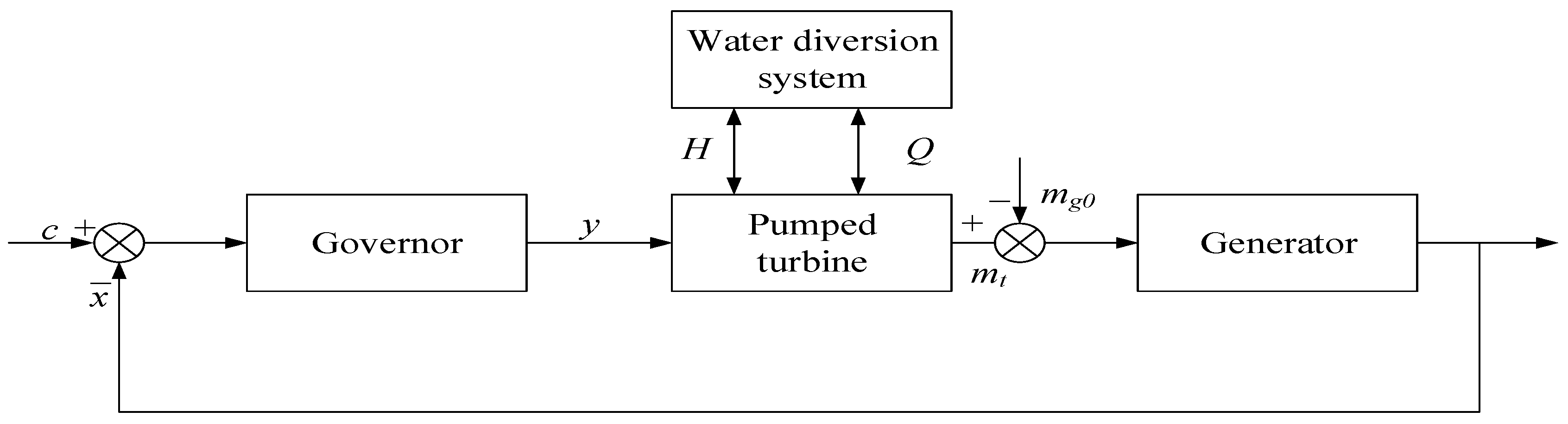
2. Model of the Pumped Storage Unit Regulating System

The pumped storage unit regulating system is a feedback control system composed of a water diversion system, governor (including servo mechanism and controller), pumped storage unit, generator, and load units. In this section, the mathematical model of a single pipe and a single turbine is established. Figure 1 is the structure of a pumped storage unit regulating system.

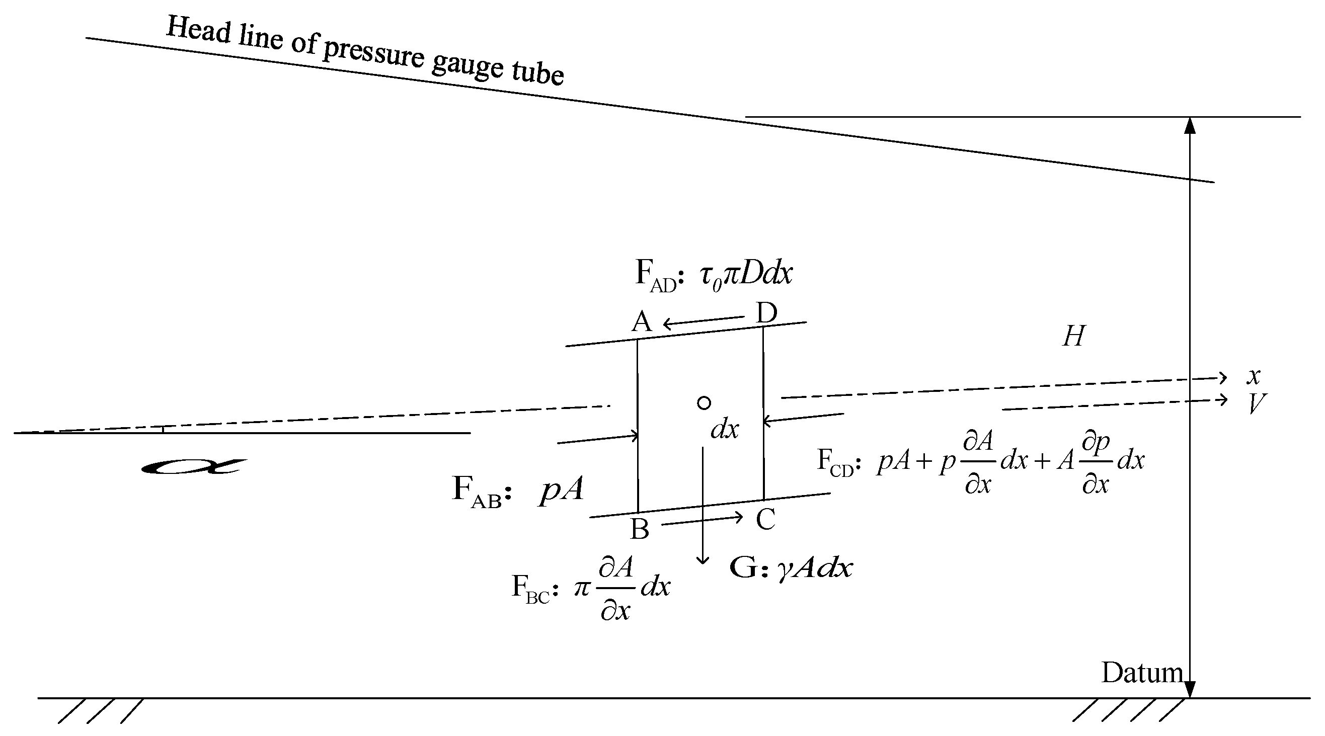
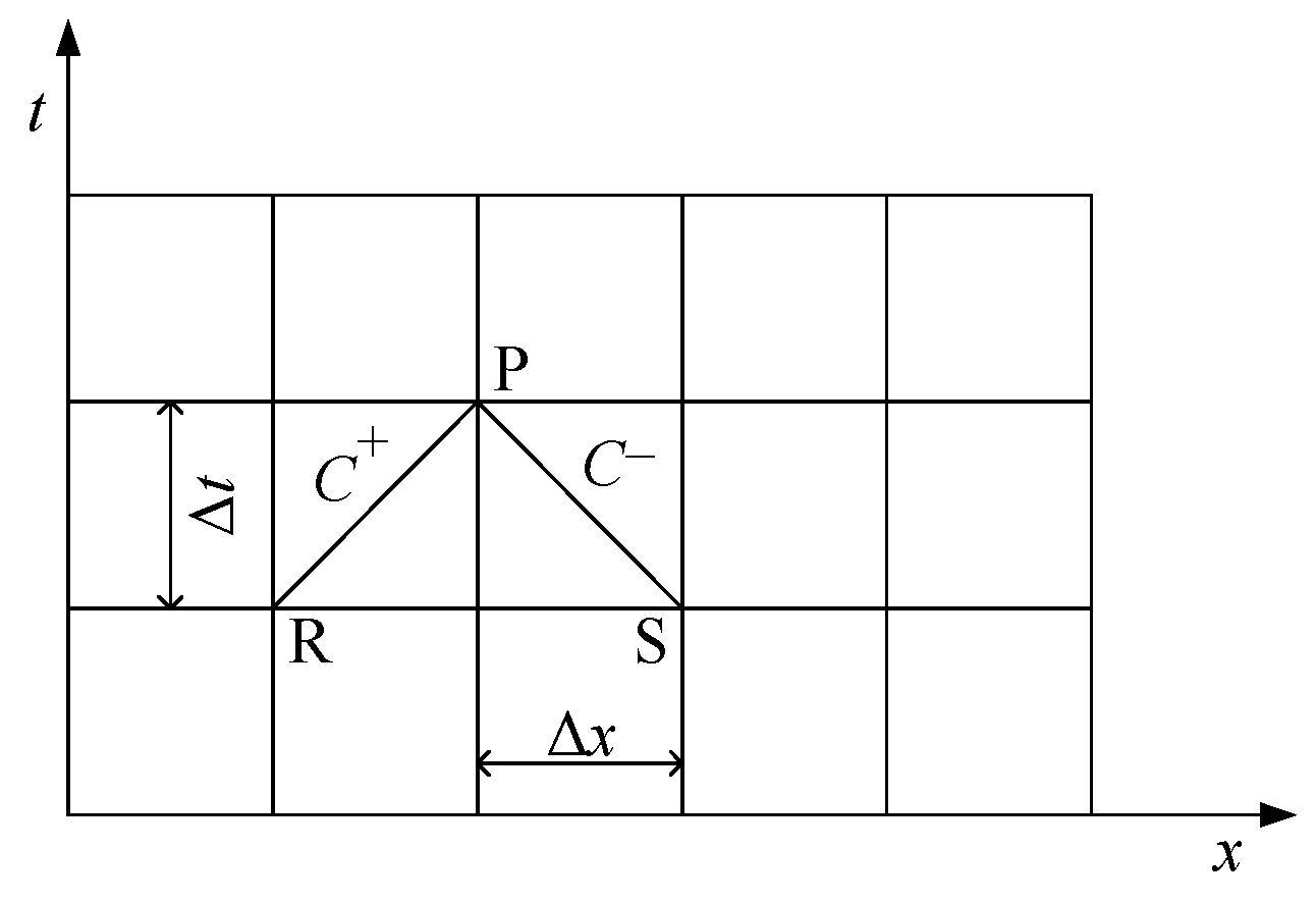
2.1. The Model of the Water Diversion System

The elastic water hammer in the pressure pipeline considers the compressibility of water and the elasticity of the pipe. The basic equation of the water hammer consists of two equations: The motion equation and the continuous equation in the water hammer process [32,33]. The basic equation of the water hammer is the mathematical expression of the law of constant flow with pressure, which reflects the change law of flow velocity and water head in the hydraulic transition process. The differential segment with length $dx$ taken out of the pipeline system is shown in Figure 2.

The differential segment dx is subject to the friction force $F_{AD}$ against the fluid from the pipe wall on surface $AD$, the pressure $F_{AB}$ on surface $AB$, the pressure $F_{BC}$ on the fluid from the pipe wall on surface $BC$, the pressure $F_{CD}$ on surface $CD$, and the gravity $G$. Before deriving Equation (1), the following assumptions must be made: The flow in the pipeline system is one-dimensional flow; the flow in each section of the pipeline system is assumed to be gradual flow; the resistance loss formula for calculating the constant flow in the pipeline can also be used to calculate the unsteady flow. According to Newton’s second law, the force equation of the differential segment dx is as follows:

$$A\frac{\partial \mathrm{p}}{\partial x}+{\tau }_0\pi D+\gamma A\sin \alpha +\mathsf{\rho }A\frac{dV}{dt}=0$$

(1)

where $P$ is the pressure at the center of the $AB$ section; $A$ is the flow area of the pipeline; ${\tau }_0$ is the shear stress of the pipe wall acting on the fluid periphery; $D$ is pipe diameter; $\gamma$ is the fluid bulk density; $\alpha$ is the angle between the pipe centerline and the horizontal line; and $V$ is the average velocity.

Since the shear stress ${\tau }_0$ of a non-constant flow is a very complicated and unresolved problem, we have to borrow the research results of the constant flow to approximate the shear stress in the unsteady flow. The shear stress direction is always opposite to the flow velocity. In the actual work, we use the water head $H$ as the main parameter, so we change $P$ to $H$. In the water diversion system of a hydropower station, the rate of change of the flow rate $Q$ with space is small, so it is neglected. Moreover, the rate of change of the density $p$ and the flow area of the pipeline $A$ along $x$ is much smaller than the rate of change of the flow rate $V$, so it is ignored. According to Equation (1), the basic equations describing water hammer can be obtained as the motion equation and the continuous equation:

$${gA}^2\frac{\partial H}{\partial x}+Q\frac{\partial Q}{\partial x}+A\frac{\partial Q}{\partial \mathrm{t}}+\frac{fQ\left|Q\right|}{2D}=0$$

(2)

$$\frac{\partial H}{\partial \mathrm{t}}+V\frac{\partial H}{\partial x}+Vsin\alpha +\frac{a^2}{g}\frac{\partial V}{\partial x}=0$$

(3)

where $Q$ is the flow rate of a certain section at time $t$; $\left|Q\right|$ is the absolute value of the flow, which is positive or negative depending on the direction of the flow; $H$ is the water head at time $t$ of the section at a corresponding datum; $\mathrm{g}$ is the acceleration of gravity; $\mathrm{a}$ is the propagation velocity of water hammer wave; and $f$ is the pipeline friction coefficient.

By integrating Equations (2) and (3) along the characteristic line $C^{+}$ and $C^{-}$, as shown in Figure 3, it can be converted into the following characteristic equation [33]:

$$C^{+}:Q_P=C_p-C_a{H}_p$$

(4)

$$C^{-}:Q_P=C_n+C_a{H}_p$$

(5)

where $C_P=Q_R+C_a{H}_R-R{Q}_R\left|Q_R\right|$, $C_n=Q_S-C_a{H}_S-R{Q}_S\left|Q_S\right|$, $C_a=\frac{gA}{a}$, $R=\frac{f\Delta t}{2DA}$. The $C_a$ and $R$ are constants; $\Delta t$ for time step, it is necessary to meet the Courant stability condition $\Delta t <\frac{\Delta x}{(a+V)}$. For the internal nodes of the pipeline, the value of flow $Q_P$ can be solved:

$$Q_P=\frac{\left(C_P{+C}_n\right)}{2}$$

(6)

The value of $H_P$ can be obtained by Equation (4) or Equation (5). In this way, the pressure and flow rate of each node in the pipeline can be obtained at all times.

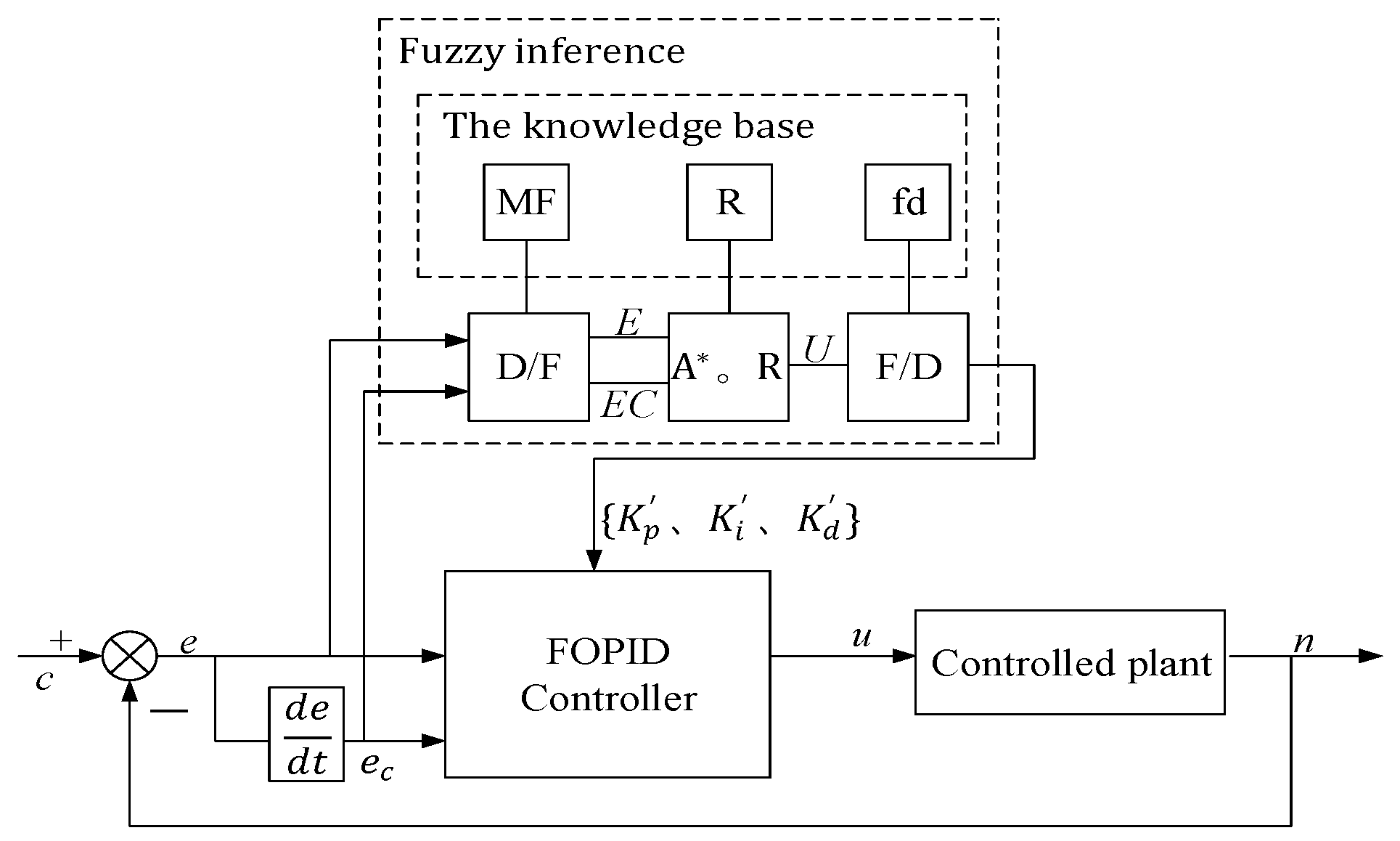
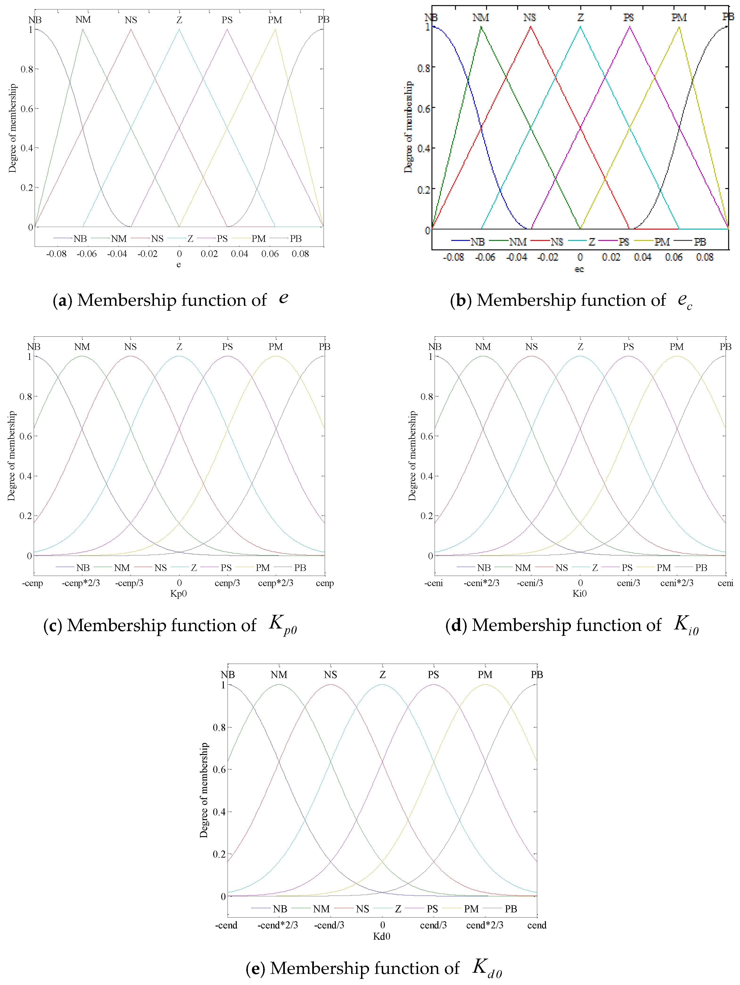
2.2. The Model of Fuzzy Fractional-Order PID Controller

2.2.1. FOPID Controller

The transfer function of conventional integer solution PID controller can be described as:

$$\mathrm{G}(s)=\frac{U(s)}{E(s)}=K_p+\frac{K_i}{s}+K_{d}s$$

(7)

where $U(s)$ is the output of the controller, and E(s) is the error input of the controller. The traditional integer-order PID controller adjusts the system performance by $K_p$, $K_i$, and $K_d$. The fractional-order $P{I}^{\mathsf{\lambda }}{D}^{\mathsf{\mu }}$ controller has the same three parameters as the PID controller: $K_p$, $K_i$, and $K_d$. Two new parameters are added: Integral order $\mathsf{\lambda }$ and differential order $\mathsf{\mu }$. The conventional PID controller is just fixed value on the coordinate axis, while the fractional order $P{I}^{\mathsf{\lambda }}{D}^{\mathsf{\mu }}$ controller is fixed value on the entire coordinate plane.

The transfer function of FOPID controller can be described as [34]:

$$\mathrm{G}(s)=\frac{U(s)}{E(s)}=K_p+\frac{K_i}{s^{\mathsf{\lambda }}}+K_d{s}^{\mathsf{\mu }}$$

(8)

Depending on the order of the control object, the $\mathsf{\lambda }$ and $\mathsf{\mu }$ ranges are adjusted. $\mathsf{\lambda }$ mainly affects the steady-state accuracy of the system, while $\mathsf{\mu }$ mainly affects the overshoot of the system. With the addition of two degrees of freedom, the FOPID controller is more flexible and has a wider range of control. The most common method to realize fractional-order transfer functions in simulation or practical research is to approach them by integer-order transfer functions [31]. In [35], Oustaloup proposed an approximate method using the recursive distribution of N poles and N zeros. To achieve a balance between the complexity and accuracy of the FFOPID controller, a 5th order Oustaloup’s recursive approximation is performed for the integral-differential operator in the selected frequency band of $\omega \in \left\{{10}^{-2},{10}^2\right\}$ rad/s. The high-order filter is as follows:

$${\mathrm{G}}_f(s)=s^{\alpha }=K{\displaystyle \prod _{k=-N}^N\frac{s+{\omega }_k^{\prime }}{s+{\omega }_k}}$$

(9)

where the poles ${\omega }_k^{\prime }$, zeros ${\omega }_k$, and gain $K$ of the filter are obtained from the following formula:

$${\omega }_k^{\prime }={\omega }_b{\left(\frac{{\omega }_h}{{\omega }_b}\right)}^{\frac{k+N+\frac{1}{2}(1-\alpha )}{2N+1}},{\omega }_k={\omega }_b{\left(\frac{{\omega }_h}{{\omega }_b}\right)}^{\frac{k+N+\frac{1}{2}(1+\alpha )}{2N+1}},K={\omega }_h^{\alpha }$$

(10)

where $\alpha$ is the order of differ-integration and $\alpha \in (0,1)$, $(2N+1)$ is the order of filter. The Laplace transform $\alpha$-th derivative with $\alpha \in R^{+}$ of a signal $x(t)$ relaxed at $t=0$ is as follows:

$$\mathrm{L}\left\{{}_{a}D_{\alpha }^{t}x(t)\right\}=s^{\alpha }X(s)$$

(11)

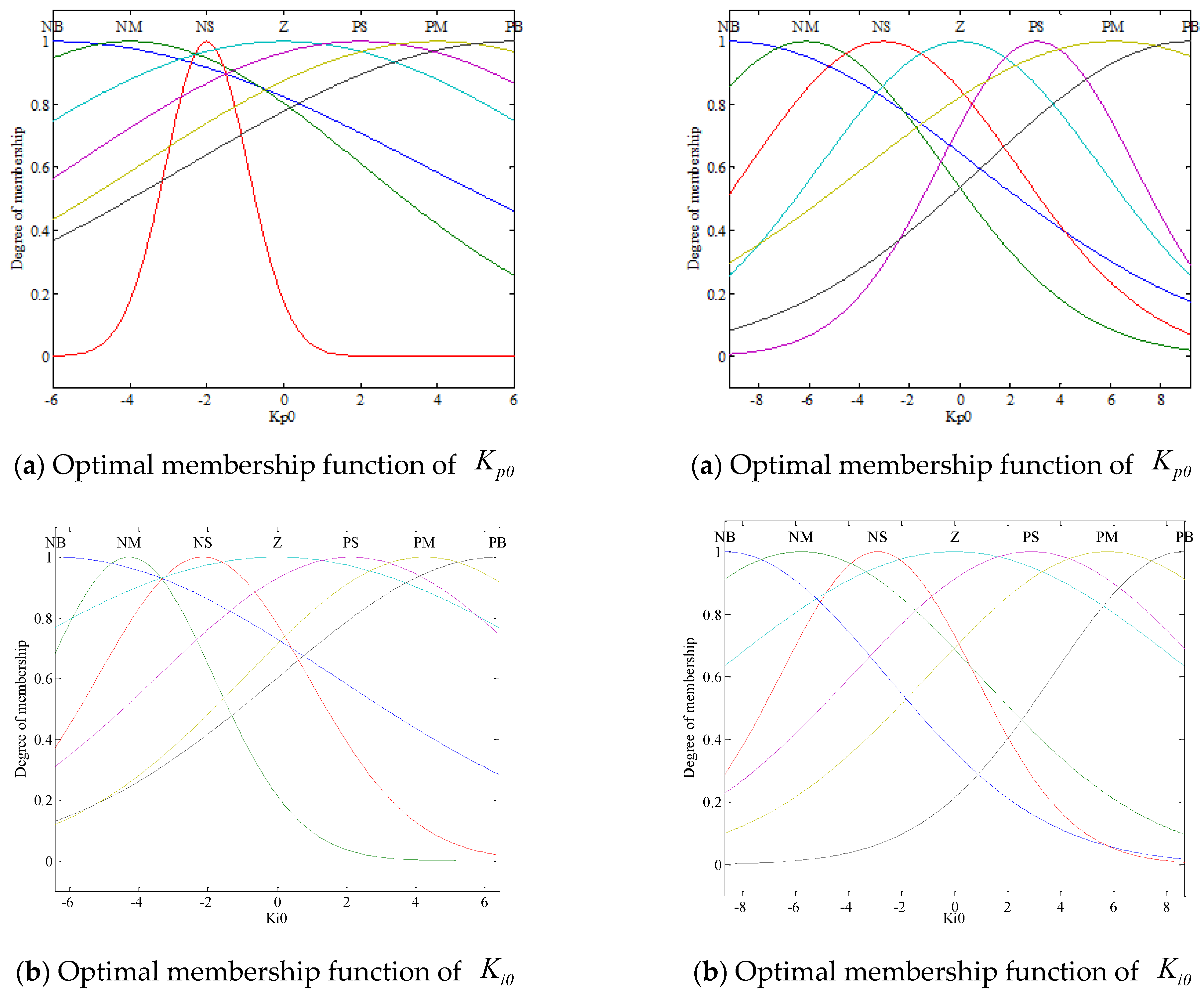
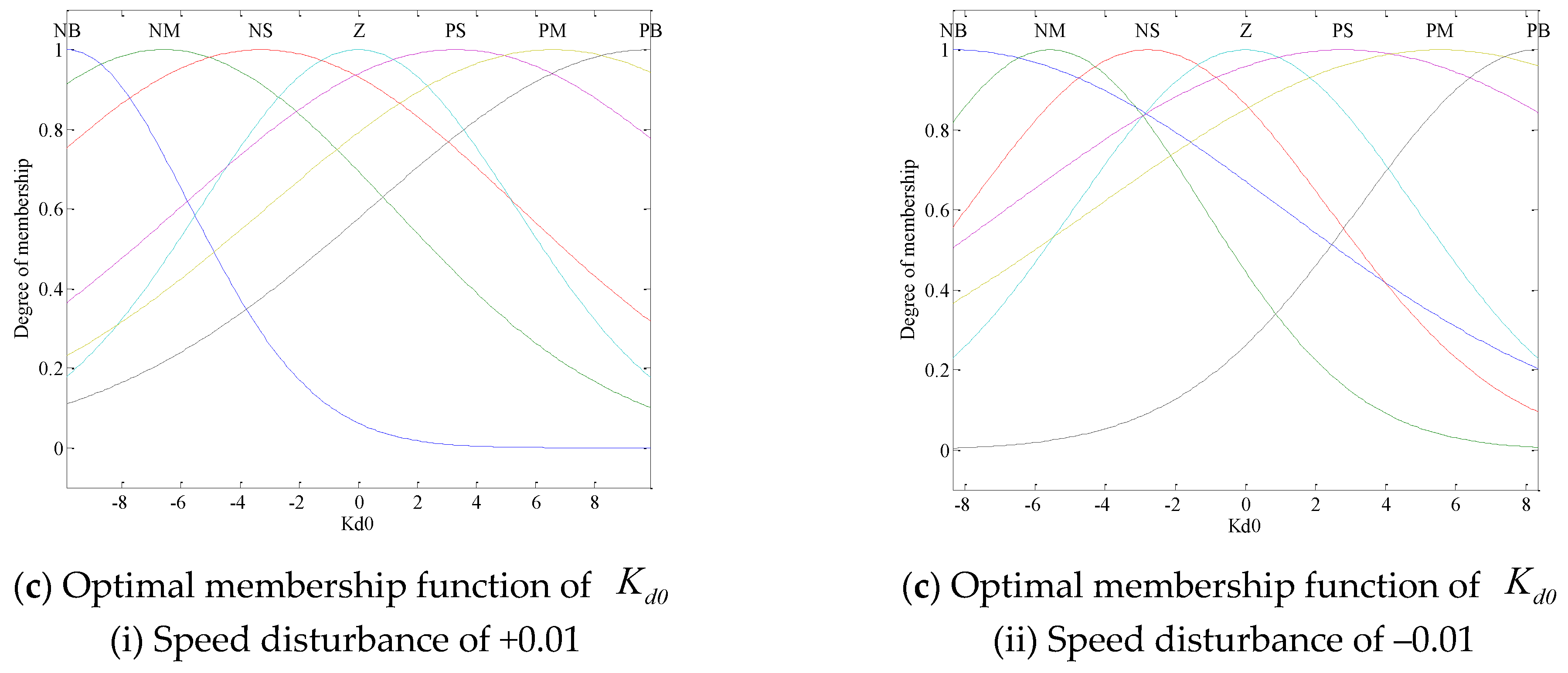
2.2.2. FFOPID Controller

Based on fuzzy set theory and fuzzy reasoning, fuzzy control transforms the knowledge and control experience expressed by expert language into fuzzy rules, which are controlled by computer. When the rotational speed of PSU deviates from the rated value, the FFOPID controller in the system operation process continuously calculates $e$ (deviation) and $e_c$ (rate of deviation change), according to the fuzzy rule principle online adjustment $\left\{K_p,K_i,K_d\right\}$, so that the system can reach a stable state. The basic structure of FFOPID controller is shown in Figure 4.

The modules $\mathrm{MF}$, $\mathrm{R}$, and $\mathrm{fd}$ in the “knowledge base” in Figure 4 are, respectively, the membership function, the fuzzy rule, and the sharpening algorithm, which are obtained offline. The core modules of the fuzzy controller: Fuzzy module ($\mathrm{D}/\mathrm{F}$), approximate reasoning module (${\mathrm{A}}^{*}{}_{\mathrm{o}}\mathrm{R}$), and sharpening module ($\mathrm{F}/\mathrm{D}$). The D/F module completes the operation of converting the clear quantity into the fuzzy quantity. In this experiment, the fuzzy set of the input quantity and the output quantity is $\left[\mathrm{NB},\mathrm{NM},\mathrm{NS},\mathrm{ZO},\mathrm{PS},\mathrm{PM},\mathrm{PB}\right]$, respectively, represent negative big, negative medium, negative small, zero, positive small, positive medium, and positive big. The membership function of the input quantity is shown in Figure 5a,b. The membership function of the output quantity is represented by a Gaussian function, because the membership function of this kind is smooth, non-zero at all points, which may be more suitable to describe a complicated fuzzy relationship. The position parameters {$ce{n}_p$, $ce{n}_i$, $ce{n}_d$} and scale parameters {${\overrightarrow{wid}}_p$, ${\overrightarrow{wid}}_i$, ${\overrightarrow{wid}}_d$} of Gaussian function are set as optimization variables. In this paper, the location parameters and the scale parameters of the Gaussian function are optimized. The $A^{\ast }{}_{o}R$ module completes the approximate inference operation of the input fuzzy quantity through fuzzy rules and obtains the output fuzzy quantity U. The settings of the fuzzy rules are shown in

Table 1. Fuzzy rule of K_p.

${\mathit{e}}_{\mathit{c}}$	$\mathit{e}$
	NB	NM	NS	ZO	PS	PM	PB
NB	PB	PB	PM	PM	PS	Z	Z
NM	PB	PB	PM	PS	PS	Z	NS
NS	PM	PM	PM	PS	Z	NS	NS
ZO	PM	PM	PS	Z	NS	NM	NM
PS	PS	PS	Z	NS	NS	NM	NM
PM	PS	Z	NS	NM	NM	NM	NB
PB	Z	Z	NM	NM	NM	NB	NB

,

Table 2. Fuzzy rule of K_i.

${\mathit{e}}_{\mathit{c}}$	$\mathit{e}$
	NB	NM	NS	ZO	PS	PM	PB
NB	NB	NB	NM	NM	NS	Z	Z
NM	NB	NB	NM	NS	NS	Z	Z
NS	NB	NM	NS	NS	Z	PS	PS
ZO	NM	NM	NS	Z	PS	PM	PM
PS	NM	NS	Z	PS	PS	PM	PB
PM	Z	Z	PS	PS	PM	PB	PB
PB	Z	Z	PM	PM	PM	PB	PB

and

Table 3. Fuzzy rule of K_d.

${\mathit{e}}_{\mathit{c}}$	$\mathit{e}$
	NB	NM	NS	ZO	PS	PM	PB
NB	PS	NS	NB	NB	NB	NM	PS
NM	PS	NS	NB	NM	NM	NS	Z
NS	Z	NS	NM	NM	NS	NS	Z
ZO	Z	NS	NS	NS	NS	NS	Z
PS	Z	Z	Z	Z	Z	Z	Z
PM	PB	NS	PS	PS	PS	PS	PB
PB	PB	PM	PM	PM	PS	PS	PB

. The $F/U$ module completes the conversion of fuzzy quantity U to clear quantity. The relationship is as follows:

$$\{\begin{array}{l}{K}_p=K_{p0}+K_p{}^{\prime }(e,e_c)\\ K_i=K_{i0}+K_i{}^{\prime }(e,e_c)\\ K_d=K_{d0}+K_d{}^{\prime }(e,e_c)\end{array}$$

(12)

In the formula, $K_{p0}$, $K_{i0}$, and $K_{d0}$ are the initial parameters. $e$ is the deviation between the actual speed and the rated speed of the PSU. Because the FOPID controller has {$K_{p0}$, $K_{i0}$, $K_{d0}$, $\mathsf{\lambda }$, $\mathsf{\mu }$} five parameters that need to be designed, coupled with the introduction of the fractional-order, makes the design more difficult. So, this paper uses the MOGSA algorithm to set the initial parameters of the FOPID controller.

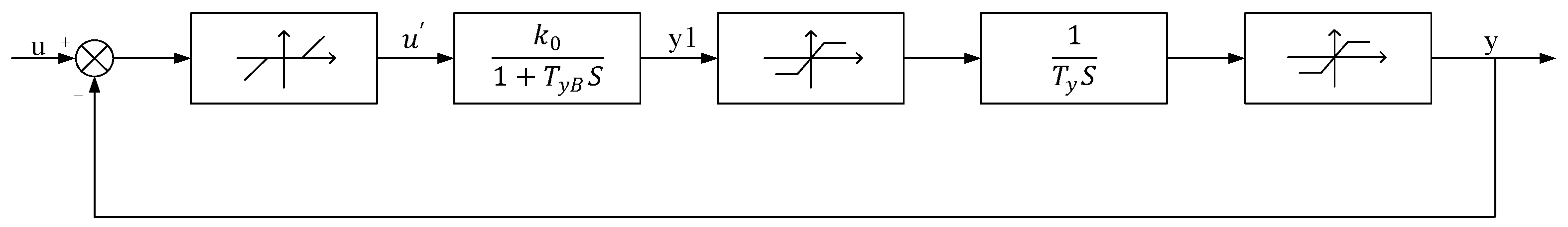
2.3. The Model of Servo Mechanism

According to the output $u$ controlled by the governor, the servo mechanism of the governor operates the guide vanes of the PSU to control the flow of the unit. The servo mechanism is composed of assistant servomotor and main servomotor. Due to the existence of a dead zone module and saturated zone module, it is a typical nonlinear link. The structure is shown in Figure 6.

$$\{\begin{array}{l}\frac{y_1(s)}{u(s)}=\frac{k_0}{1+T_{yb}s}\\ \frac{y(s)}{y_1(s)}=\frac{1}{T_{y}s}\end{array}$$

(13)

where $u_{}$ is the output signal of the controller; $k_0$ is the amplification factor; $T_{yb}$ is the time constant of the assistant servomotor; $T_y$ is the main servomotor time constant; $y_1$ is the main pressure valve opening; and $y_{}$ is the guide vane of the PSU.

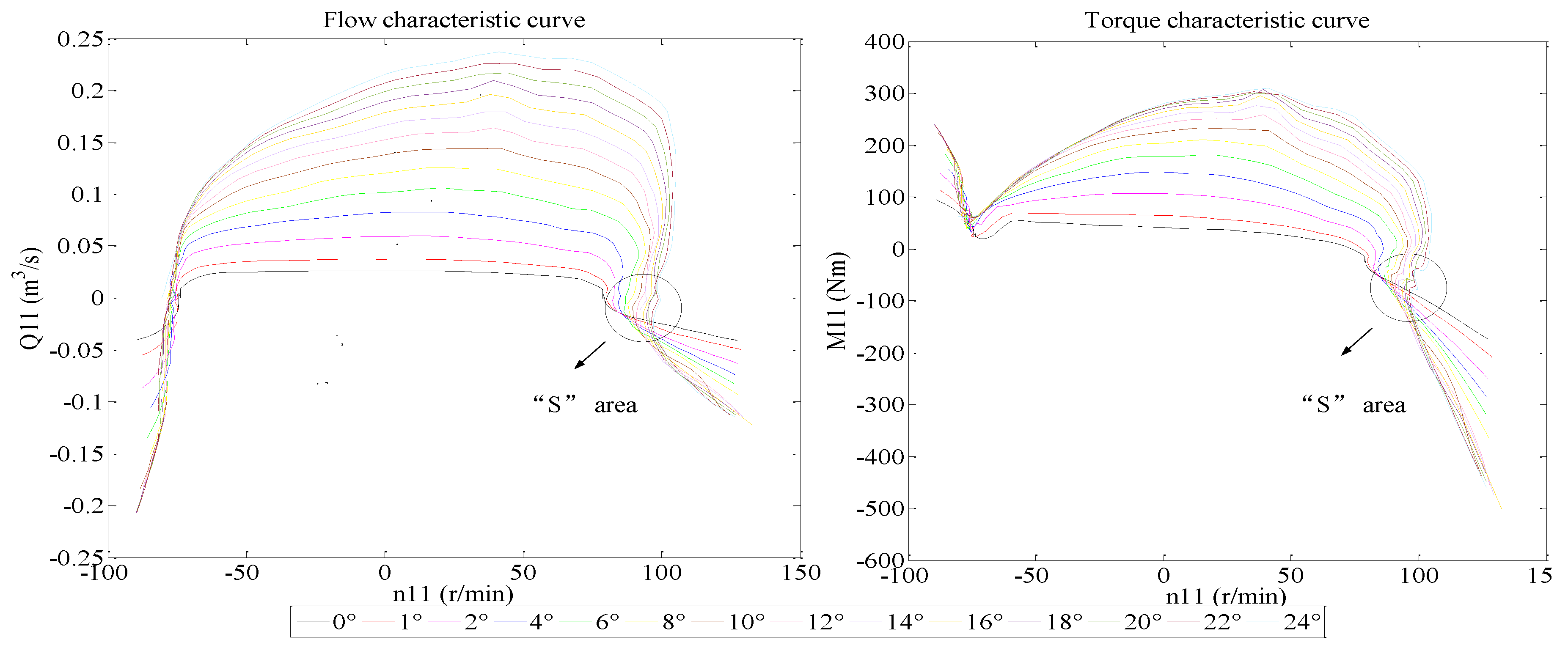
2.4. Model of the Pumped Storage Unit

There is a nonlinear relationship between the relative value of the change of the guide vane opening degree of the PSU and the relative value of the displacement of the servomotor. At present, no specific mathematical model can be established. Therefore, the simulation calculation of the PSU should be based on the full characteristic curve [36]. The full characteristic curve of the PSU is based on the vane opening $\theta$ as an intermediate variable to establish the flow characteristic curve $Q_{11}-N_{11}$ and torque characteristic curve $M_{11}-N_{11}$, as shown in Figure 7. The different combinations of these operating parameters divide the full characteristic curve into five operating conditions, including: The pump zone, the pump brake zone, the turbine zone, the turbine brake zone, and the reverse pump zone.

$$\{\begin{array}{l}{Q}_{11}=Q_{11}(\theta ,Q_{11})\\ M_{11}=M_{11}(\theta ,M_{11})\end{array}$$

(14)

When the frequency is adjusted in the working condition of the turbine, especially in the case of external load reduction under low water head, the unit speed of the turbine is shown as follows:

$$n_{11}=\frac{nD}{\sqrt{H}}$$

(15)

where $Q_{11}$ is the unit flow, $M_{11}$ is the unit torque, $n_{11}$ is the unit rotation speed, $n$ is the rotation speed, and $D$ is the nominal diameter of the PSU.

It can be seen from Figure 7 that the flow characteristic curve and torque characteristic curve of the PSU are overlapped and twisted in the area, with a relatively large rotational speed, which is the “S” characteristic area. The nominal diameter $D$ of the PSU is constant, and the reduction of external load leads to the increase of the unit rotation speed $n$. Then, the unit rotation speed $n_{11}$ with lower water head $H$ is relatively large, which makes the PSU easily run into the reverse pump zone under the influence of “S” characteristics, thus causing the rotation speed $n$ to fluctuate around the network frequency value.

In order to solve the single input–multiple out problem in “S” area, the Suter transformation method was adopted to convert the full characteristic curve of the PSU in the four quadrants into two inquire transformation curves. The transformed whole characteristic curve was transformed into $WM(x,y)$ and $WH(x,y)$ curves on the $x$ axis, but there were still some problems such as uneven opening distribution [37]. In view of the above problems, the improved Suter transformation was adopted [38]. The transformation relations are as follows.

$$\{\begin{array}{l}WH(x,y)=\frac{h}{a^2+q^2+C_{h}h}{(y+C_y)}^2\\ WM(x,y)=\frac{m+k_{2}h}{a^2+q^2+C_{h}h}{(y+C_y)}^2\end{array}$$

(16)

$$\{\begin{array}{l}a\ge 0,x=arctan\left[q+k_1\sqrt{h}/a\right]\\ a<0,x=\pi +arctan\left[q+k_1\sqrt{h}/a\right]\end{array}$$

(17)

where $a=\frac{n}{n_r}$; $q=\frac{Q}{Q_r}$; $m=\frac{M}{M_r}$; $h=\frac{H}{H_r}$; $k_1{}_{}$ is the coefficient, 0.5–1.2; $k_2>\frac{\left|M_{11\max }\right|}{M_{11}}$; $C_{y_1}$ is the coefficient, 0.1–0.3; $C_{y_2}$ is the coefficient, 0.4–0.6; and the subscript r represents the rating. According to the improved Suter transformation, the calculation model of pump turbine is expressed as follows:

$$\{\begin{array}{l}{h}_{n+1}=W_H(y_{n+1},x(q_{n+1},n_{n1}))\cdot (q_{n+1}^2+n_{n+1}^2)\\ m_{n+1}=W_M(y_{n+1},x(q_{n+1},n_{n1}))\cdot (q_{n+1}^2+n_{n+1}^2)\end{array}$$

(18)

In Equation (14), $h_1{}_1$ and $m_1{}_1$ represent the interpolation of the characteristic curve of the PSU. The improved Suter transformation can effectively solve the obstacle of single input–multiple output in the “S” area.

2.5. The Model of Generator and Loads Unit

The dynamic equilibrium relationship between the PSU’s active torque $m_t$ and the generator’s load torque $m_g$ is described by the motion equation [39]. According to the dynamic principle, the motion equation can be established as follows:

$$\frac{n(s)}{m_t(s)-m_g(s)}=\frac{1}{(T_{a}s+e_g)}$$

(19)

where $T_a$ is inertia time of the generator, and $e_g$ is the self-regulating coefficient of the generator.

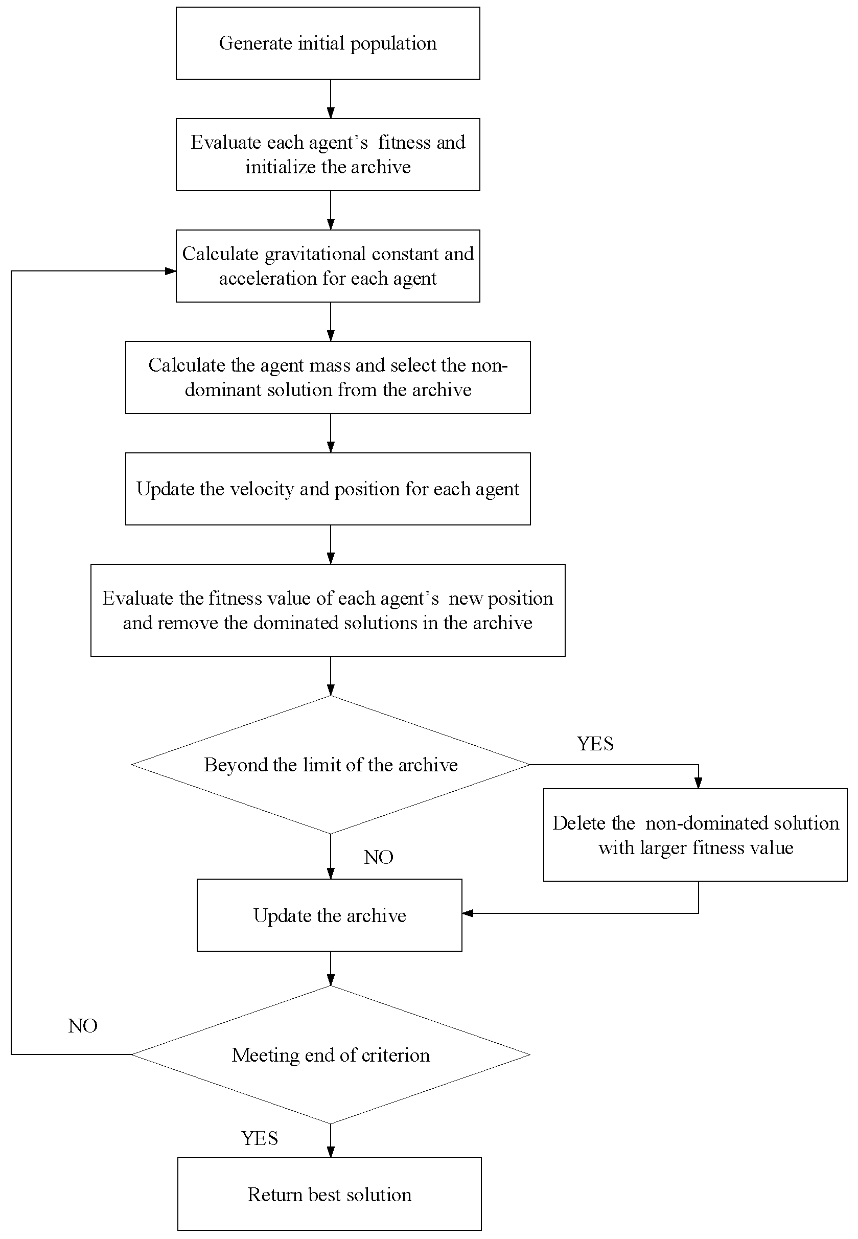
3. Multi-Objective Gravitational Search Algorithm (MOGSA)

3.1. MOGSA

3.1.1. Gravitational Search Algorithm (GSA)

The gravitational search algorithm (GSA) optimization algorithm mainly uses the gravity law between two objects to guide the motion of each particle to optimize the search for the optimal solution, the position of each particle corresponds to a solution to the problem. In the whole search space, the particle with the largest inertia mass represents the optimal solution to the problem. The optimization process of GSA is as follows.

Initialize each parameter and population position, suppose there is a particle in a separate system. Define the position of the particle as follows:

$$x_i=\left(x_i^1,x_i^d,\dots ,x_i^d,\dots ,x_i^n\right) for i=1,2,\dots ,N,$$

(20)

where $x_i^d$ is the position of the $i$th mass in $d$th dimension, and $N$ is the size of the population. The inertial mass is calculated by the fitness value of the particle:

$$\{\begin{array}{l}{m}_i(t)=\frac{fit(t)-wrost(t)}{best(t)-wrost(t)}\\ M_i(t)=\frac{m_i\left(t\right)}{{\displaystyle {\sum }_{j=1}^N{m}_j(t)}}\end{array}$$

(21)

where $fi{t}_i(t)$ represent the fitness value of the agent $i$ at the time $t$, the best and worst fitness values are defined below (for a minimization problem):

$$\{\begin{array}{l}best(t)=min fi{t}_j(t)\\ wrost(t)=max fi{t}_j(t)\end{array},j\in (1,\dots ,N)$$

(22)

Calculate the joint force of gravitation on the $d$th dimension space of $i$th agent at the time $t$:

$$F_i^d(t)={\displaystyle {\sum }_{j=1,j\ne i}^{N}rand\cdot F_{ij}^d(t)}$$

(23)

where $F_{ij}^d\left(t\right)$ is the magnitude of the gravitational force on particle $i$ from particle $j$ at $t$ moment.

$$F_i^d(t)=G(t)\frac{M_i(t)\cdot M_i(t)}{R_{ij}(t)+\epsilon }(x_j^d(t)-x_i^d(t))$$

(24)

where the $G\left(t\right)$ is the gravitational constant at t time, $R_{ij}$ is the distance between the $i$th agent and $d$th agent, $\mathsf{\epsilon }$ is a constant which is set for avoiding the divisor equal to zero.

$$G(t)=G(G_0,t)$$

(25)

$$R_{ij}(t)=|{|x}_i(t),x_j\left(t\right)|{|}_2$$

(26)

According to the law of motion, the acceleration $a_i^d(t)$ of agent $i$ at $t$ time, and in direction $d$th is given as follows:

$$a_i^d(t)=\frac{F_i^d(t)}{M_i(t)}$$

(27)

Then, calculate the velocity and position value of the agent $i$ at the next moment:

$$v_i^d(t+1)=ran{d}_i\cdot v_i^d(t)+a_i^d(t)$$

(28)

$$x_i^d(t+1)=x_i^d(t)+v_i^d(t+1)$$

(29)

3.1.2. Multi-Objective Optimization

Different from the single objective particle swarm optimization, the multi-objective particle swarm optimization has no single optimal solution, but a group of non-dominant solutions. The flowchart of the MOGSA algorithm is shown in Figure 8 and the detailed process of MOGSAs algorithm is as follows:

Step 1: Set the maximum number of iterations N, population size $nPop$, Pareto Front size $nRep$, dimension of search space D, and search space upper $S_{max}$ and lower limits $S_{min}$.

Step 2: The population positions randomly initialized in the search space and then the velocity vector corresponding to each particle is initialized to zero.

Step 3: Evaluate the fitness value of each agent on each object fitness function; next, update the archive which has a grid structure.

The grid structure is created as follows: Each dimension in the objective space is divided into equal divisions, where the agent $i$ denotes dimension index, and hence, for a k-objective optimization problem, there will be different segments.

Step 4: Update the gravitational constant the acceleration for each agent, calculate the mass (active mass) corresponding to each solution in the archive, and assign a uniform mass (passive mass) to the search particles.

Step 5: By calculating the agent mass, the optimal non-dominant solution is selected from the archive.

Step 6: For each individual population, update velocity and next position, respectively.

Step 7: Evaluate the fitness value of each agent’s new position. After, all of the new individuals are exposed to uniform mutation operator and those individuals among the resulting population, which is considered as non-dominated ones, are added to the archive. Finally, the keeping functionality removes those solutions that have recently become dominated in the archive.

Step 8: Update the archive and check the number of non-dominant solutions. If the number of elements in the archive gets to its limit, one of elements should be omitted from the archive.

Step 9: Determine whether the number of iterations N is reached; if the conditions are not met, loop operation Step 3–Step 9. Otherwise, output the non-dominant solution stored in the archive.

3.2. Objective Functions

In order to obtain controller optimization parameters that can satisfy the comprehensive index of the unit speed and the vane opening degree, two objective functions are set. The first objective function considers the integral time absolute error ($ITAE$) of rotational speed, oscillation level of the unit speed ($OUS$), and steady-state error ($SSE$) of the unit. The second objective function considers the ITAE of guide vane opening and the degree of oscillation of the vane opening ($OVO$). The integral of time multiplied absolute error $ITAE$ criterion is generally used to minimize time multiplied absolute error of the control system [40].

$$\{\begin{array}{l}{J}_1=ITA{E}_X+w_1\cdot OUS+w_2\cdot SSE\\ J_2=ITA{E}_y+w_3\cdot OVO\end{array}$$

(30)

where $OUS=Max(x)-Min(x)$; $SSE=x(N)-c$; $OVO=Max(y)-Min(y)$. $x(N)$ is the rotation speed of the unit after stabilization, $c$ is the rated speed. $Max(x)$ and $Min(x)$, respectively, represent the maximum and minimum values of the rotation speed in the adjustment process. $Max(y)$ and $Min(y)$, respectively, represent the maximum and minimum values of guide blade opening in the regulation process. $w_1$, $w_2$, and $w_3$ are weight coefficients to set the value of the different indexes within the same preset range. The importance of the three control indexes $ITA{E}_x$, $OUS$, and $SSE$ in $J_1$ and the two control indexes $ITA{E}_y$ and $OVO$ in $J_2$ have the same importance for the objective function value. Therefore, when selecting the weight coefficients of $w_1$,$w_2$, and $w_3$, matching with the magnitudes of $ITA{E}_x$ and $ITA{E}_y$ should be considered, so that the actual values of the five control indicators are of the same magnitude.

3.3. Optimization Variables

In order to obtain good stability in the regulation system, the controller parameters of the governor are usually optimized by the optimization algorithm. Therefore, this paper adopts the MOGSA algorithm to, respectively, optimize the parameters of PID control, FOPID controller, and FFOPID controller. The optimization variables of the different controllers are listed in

Table 4. Optimization variables of different controllers.

Controller	Optimization Variables
PID controller	$V_1=\left(K_p,K_i,K_d\right)$
FOPID controller	$V_2=\left(K_p,K_i,K_d,\mathsf{\lambda },\mathsf{\mu }\right)$
FPID controller	$V_3=\left(K_{p0},K_{i0},K_{d0}\right)$ $\mathit{center}=\left(ce{n}_p,ce{n}_i,ce{n}_d\right)$ $width=\left(\overrightarrow{wi{d}_p},\overrightarrow{wi{d}_i},\overrightarrow{wi{d}_d}\right)$
FFOPID controller	$V_4=\left(K_{p0},K_{i0},K_{d0},\mathsf{\lambda },\mathsf{\mu }\right)$ $\mathit{center}=\left(ce{n}_p,ce{n}_i,ce{n}_d\right)$ $width=\left(\overrightarrow{wi{d}_p},\overrightarrow{wi{d}_i},\overrightarrow{wi{d}_d}\right)$
Definition: PID is proportional-integral-derivative
Definition: FOPID is fractional-order proportional-integral-derivative
Definition: FPID is fuzzy proportional-integral-derivative
Definition: FFOPID is fuzzy fractional-order proportional-integral-derivative

.

4. Experiences and Results Analysis

In this section, the nonlinear model of the pumped storage unit regulating system with elastic water hammer effect was simulated in MATLAB. In order to show that the FFOPID controller has a better control effect than the traditional controller, they were successively put into the multiple simulation experiments for comparison.

4.1. Model Parameters

In the following simulation experiments, parameters of MOGSA were set as: $N$ = 100, $nPop$ = 50, $nRep$ = 30, G0 = 5, $nGrid$ = 10. Optimization variables were searched within specified ranges, the adopted search range for the PID controller parameters were restricted to $\left\{K_p,K_i,K_d\right\}$ ∈ $\left[0,8\right]$. For the FOPID controller, parameters were restricted to $\left\{K_p,K_i,K_d\right\}$ ∈ $\left[0,8\right]$, $\left\{\mathsf{\lambda },\mathsf{\mu }\right\}$ ∈ $\left[0,2\right]$. For the FPID controller, parameters were restricted to $\left\{K_{p0},K_{i0},K_{d0}\right\}$ ∈ $\left[0,8\right]$, $\left\{cen,\overrightarrow{wid}\right\}$ ∈ $\left[0,10\right]$. For the FFOPID controller, parameters were restricted to $\left\{K_{p0},K_{i0},K_{d0}\right\}$ ∈ $\left[0,8\right]$, $\left\{\mathsf{\lambda },\mathsf{\mu }\right\}$ ∈ $\left[0,2\right]$, and $\left\{cen,\overrightarrow{wid}\right\}$ ∈ $\left[0,10\right]$. The key parameters of the pumped storage unit regulating system are listed in

Table 5. Key parameters of the pumped storage unit regulating system.

Median servomotor response time $T_{y1}$	0.05
Primary servomotor response time $T_y$	0.3
Water head loss coefficient $f$	0.75
Water hammer pressure wave time constant $T_r$	1.0
Inertial time constant of generator $T_a$	8.503
Adjusting coefficient of generator $e_g$	0.1
Rated water head $H_w$	540.0

.

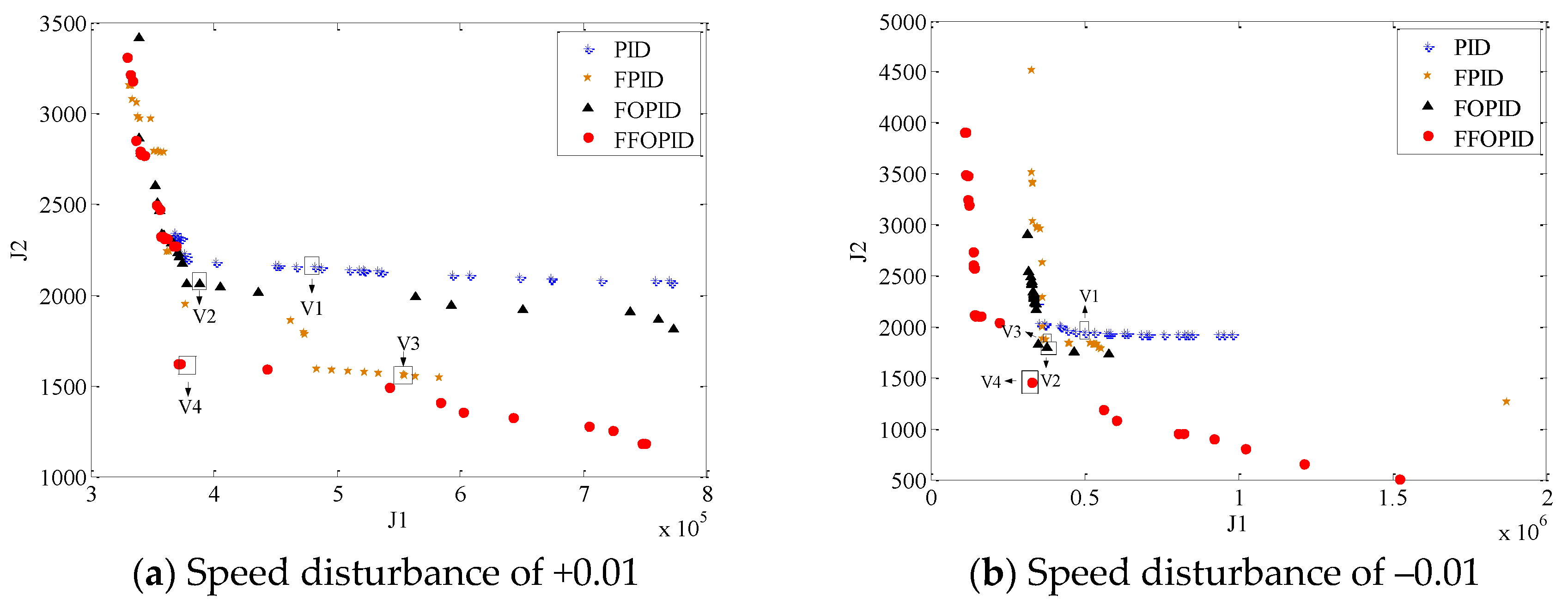
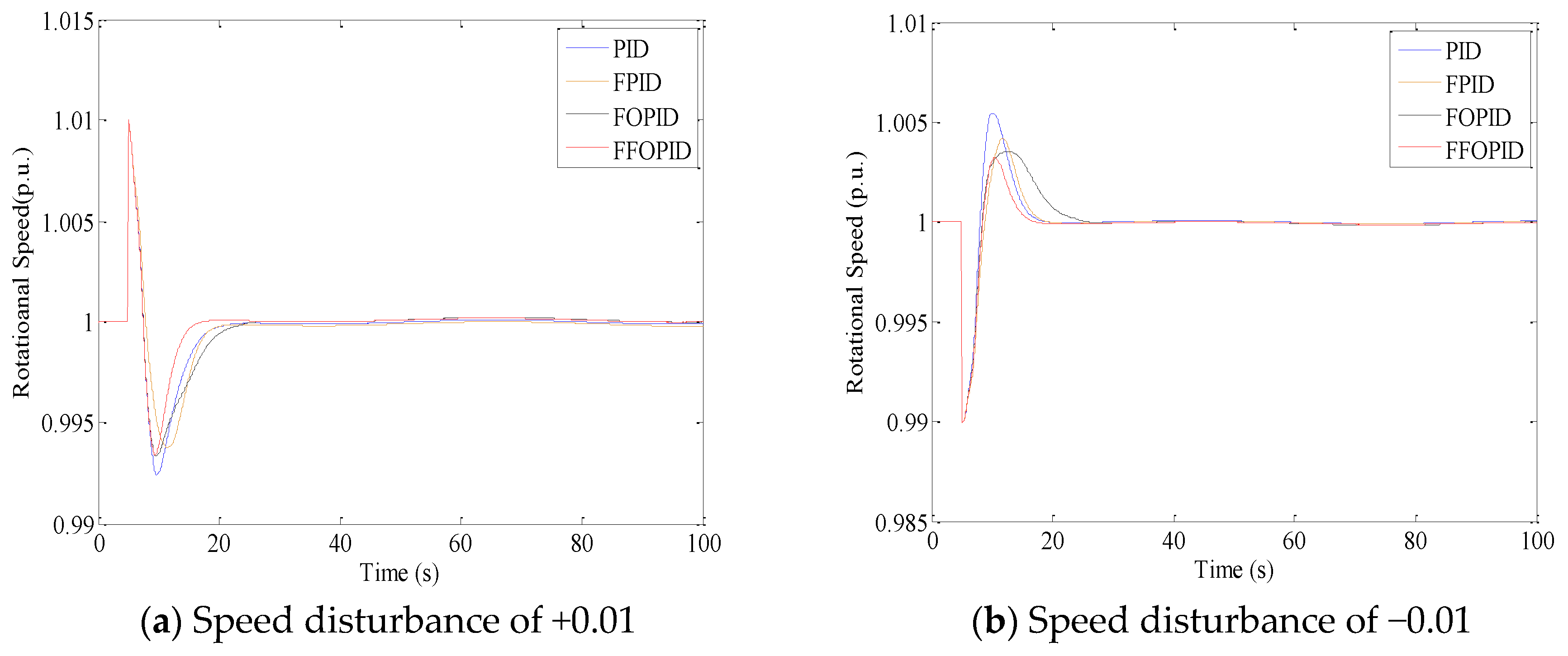
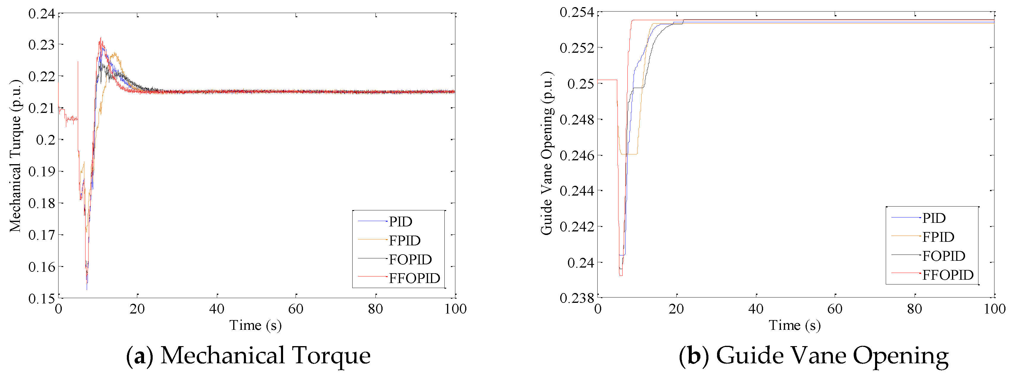
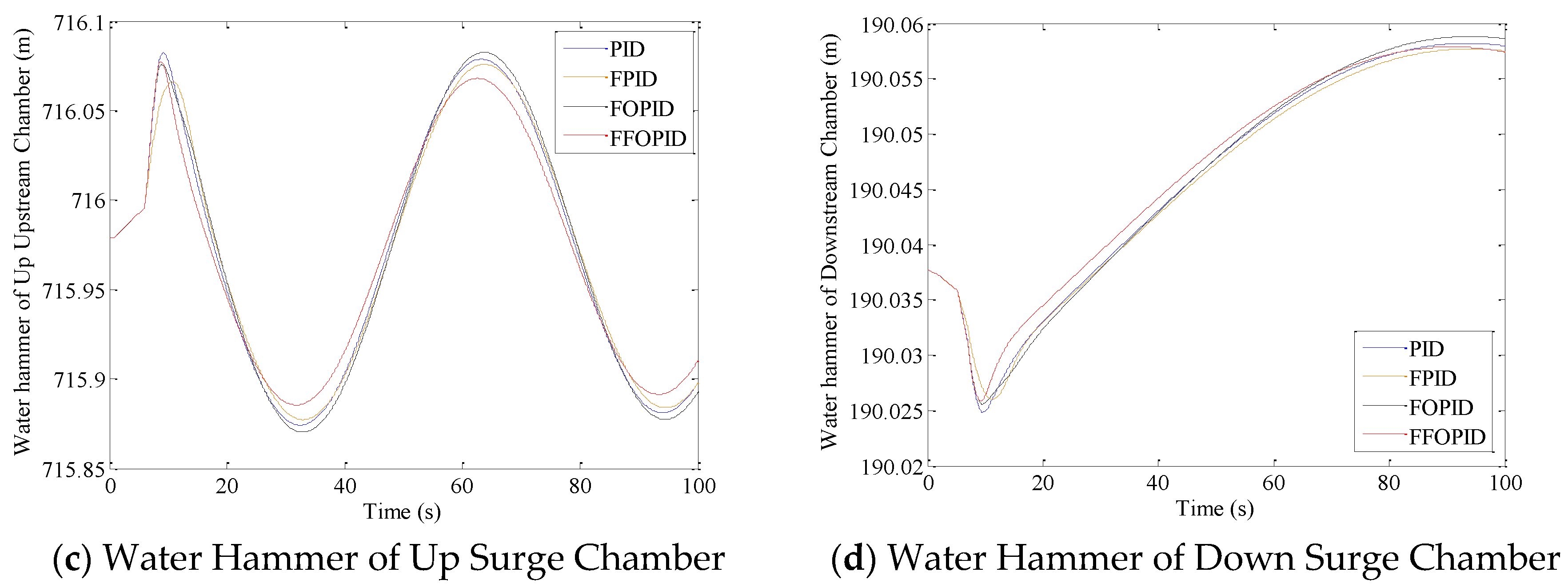
4.2. Comparison of the Performance of Different Controllers

In this part, the simulation experiments show that the pumped storage unit regulating system is assumed to be disturbed by frequency under the 25% guide vane opening condition at low water head. Furthermore, experiments were conducted under 526 m water head condition. The simulation time was 100 s, and the relative values of 0.01 and −0.01 speed disturbance were added at 5 s. Four sets of comparative experiments were carried out in the above conditions to compare the performance of the different controllers, and optimization parameters of the group that can obtain the best speed response curve were selected from the Pareto optimal solution set, respectively, as illustrated in Figure 9. The specific results of the optimization parameters are shown in

Table 6. Optimal parameters of controllers for pumped storage unit regulating system under rotational speed disturbance.

Speed Disturbance	Controller	Optimization Variables
+0.01	PID	$V_1=(1.3148,0.5117,1.5270)$
	FOPID	$V_2=(1.1553,0.9757,1.8070,1.1971,1.0196)$
	FPID	$V_3=(1.3948,0.4787,0.3977)$ ${center}_{best}=(5.5005,7.9525,0.9958)$ ${width}_{best}=\left(\begin{array}{ccc}9.1723& 6.0674& \begin{array}{cccc}5.7059& 8.5711& 5.0519& \begin{array}{cc}6.1979& 2.2455\end{array}\end{array}\\ 6.6428& 9.0604& \begin{array}{cccc}4.8956& 7.0170& 7.8289& \begin{array}{cc}6.4996& 6.9872\end{array}\end{array}\\ 5.7870& 9.8610& \begin{array}{cccc}5.2003& 5.8614& 8.8137& \begin{array}{cc}5.2139& 5.7073\end{array}\end{array}\end{array}\right)$
	FFOPID	$V_4=(1.7740,1.0148,2.0846,1.2810,1.1396)$ ${center}_{best}=(6.1071,8.6738,9.8692)$ ${width}_{best}=\left(\begin{array}{ccc}9.6735& 6.0843& \begin{array}{cccc}1.0731& 7.8910& 7.5085& \begin{array}{cc}7.7632& 8.5078\end{array}\end{array}\\ 6.0727& 6.6815& \begin{array}{cccc}3.6551& 9.0820& 6.7214& \begin{array}{cc}6.7312& 4.9343\end{array}\end{array}\\ 4.1924& 7.7019& \begin{array}{cccc}8.7038& 5.1356& 9.2576& \begin{array}{cc}9.6115& 9.4028\end{array}\end{array}\end{array}\right)$
−0.01	PID	$V_1=(2.1505,0.8765,2.0909)$
	FOPID	$V_2=(1.1099,0.9354,1.7472,1.1674,1.0165)$
	FPID	$V_3=(2.0945,0.4879,1.6760)$ ${center}_{\mathrm{best}}=(7.7436,9.7880,9.1701)$ ${width}_{best}=\left(\begin{array}{ccc}\begin{array}{ccc}6.0918& 3.3666& 9.9720\end{array}& 1.2646& \begin{array}{cc}1.1026& \begin{array}{cc}6.4191& 3.3703\end{array}\end{array}\\ \begin{array}{ccc}9.4954& 3.7979& 9.9760\end{array}& 9.7331& \begin{array}{cc}2.7428& \begin{array}{cc}2.2519& 6.4656\end{array}\end{array}\\ \begin{array}{ccc}5.6639& 1.8315& 9.4198\end{array}& 2.3303& \begin{array}{cc}4.8298& \begin{array}{cc}8.5215& 9.6070\end{array}\end{array}\end{array}\right)$
	FFOPID	$V_4=(2.1915,0.9876,2.0599,1.2133,1.0548)$ ${center}_{best}=(9.1896,6.4108,8.3543)$ ${width}_{best}=\left(\begin{array}{ccc}\begin{array}{ccc}9.8247& 5.4821& 5.3268\end{array}& 5.5733& \begin{array}{cc}3.8928& \begin{array}{cc}9.8321& 8.2310\end{array}\end{array}\\ \begin{array}{ccc}8.0921& 2.4436& 3.0347\end{array}& 8.8413& \begin{array}{cc}5.5852& \begin{array}{cc}5.1895& 6.3547\end{array}\end{array}\\ \begin{array}{ccc}9.3628& 4.3806& 5.1396\end{array}& 4.8648& \begin{array}{cc}9.5264& \begin{array}{cc}9.8260& 5.0988\end{array}\end{array}\end{array}\right)$

, and Figure 10 shows the membership function of the output variable optimized by the MOGSA algorithm.

The comparison of speed curves is shown in Figure 11. It can be seen from Figure 11 that when the speed disturbance occurs, the response curve with the FFOPID controller fluctuates less and the adjustment time is shorter. In order to show the optimization effect of the FFOPID controller, the experimental results of control indices are shown in

Table 7. Control indices of controllers for pumped storage unit regulating system under rotational speed disturbance.

Speed Disturbance	Controller	$\mathit{J}{1}_{\mathit{m}\mathit{i}\mathit{n}}\left(\times 10^5\right)$	$\mathit{J}{2}_{\mathit{m}\mathit{i}\mathit{n}}\left(\times 10^3\right)$	$\mathit{I}\mathit{T}\mathit{A}{\mathit{E}}_{\mathit{x}}$	$\mathit{I}\mathit{T}\mathit{A}{\mathit{E}}_{\mathit{y}}$	$\mathit{O}\mathit{U}\mathit{S}$	$\mathit{S}\mathit{t}\mathit{a}\mathit{b}\mathit{l}\mathit{e} \mathit{T}\mathit{i}\mathit{m}\mathit{e}(\mathit{s})$
+0.01	PID	4.821	2.155	43.74	120.17	0.0176	11.48
	FPID	5.55	1.55	52.84	99.89	0.0162	11.94
	FOPID	3.884	2.061	59.03	152.10	0.0167	13.44
	FFOPID	3.772	1.623	42.54	143.14	0.0166	8.66
–0.01	PID	5.016	1.948	31.76	122.47	0.0155	9.52
	FPID	3.753	1.870	32.56	112.09	0.0142	10.54
	FOPID	3.792	1.793	43.79	111.96	0.0135	12.98
	FFOPID	3.299	1.458	28.45	99.59	0.0133	8.32

. By comparing the corresponding control indices of the PID controller, FOPID controller, FPID controller, and FFOPID controller, the performance of these controllers can be fully displayed. It can be seen from Table 7 that when the PSU is disturbed by the relative speeds of 0.01 and −0.01 under the FFOPID controller, the control indexes $ITA{E}_x$ are 42.54 and 28.45, respectively, which are smaller than other controllers. The smaller $ITA{E}_x$ indicates that the speed curve of the PSU has better dynamic characteristics. From Figure 11, it can be seen that when the PSU is disturbed in 5 s, the speed curve enters into the oscillation area. Under the action of the FFOPID controller, the speed fluctuation is small, and the control index OUS value is lower than that of the traditional controller. According to the regulation time, the stability time values of the two disturbances are 8.66 s and 8.32 s, respectively, which are far less than the PID, FOPID, and FPID controllers. These indices show that the FFOPID controller is more suitable for improving the control performance of the nonlinear pumped storage unit regulating system with elastic water hammer effect, compared with other controllers.

The transient processes of the pumped storage unit regulating with different controllers corresponding to rotational speed disturbance of 0.01 are shown in Figure 12, in which mechanical torque, guide vane opening, and characteristic curves of the water hammer of the surge chamber can be seen.

As shown in Figure 12a, the FFOPID controller can control the mechanical torque to a stable state faster than the PID controller and FOPID controller. It can also be seen from Figure 12b that under the action of the FFOPID controller, the guide blade opening can be balanced quickly and rapidly, so the corresponding rotational speed curve first reaches a stable state. Therefore, it can be considered that the FFOPID controller is better. Meanwhile, the results show that the oscillation amplitude of the water hammer in the surge chamber obtained by the FFOPID controller is smaller than that obtained by other controllers, as shown in Figure 12c,d. The above conclusion indicates that the FFOPID controller can provide more stable operating conditions.

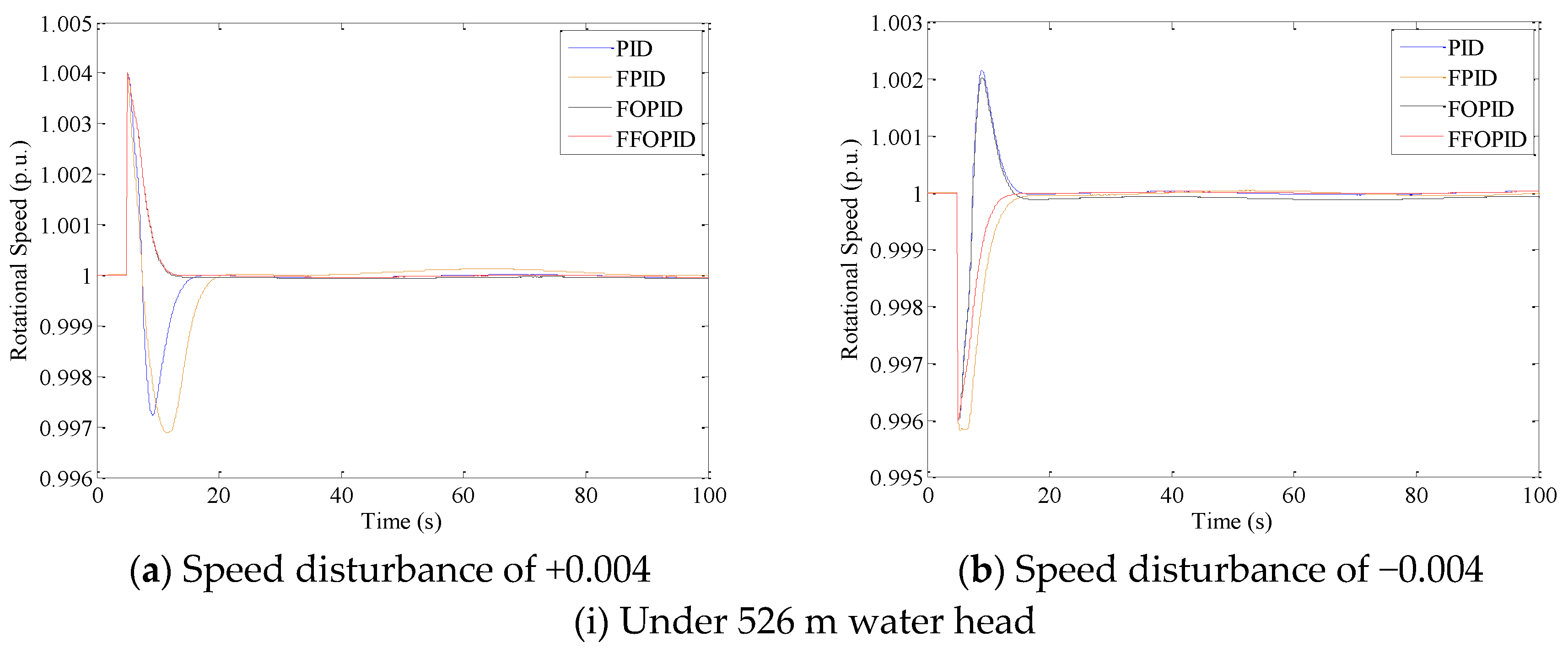
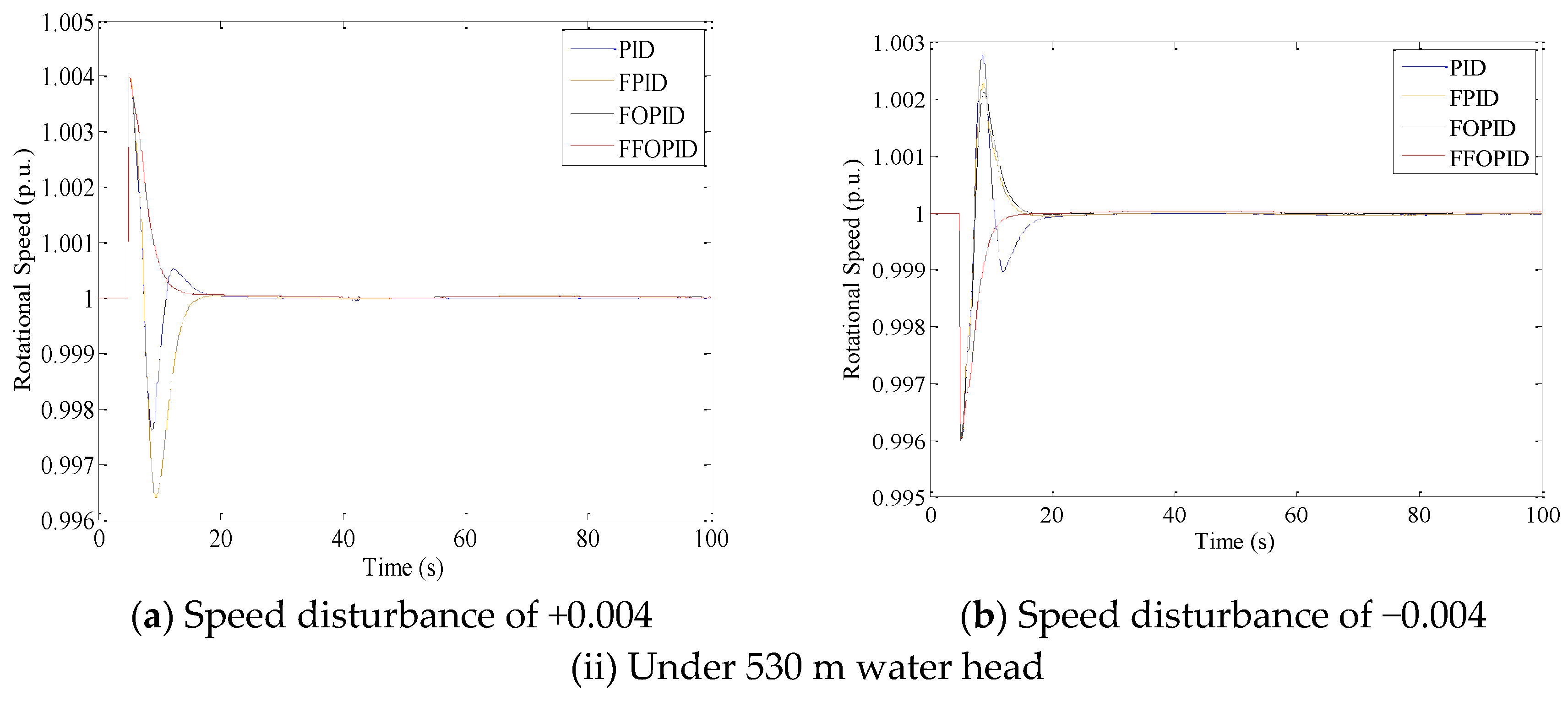
4.3. Robustness Analysis of the Proposed Method

The low-frequency disturbance is the key factor to the stability of the pumped storage unit regulating system under the condition of low water head. Furthermore, the water hammer effect caused by the controller’s poor robustness is an important cause of PSU vibration. Therefore, in this paper, the robustness test of the FFOPID controller was carried out by adjusting the value of a rotational speed disturbance of 0.004, −0.004. Figure 13, respectively, gives the rotational speed response of the pumped storage unit regulating system when subjected to low-frequency disturbance at 526 m and 530 m water head during operation. It can be seen that the control performance of the FFOPID controller under low-speed disturbance is obviously better than that of traditional controllers. The experimental results show that the proposed FFOPID controller of the pumped storage unit regulating system shows sufficient robustness to hydraulic parameter variation of the system under primary frequency modulation.

5. Conclusions

In order to improve the stability of the pumped storage unit regulating system when it encounters rotation speed disturbance in low water head operation, this paper presented an FFOPID controller based on the fuzzy theory and FOPID controller. Furthermore, a multi-objective optimization strategy combining fuzzy rules and control parameters was applied to the primary frequency regulation of the pumped storage unit regulating system. In the simulation experiment, the FFOPID controller was compared with the FOPID controller, PID controller, and FPID controller. In order to verify its robustness, different speed disturbance tests were carried out under the condition of low water head. The experimental analysis results indicated that the FFOPID controller could effectively restrain the oscillation of rotational speed at low water head. In future work, we will apply the FFOPID controller to more operating conditions of the pumped storage unit regulating system to verify its control performance.

References

1. Lai, X.; Li, C.; Zhou, J.; Zhang, N. Multi-objective optimization of the closure law of guide vanes for pumped storage units. Renew. Energy 2019, 139, 302–312. [Google Scholar] [CrossRef]
2. Rehman, S.; Al-Hadhrami, L.M.; Alam, M.M. Pumped hydro energy storage system: A technological review. Renew. Sustain. Energy Rev. 2015, 44, 586–598. [Google Scholar] [CrossRef]
3. Xu, Y.; Li, C.; Wang, Z.; Nan, Z.; Bing, P. Load frequency control of a novel renewable energy integrated micro-grid containing pumped hydropower energy storage. IEEE Access 2018, 6, 29067–29077. [Google Scholar] [CrossRef]
4. Zhang, Z.; Yan, K.; Ge, W.; Yuan, J.; Shen, L.; Wang, S.J.; Liu, Q.; Pan, D.; Zhang, X. Research on Primary Frequency Modulation Strategy of Hydropower Unit; IEEE: New York, NY, USA, 2018; pp. 214–219. [Google Scholar]
5. Chandrakala, V.; Sukumar, B.; Sankaranarayanan, K. Load Frequency Control of Multi-source Multi-area Hydro Thermal System Using Flexible Alternating Current Transmission System Devices. Electr. Power Compon. Syst. 2014, 42, 927–934. [Google Scholar] [CrossRef]
6. Hu, Z.X.; Wang, Y.; Ge, M.F.; Liu, J. Data-driven Fault Diagnosis Method based on Compressed Sensing and Improved Multi-scale Network. IEEE Trans. Ind. Electron. 2020, 67, 3216–3225. [Google Scholar] [CrossRef]
7. Wu, W. Primary frequency modulation performance optimization of large pumped storage unit. Electron. Test 2015, 23, 119–120. [Google Scholar]
8. Li, C.; Zhang, N.; Lai, X.; Zhou, J.; Xu, Y. Design of a fractional-order PID controller for a pumped storage unit using a gravitational search algorithm based on the Cauchy and Gaussian mutation. Inf. Sci. 2017, 396, 162–181. [Google Scholar] [CrossRef]
9. Zhao, Z.G.; Yang, J.D.; Yang, W.J.; Hu, J.H.; Chen, M. A coordinated optimization framework for flexible operation of pumped storage hydropower system: Nonlinear modeling, strategy optimization and decision making. Energy Conv. Manag. 2019, 194, 75–93. [Google Scholar] [CrossRef]
10. Zhou, J.X.; Cai, F.L.; Wang, Y. New Elastic Model of Pipe Flow for Stability Analysis of the Governor-Turbine-Hydraulic System. J. Hydraul. Eng. ASCE 2011, 137, 1238–1247. [Google Scholar] [CrossRef]
11. Sun, H.; Xiao, R.; Liu, W.; Wang, F. Analysis of S Characteristics and Pressure Pulsations in a Pump-Turbine With Misaligned Guide Vanes. J. Fluids Eng. 2013, 135, 511011. [Google Scholar] [CrossRef]
12. Yang, W.J.; Norrlund, P.; Bladh, J.; Yang, J.D.; Lundin, U. Hydraulic damping mechanism of low frequency oscillations in power systems: Quantitative analysis using a nonlinear model of hydropower plants. Appl. Energy 2018, 212, 1138–1152. [Google Scholar] [CrossRef]
13. Yang, W.J.; Yang, J.D.; Zeng, W.; Tang, R.B.; Hou, L.Y.; Ma, A.T.; Zhao, Z.G.; Peng, Y.M. Experimental investigation of theoretical stability regions for ultra-low frequency oscillations of hydropower generating systems. Energy 2019, 186, 12. [Google Scholar] [CrossRef]
14. Li, C.S.; Mao, Y.F.; Zhou, J.Z.; Zhang, N.; An, X.L. Design of a fuzzy-PID controller for a nonlinear hydraulic turbine governing system by using a novel gravitational search algorithm based on Cauchy mutation and mass weighting. Appl. Soft Comput. 2017, 52, 290–305. [Google Scholar] [CrossRef]
15. Mohanty, P.K.; Sahu, B.K.; Pati, T.K.; Panda, S.; Kar, S.K. Design and analysis of fuzzy PID controller with derivative filter for AGC in multi-area interconnected power system. IET Gener. Transm. Distrib. 2016, 10, 3764–3776. [Google Scholar] [CrossRef]
16. Sahu, B.K.; Pati, T.K.; Nayak, J.R.; Panda, S.; Kar, S.K. A novel hybrid LUS-TLBO optimized fuzzy-PID controller for load frequency control of multi-source power system. Int. J. Electr. Power Energy Syst. 2016, 74, 58–69. [Google Scholar] [CrossRef]
17. Xu, Y.; Zheng, Y.; Du, Y.; Yang, W.; Peng, X.; Li, C. Adaptive condition predictive-fuzzy PID optimal control of start-up process for pumped storage unit at low head area. Energy Convers. Manag. 2018, 177, 592–604. [Google Scholar] [CrossRef]
18. Wang, B.; Shi, K.; Yang, L.; Wu, F.; Chen, D. Fuzzy generalised predictive control for a class of fractional-order non-linear systems. IET Control Theory Appl. 2018, 12, 87–96. [Google Scholar] [CrossRef]
19. Zamani, A.; Barakati, S.M.; Yousofi-Darmian, S. Design of a fractional order PID controller using GBMO algorithm for load–frequency control with governor saturation consideration. ISA Trans. 2016, 64, 56–66. [Google Scholar] [CrossRef]
20. Arya, Y.; Kumar, N. BFOA-scaled fractional order fuzzy PID controller applied to AGC of multi-area multi-source electric power generating systems. Swarm Evol. Comput. 2016, 32, 202–218. [Google Scholar] [CrossRef]
21. Chen, S.; Zhongning, H.E.; Zhou, Z.; Pan, G.; Yan, D. Study on transient process of low water-head large pumping station while pumping off. J. Hydroelectr. Eng. 2007, 26, 128–133. [Google Scholar]
22. Yang, W.; Yang, J. Study on optimum start-up method for hydroelectric generating unit based on analysis of the energy relation. In Proceedings of the 2012 Asia-Pacific Power and Energy Engineering Conference, Shanghai, China, 27–29 March 2012. [Google Scholar]
23. Bhattacharya, A.; Roy, P.K. Solution of multi-objective optimal power flow using gravitational search algorithm. IET Gener. Transm. Distrib. 2012, 6, 751–763. [Google Scholar] [CrossRef]
24. Nobahari, H.; Nikusokhan, M.; Siarry, P. A Multi-Objective Gravitational Search Algorithm Based on Non-Dominated Sorting. Int. J. Swarm Intell. Res. IJSIR 2012, 3, 32–49. [Google Scholar] [CrossRef] [Green Version]
25. Tawhid, M.A.; Savsani, V. A novel multi-objective optimization algorithm based on artificial algae for multi-objective engineering design problems. Appl. Intell. 2018, 48, 3762–3781. [Google Scholar] [CrossRef]
26. Hemmatian, H.; Fereidoon, A.; Assareh, E. Optimization of hybrid laminated composites using the multi-objective gravitational search algorithm (MOGSA). Eng. Optim. 2014, 46, 1169–1182. [Google Scholar] [CrossRef]
27. Moghadam, M.S.; Nezamabadi-Pour, H.; Farsangi, M.M. A Quantum Behaved Gravitational Search Algorithm. Intell. Inf. Manag. 2012, 4, 390–395. [Google Scholar] [CrossRef] [Green Version]
28. Wyrzykowski, L.; Udalski, A.; Kubiak, M.; Szymanski, M.; Zebrun, K.; Soszynski, I.; Wozniak, P.R.; Pietrzynski, G.; Szewczyk, O. The Optical Gravitational Lensing Experiment. Eclipsing Binary Stars in the Large Magellanic Cloud. J. Physiol. 2003, 340, 195–208. [Google Scholar]
29. Naserbegi, A.; Aghaie, M.; Minuchehr, A.; Alahyarizadeh, G. A novel exergy optimization of Bushehr nuclear power plant by gravitational search algorithm (GSA). Energy 2018, 148, 373–385. [Google Scholar] [CrossRef]
30. Assareh, E.; Biglari, M. A novel approach to capture the maximum power from variable speed wind turbines using PI controller, RBF neural network and GSA evolutionary algorithm. Renew. Sustain. Energ. Rev. 2015, 51, 1023–1037. [Google Scholar] [CrossRef]
31. Xu, Y.; Zhou, J.; Xue, X.; Fu, W.; Zhu, W.; Li, C. An adaptively fast fuzzy fractional order PID control for pumped storage hydro unit using improved gravitational search algorithm. Energy Convers. Manag. 2016, 111, 67–78. [Google Scholar] [CrossRef]
32. Afshar, M.H.; Rohani, M. Water hammer simulation by implicit method of characteristic. Int. J. Press. Vessel. Pip. 2008, 85, 851–859. [Google Scholar] [CrossRef]
33. Sim, W.G.; Park, J.H. Transient analysis for compressible fluid flow in transmission line by the method of characteristics. KSME Int. J. 1997, 11, 173–185. [Google Scholar] [CrossRef]
34. Zamani, M.; Karimi-Ghartemani, M.; Sadati, N.; Parniani, M. Design of a fractional order PID controller for an AVR using particle swarm optimization. Control Eng. Pract. 2009, 17, 1380–1387. [Google Scholar] [CrossRef]
35. Oustaloup, A.; Levron, F.; Mathieu, B.; Nanot, F.M. Frequency-band complex noninteger differentiator: Characterization and synthesis. IEEE Trans. Circuits Syst. I Fundam. Theory Appl. 2000, 47, 25–39. [Google Scholar] [CrossRef]
36. Hou, J.J.; Li, C.S.; Tian, Z.Q.; Xu, Y.H.; Lai, X.J.; Zhang, N.; Zheng, T.P.; Wu, W. Multi-Objective Optimization of Start-up Strategy for Pumped Storage Units. Energies 2018, 11, 1141. [Google Scholar] [CrossRef] [Green Version]
37. Suter, P. Representation of pump characteristic for calculation of water hammer. Sulzer Tech. Rev. 1966, 66, 45–48. [Google Scholar]
38. Zheng, X.B.; Guo, P.C.; Tong, H.Z.; Luo, X.Q. Improved Suter-transformation for complete characteristic curves of pump-turbine. IOP Conf. Ser. Earth Environ. Sci. 2012, 15, 062015. [Google Scholar] [CrossRef]
39. Yang, W.J.; Yang, J.D.; Guo, W.C.; Zeng, W.; Wang, C.; Saarinen, L.; Norrlund, P. A Mathematical Model and Its Application for Hydro Power Units under Different Operating Conditions. Energies 2015, 8, 10260–10275. [Google Scholar]
40. Pan, I.; Das, S.; Gupta, A. Tuning of an optimal fuzzy PID controller with stochastic algorithms for networked control systems with random time delay. ISA Trans. 2011, 50, 28–36. [Google Scholar] [CrossRef]
Figure 1. The structure of a pumped storage unit regulating system.
Energies 13 00137 g001
Figure 2. Force diagram of the micro-water body in the pressure pipeline.
Energies 13 00137 g002
Figure 3. Water hammer characteristic lines in the xt coordinate system.
Energies 13 00137 g003
Figure 4. The structure of the fuzzy fractional-order PID controller.
Energies 13 00137 g004
Figure 5. Membership functions of input variables and output variables.
Energies 13 00137 g005
Figure 6. Structure of servo mechanism.
Energies 13 00137 g006
Figure 7. The characteristic curves of pump turbine.
Energies 13 00137 g007
Figure 8. Flowchart of the multi-objective gravitational search algorithm (MOGSA).
Energies 13 00137 g008
Figure 9. Pareto optimal solutions obtained through MOGSA for speed disturbance of +0.01 and −0.01 under 526 m low water head.
Energies 13 00137 g009
Figure 10. Optimal membership function by MOGSA.
Energies 13 00137 g010aEnergies 13 00137 g010b
Figure 11. Comparison of speed curves by different controllers.
Energies 13 00137 g011
Figure 12. Transient processes of the pumped storage unit (PSU) with different controllers: (a) Mechanical Torque; (b) Guide Vane Opening; (c) Water Hammer of Up Surge Chamber; (d) Water Hammer of Down Surge Chamber.
Energies 13 00137 g012aEnergies 13 00137 g012b
Figure 13. Robustness of the FFOPID controller for variation in rotational speed disturbance.
Energies 13 00137 g013aEnergies 13 00137 g013b