Fig Plant Segmentation from Aerial Images Using a Deep Convolutional Encoder-Decoder Network

Abstract

Crop segmentation is an important task in Precision Agriculture, where the use of aerial robots with an on-board camera has contributed to the development of new solution alternatives. We address the problem of fig plant segmentation in top-view RGB (Red-Green-Blue) images of a crop grown under open-field difficult circumstances of complex lighting conditions and non-ideal crop maintenance practices defined by local farmers. We present a Convolutional Neural Network (CNN) with an encoder-decoder architecture that classifies each pixel as crop or non-crop using only raw colour images as input. Our approach achieves a mean accuracy of 93.85% despite the complexity of the background and a highly variable visual appearance of the leaves. We make available our CNN code to the research community, as well as the aerial image data set and a hand-made ground truth segmentation with pixel precision to facilitate the comparison among different algorithms.

1. Introduction

Precision Agriculture or Smart Farming aims to increase crop yield, reduce production costs and decrease environmental impact. In this context, an active research area is to identify crops automatically in digital images to classify plants, to monitor its growth or to detect problems of water stress, nutrition or health in cultivated plants. This problem is complicated under open field cultivation due to different factors such as natural lighting, weather and agricultural practices of the farmers.

The research carried out so far has been limited only to cases where the open field crops have small plants that are well separated from one another, the colour of the soil with respect to the plants is very different and the overlap among leaves of the same plant occurs very rarely [1,2,3]. Moreover, the state-of-the-art has focused on annual crops with careful cultivation techniques, without addressing the accurate segmentation case of fig (Ficus carica) perennial plants in an orchard where their particular characteristics [4] cause complex image patterns.

Leaves and fruits of fig have several nutritional and medicinal properties and currently the interest in its production has increased worldwide [5]. According to FAOSTAT report 2016, the harvested area of fig in the world was estimated around 308,460 hectares with a production of 1,050,459 tons [6]. The top five producers are Turkey, Egypt, Algeria, Iran and Morocco. In the case of México, the fig export market has been recently opened for the United States, which foresees an increase of fig planted area. In 2015, the cultivation area was about 1199 hectares yielding a total of 5381 tons with a value of approximately US$ 2,839,500.00 [7].

On the other hand, Unmanned Aerial Vehicles (UAVs) have many characteristics that make them attractive elements for precision agriculture [8]. UAVs can continuously travel large tracts of cultivated land in a short time and they have the capacity to carry light-weight compact sensors to capture information at low altitude. The RGB (Red-Green-Blue) cameras are one of the most used sensors in UAVs since they are relatively cheap, have low energy consumption and are light. It is true that multispectral or thermal cameras have been extensively used to vegetation monitoring [9,10], however these cameras are more expensive compared to RGB cameras.

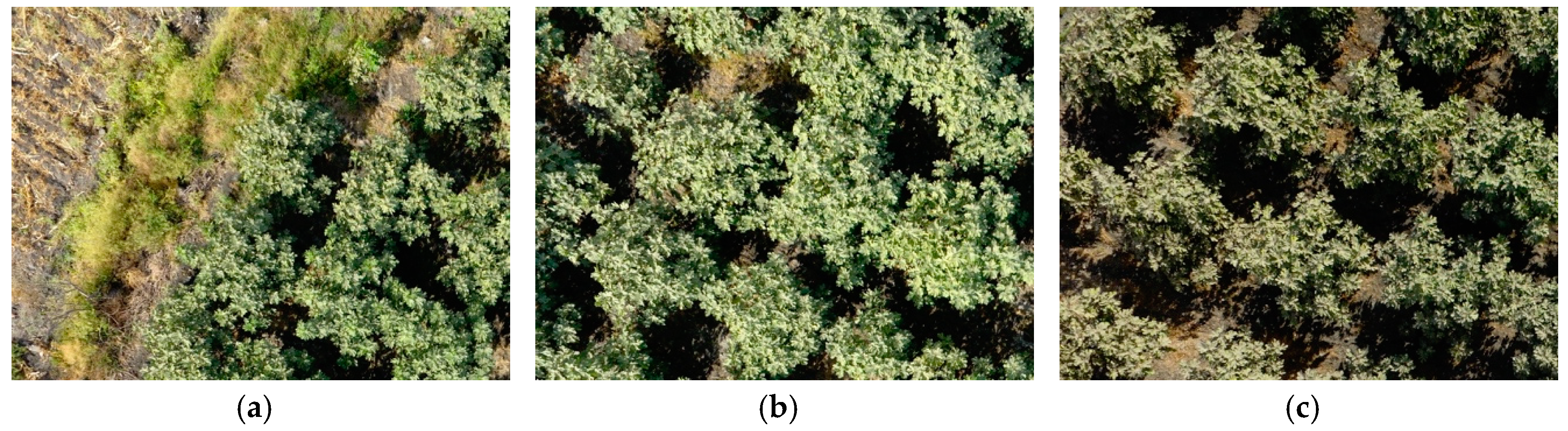
In this paper, we address the problem of crop segmentation at pixel level. Our approach exploits relevant information from high resolution RGB images captured by an UAV in a difficult open field environment. Indeed, we are considering realistic environmental conditions where there are illumination variations and different types of soil and weed, most treetops are overlapping, the inter-row space of field crop is not constant and there may be various elements that are not of interest, for example, stones or objects used by farmers. Furthermore, we deal with the specific case of a crop of woody and tall fig plants, which leads to additional problems in top-view images. The branches of fig plants grow around and along the stem and their leaves are divided into 7 lobes. 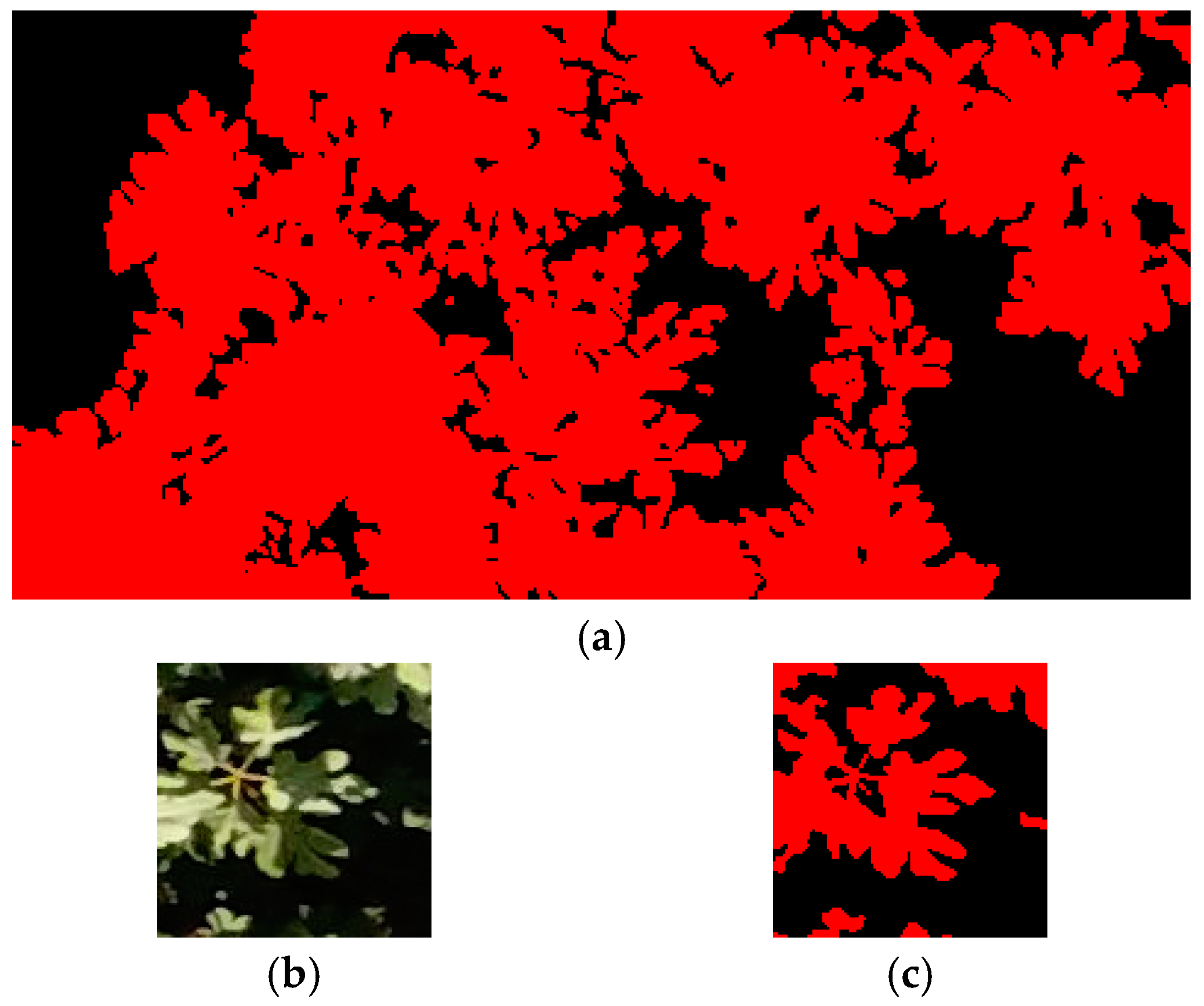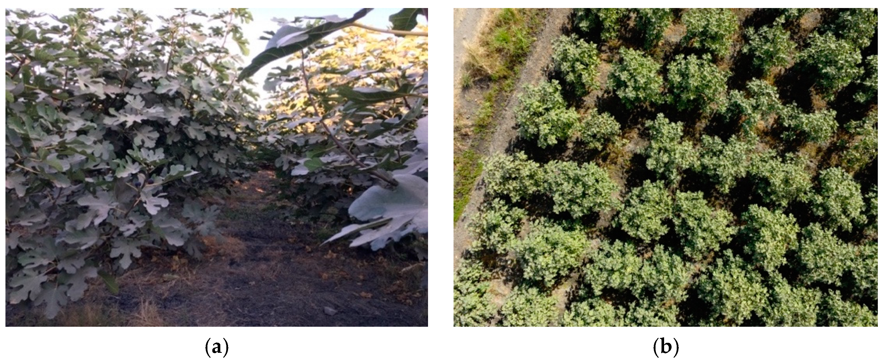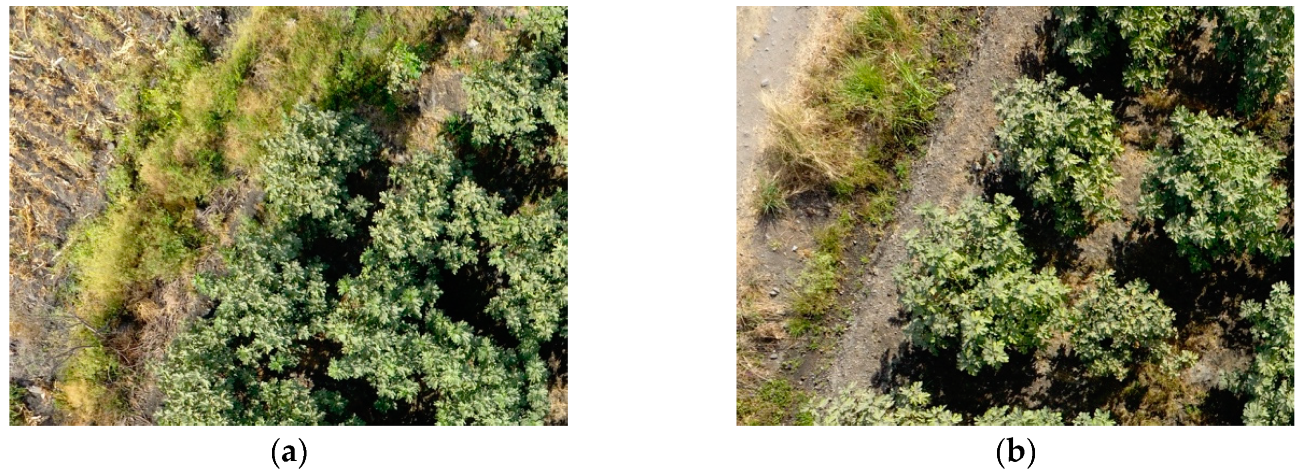Figure 1 shows examples of ground and aerial views of fig shrubs in which the plant morphology and the cultivation conditions are appreciated. Factors like camera position, solar illumination and plant morphology originate a visual appearance of the leaves that is drastically variable due to the formation of specularities, shadows, occlusions and different shapes, even though they have been captured at the same time in the morning.

We propose the use of a Convolutional Neural Network (CNN) with an encoder-decoder architecture trained end-to-end as the means to address the problem of plant segmentation at the granularity of pixel. Since artificial neural networks are highly robust approximation functions [11], which when used with convolutional layers have set the state-of-the-art for dealing with different image-related tasks [12,13,14], it is reasonable to expect that they could be used to perform segmentation in such a challenging scenario as ours. Furthermore, an encoder-decoder architecture provides the tools required to map RGB images onto binary images corresponding to segmentation indicator. Our model allows to classify each pixel of an image into crop or non-crop by using only the raw RGB pixel intensity values as input. In addition, we present an evaluation of algorithms based on the RGB colour model to detect vegetation, classical algorithms that have been considered as a reference for this type of analysis. We make available our CNN code and the data used for evaluation. To the best of our knowledge, this is the first public data set containing both high-resolution aerial images of tall fig shrubs under real open field cultivation conditions and hand-made ground truth segmentations, in contrast to previous work which are somehow limited, as they have focused only on small plants with little foliage grown in a controlled open field environment [15]. The high resolution of the images allows to capture with greater detail the features of the plants, which is of great value for the resolution of the diverse problems that Precision Agriculture tries to solve. The code and data are released at: https://github.com/jofuepa/fig-dataset

The contributions of this paper are as follows:

• A CNN approach for accurate crop segmentation in a fig orchard using only RGB data, where the analysed plants grow under a great variability of circumstances, such as natural illumination and crop maintenance determined mainly by the experience of a small farmer. The proposed CNN has comparable performance with the state of the art and it can be trained in less time than SegNet-Basic [14].
• A public data set of high-resolution aerial images, captured by an RGB camera mounted on a UAV that flies at low altitude, of a field of figs of approximately one hectare and their corresponding Ground Truth (GT), where the leaves belonging to plants were labelled by hand with pixel level precision. The difficulty of segmentation in presented images are more challenging than the previous data sets because plants are not arranged along lines and each of the leaves of the plant occupy a very small region of the whole image.

The paper consists of the following sections. Section 2 reviews the related work. The fig data set and the proposed network are introduced in Section 3 and Section 4, respectively. Section 5 presents the experimental results. Finally, the conclusions and possible future work are provided in Section 6.

2. Related Work

There has been a great success in the use of Deep Learning to solve a variety of problems in Speech Recognition, Computer Vision, Natural Language Understanding, Autonomous Driving and many others [11,12]. In the specific case of the Semantic Segmentation problem, whose objective is to categorize each pixel of an image, deep CNNs have shown to obtain better performance in large segmentation datasets of the state-of-the-art than traditional Machine Learning approaches [13,14,16]. Despite these advances, CNNs and Semantic Segmentation principles are not yet widely adopted in agricultural tasks where it is possible to have digital images as data, for example, plant recognition, fruit counting and leaf classification [17]. Kamilaris et al. [15] signal that there existed only approximately 20 research efforts employing CNN to address various agricultural problems.

In the domain of plant recognition, Ye et al. [18] examine the problem of corn crop detection in colour images under different intensities of natural lighting. The image acquisition is carried out by a camera placed on a post at a height of 5m. They propose a probabilistic Markov random field using superpixels and the neighbourhood relationships that exist between them. They treat the cases of leaves extraction that are under both the shadows and the white light spots produced by specular reflections in an environment where the crop is free of weeds. Li et al. [19] perform cotton detection in a boll opening growth stage with a complicated background. Regions of pixels are extracted to perform a semantic segmentation by using a Random forest classifier. A problem with the aforementioned research is the need for superpixels creation and an image transformation of RGB to CIELAB colour space, which can be slow and imprecise.

There are approaches that focus mainly on carrying out a crop and weed segmentation with the objective of making a controlled application of herbicides. The use of robots equipped with cameras and other sensors has increased in order to perform this task. For instance, Milioto et al. [20] propose a pixel-wise semantic segmentation of sugar beet plants, weeds and soil in colour images based on a CNN, dealing with natural lighting, soil and weather conditions. They capture the images using a ground robot and carry out an evaluation considering several phenological stages of the plant. However, this solution is tailored to deal with sugar beets, which is a biennial plant and its leaves can only reach a height of up to 0.35 m, while the cultivation of fig is perennial (30–40 years of life) and the plants are mostly 5–10 m high [21]. Another method is presented in Reference [22], the authors use a Fully CNN considering image sequences of sugar beet fields for crop and weed detection. They take into account 4-channel images (red, green, blue and near infra-red) and the spatial arrangement of row plants to obtain good pixel-wise semantic segmentation. Sa et al. [10] analyse the crop/weed classification performance using dense semantic segmentation with different multispectral information as input to the SegNet network [14]. Their images are collected by a micro aerial vehicle and a 4-band multispectral camera in a sugar beet crop. They conclude that the configuration of near infra-red, red channel and Normalized Difference Vegetation Index (NDVI) is the best for sugar beet detection.

In this paper, we focus on the accurate crop segmentation using only colour images as input information, weed or other elements are considered of little interest, with the aim of contributing in applications oriented to obtain reliable parameters of plant growth in an automatic way, for example, the leaf area index [23]. The most studied crops in Precision Farming literature are plants that are short, have a short life cycle and are in a carefully cultivated state: carrot [1], lettuce [2], sugar beet [3], maize [24], cauliflower [25] and radish [26,27]. However, these plants do not contain all the challenges that are present in fig plants growing in a complex environment where the crop maintenance is not carried out correctly.

One of the main drawbacks of applying supervised learning algorithms in Precision Farming is the lack of large public datasets with enough labelled images for training [15]. To solve this problem, Milioto et al. [20] use as input data for a CNN a total of 14 channels per image (raw RGB data, vegetation indexes, HSV colour channels and edge detectors) which allowed a better generalization for the problem despite the limited training data. Meanwhile, Di Cicco et al. [28] generate a large synthetic dataset to train a model that detects sugar beet crops and weed. In order to counter the lack of data, it is important to contribute to the generation of new sets of images available to all researchers, to facilitate comparison between different algorithms. Therefore, one of the contributions of our paper is the introduction of a new and challenging dataset for semantic segmentation scenarios of fig plants, which is presented through Section 3.

3. Fig Data Set

This section describes the workspace and the equipment used to capture information and the characteristics of the data set and of the GT.

3.1. Workspace Description and Data Acquisition

The data set was gathered at a ground located in the common land of Xalostoc, Municipality of Ayala, Morelos, México; during early February 2017 in the morning. The latitude and longitude coordinates of the farm land are 18°43′17.4″N and 98°54′26.6″W, respectively. The fig shrubs are 3 years old, have a height of about 2 m and they are in the stage of fruit development. The vast majority of shrubs are overlapped. The distance between the trunks of the plants is of 2.5 m on average. The leaves have a layer of dust due to the dry season. On the ground, there are a lot of weed, stones and other residues.

The relatively low-cost quadcopter DJI Phantom 4 was used to collect images. The RGB camera attached to the quadcopter captures up to 12 megapixels images and it is mounted through a 3-axis gimbal stabilization system. The free DroneDeploy [29] app was utilized to plan a mission, fly and capture images automatically. Data was captured at approximately 20 m of altitude above ground level because it is the minimum altitude allowed by DroneDeploy app to make a flight plan with a constant altitude, speed 15m/s and overlap between images 50%. We do not carry out a manual flight due to the land area is large and the fig shrubs are tall, making it difficult to see the drone in the distance to produce an accurate flight.

3.2. Data Set Description

This data set consist of a total of 110 RGB images. Images are geo-tagged and have a resolution of 4000 × 3000 pixels. Images contain several troubled areas, which we have classified in the following categories:

• Lighting: Plants cast shadows on the ground. Likewise, leaves closest to the ground are covered by shadows originated by the upper leaves. The lower leaves are prone to appear in a colour close to black, while some of the upper leaves of the trees tend to be almost white in colour.
• Weeds: There is a mixture of broad and narrow leaved weeds on the soil. Also, dry grass is present in different areas of the field.
• Soil colours: Soil has different shades. There are many factors influencing the tonality of the soil: cast shadows, wetness and the presence of dry weeds.
• Camouflaged plants: There are cases where it is difficult to decide whether a pixel belongs to a part of fig plant or not. This situation arises when the fig leaves are on top of a background where green weeds are predominant on the soil.
• Residues: Residues include stones, dry branches, objects used by farmers or anything else that is not of interest in crop detection.

Table 1. Challenges to be addressed in the proposed data set.

Challenges
Category	Examples
Lighting (shadows)
Weeds
Soil colours
Camouflaged plants
Residues

exemplifies these challenges through small regions of 155 × 155 pixels extracted from images.

3.3. Ground Truth

A total of 10 images distributed within the entire field area were selected considering representative zones. A quarter (region of 2000 × 1500 pixels size) of each of these images was labelled by hand with pixel precision. The quarters of image were named as: 10_A, 10_B, 18_A, 36_A, 43_A, 51_A, 75_A, 83_A, 98_A and 101_A, where A and B indicate the upper left and upper right quadrants, respectively. While their labelled quarters were named in the following format: GT_<number of image>_<quadrant>.png. The pixels belonging to the fig plants were identified and marked through the image annotation tool available in Reference [30]. This process took about 8 h per image region and was done and verified by experts very carefully, although it could be prone to human error due to complicated nature of the problem. In the images, there are few and small regions belonging to green weeds compared to those of fig plants due to the capture was made during the dry season. For this reason and because of the difficulty of labelling small regions with uneven borders, we decided to treat the problem as a two-class segmentation (foreground versus background). In the future, we will add more labelled images and possibly more classes (e.g., soil, stones, dry and green weeds) in order to create a more representative sample. Figure 2 illustrates detailed views of a group of labelled pixels of the ground truth. Red areas represent pixels that were classified as fig plants.

4. Convolutional Neural Network

In top-view images of a fig crop most of the leaves are overlapped and present different tonality due to the sunlight and shadows. Also, the leaves can be camouflaged with the weed. Thus, with an approach based on hand-engineered features, the expected result could hardly be obtained. On the contrary, it has been proven that a CNN has the capability to discover effective representations of complex scenes in order to perform good discrimination in different Computer Vision tasks with large image repositories. For these reasons, we decided to explore the CNN models to classify the pixels into crop or non-crop classes in order to perform a crop segmentation. In this section, we describe the CNN architecture for the segmentation of fig plants.

4.1. Approach

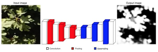
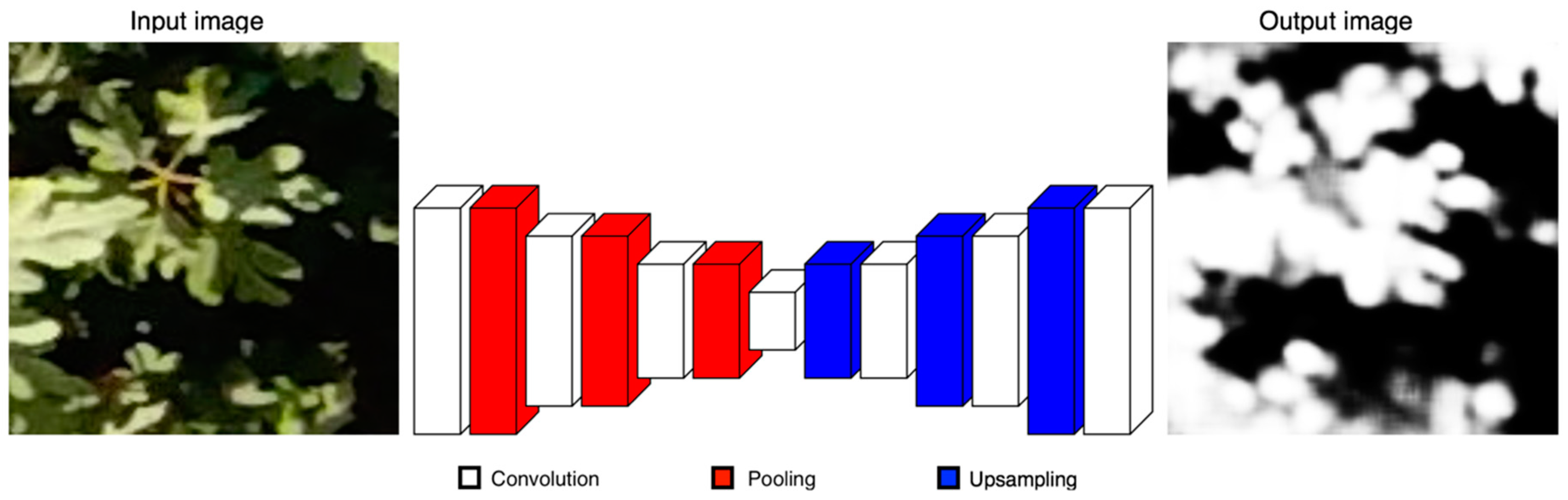
Our CNN is inspired by SegNet architecture [14], which uses the principles of an encoder-decoder architecture to perform pixel-wise semantic segmentation. Unlike SegNet, our architecture comprises only 7 learnable layers as follows. The encoder section has 4 convolutional layers and 3 pooling layers to generate a low-resolution representation. The decoder part has 3 convolutional layers and 3 upsampling layers for producing pixel-wise predictions. In Figure 3 we present a scheme of our approach. We use fewer convolutional layers and have a smaller number of trainable parameters than SegNet-Basic, the smaller version of SegNet, turning it into a simpler model. Likewise, we discard the multi-class soft-max classifier as a final layer because we expect only 2 classes. On the contrary, a sigmoid layer is used in the output to predict a probability of that each pixel belongs to one class or another.

The input of our CNN is a 128 × 128 RGB patch and the output is a 128 × 128 greyscale patch; details about image sizes are presented in the next section. For training, firstly each pixel value is normalized to a range of 0 to 1. The patch is passed through a set of different convolutional layers, where we use relatively large receptive fields (7 × 7) for the first layer and very small receptive fields (3 × 3) for the rest. The convolution stride is fixed to 1 pixel and a zero-padding option is used for all layers. Two activation functions are used. A Sigmoid activation is applied after the last convolution layer and for the rest, a Rectified Linear Unit (ReLU) activation is employed in order to introduce nonlinearities. Maxpooling is done over 2 × 2 windows with stride 2. Upsampling is performed by a factor of 2 × 2 to increase the resolution of the image. In

Table 2. Summary of the CNN configuration. First column indicates the size of the filters while second column details the output of the layer.

Details of Our CNN
Input (128 × 128 × 3 image)
[7 × 7]	[32] [128 × 128]
pooling
[3 × 3]	[8] [64 × 64]
pooling
[3 × 3]	[8] [32 × 32]
pooling
[3 × 3]	[8] [16 × 16]
upsampling
[3 × 3]	[8] [32 × 32]
upsampling
[3 × 3]	[16] [64 × 64]
upsampling
[3 × 3]	[1] [128 × 128]
Output (128 × 128 × 1 image)

we present a summary of our proposed CNN architecture. The convolutional layers parameters are denoted as “[receptive field size] |{layer output} = [number of channels] [image size].”

The best set of hyperparameters that define the structure of the network (e.g., number of layers, number and size of filters) was determined by experience and performing a series of experiments. Concretely, we choose the following parameters: epochs = 120, batch size = 32, loss function = Binary cross-entropy, optimizer = Adadelta and initial learning rate = 1.0.

Our CNN is developed in Python using Keras [31] and TensorFlow [32] libraries. The experiments are performed on a laptop with a Linux platform, a processor Intel^® Core™ i7-8750H CPU @ 2.20GHz x 12, 16 GB RAM and NVIDIA GPU GeForce GTX 1070. We convert the final decoder output to a binary image in order to compute the metrics for evaluation by way of a simplest thresholding method. Values below 0.5 are turned to zero and all values above that threshold to 1.

4.2. Input Data Preparation

In our proposed data set, there are only 10 labelled images of 2000 × 1500 pixels. However, a fig leaf in these images is represented, on average, by a region of 25 × 25 pixels. Therefore, they contain a large number of leaves samples subjected to different conditions, with which it is possible to carry out training of our CNN without the need to resort to data augmentation techniques. We perform in each labelled image a sampling of overlapping patches with a fixed stride. The image is divided into patches of 128 × 128 pixels with horizontal and vertical overlapping between regions of 70% (90 pixels), generating more input data. We observe that as the size of the patch increases, the performance improves. Nevertheless, larger patches involve more processing time and the problem of getting a small number of patches per image. Finally, we work with a total of 19,380 patches with their respective GT.

5. Experimental Results

In this section, we evaluate the proposed approach in a comprehensive way. We carry out tests with the smaller version of SegNet, SegNet-Basic. SegNet is specially designed to perform road scene segmentations, a multi-class segmentation problem, therefore it has a complex architecture that needs more computing resources than we have in order to deal with the large number of trainable parameters. However, the experiments are designed to demonstrate the accuracy in fig crop segmentation despite all the challenges present in the proposed data set.

5.1. Evaluation Measures

We used measures based on True Positives (TP), False Positives (FP), False Negatives (FN) and True Negatives (TN) to determine the performance of our CNN. The measures are Accuracy, Specificity, Precision, Recall, Negative Predictive Value (NPV) and F-measure [33]. The equations are presented in

Table 3. Evaluation metrics.

Metric	Formula
Accuracy	$\left(\mathrm{TP}+\mathrm{TN}\right)/\left(\mathrm{TP}+\mathrm{TN}+\mathrm{FP}+\mathrm{FN}\right)$
Specificity	$\mathrm{TN}/\left(\mathrm{TN}+\mathrm{FP}\right)$
Precision	$\mathrm{TP}/\left(\mathrm{TP}+\mathrm{FP}\right)$
Recall	$\mathrm{TP}/\left(\mathrm{TP}+\mathrm{FN}\right)$
NPV	$\mathrm{TN}/\left(\mathrm{TN}+\mathrm{FN}\right)$
F-measure	$\left(2\ast \mathrm{TP}\right)/\left(2\ast \mathrm{TP}+\mathrm{FN}+\mathrm{FP}\right)$

, where: TP are the fig plant pixels correctly classified, FP are pixels proposed as fig plant pixels but these do not really correspond to some part of the bushes, FN are fig plant pixels contained in the GT which are not detected by the system and TN are non-plant pixels properly classified.

5.2. Colour Vegetation Indices Performance

The colour index-based methods have been widely used in the state-of-the-art of vegetation detection due to their low computational cost and comparable performance to more complex algorithms [34]. First, we evaluate the performance of these indices to use them as baseline in further comparisons. The following colour indices are assessed: Normalized Difference Index (NDI), Excess Green Index (ExG), Excess Red Index (ExR), Colour Index of Vegetation Extraction (CIVE), Excess Green minus Excess Red Index (ExGR), Vegetative Index (VEG), Combined Indices 1 (COM1), Modified Excess Green Index (MExG), Combined Indices 2 (COM2) and Green minus Blue (GB). For details, see Reference [34] and

Table 4. Colour vegetation indices formulas.

Index	Formula
NDI	$128\ast \left(\left(\left(\mathrm{G}-\mathrm{R}\right)/\left(\mathrm{G}+\mathrm{R}\right)\right)+1\right)$
ExG	$2\ast \mathrm{G}-\mathrm{R}-\mathrm{B}$
ExR	$1.3\ast \mathrm{R}-\mathrm{G}$
CIVE	$0.441\ast \mathrm{R}-0.811\ast \mathrm{G}+0.385\ast \mathrm{B}+18.78745$
ExGR	$\mathrm{ExG}-\mathrm{ExR}$
VEG	$\mathrm{G}/({\mathrm{R}}^{\mathrm{a}}{\ast \mathrm{B}}^{\left(1-\mathrm{a}\right)})$$,\mathrm{a}=0.667$
COM1	$\mathrm{ExG}+\mathrm{CIVE}+\mathrm{ExGR}+\mathrm{VEG}$
MExG	$1.262\ast \mathrm{G}-0.884\ast \mathrm{R}-0.311\ast \mathrm{B}$
COM2	$0.36\ast \mathrm{ExG}+0.47\ast \mathrm{CIVE}+0.17\ast \mathrm{VEG}$
GB	$\mathrm{G}-\mathrm{B}$

.

In order to obtain Precision-Recall (PR) plots and Receiver Operating Characteristic (ROC) curves, we varied the threshold to classify the pixels into crop and non-crop classes after calculating the vegetation indices in three images of the proposed data set which belong to different areas of the crop, see Figure 4. The first row of Figure 5 illustrates the PR plots. In general, CIVE, COM2, ExG and MExG indices have a good performance. With the use of the ROC analysis for these indices (see second row of Figure 5), MExG demonstrate a larger area under the curve compared to the rest, indicating a superior performance to detect vegetation. Using an adequate threshold, MExG achieves the following recall rates: 89.63% for image 10_A, 93.91% for image 75_A and 89.02% for image 98_A, with a precision of 64% for the first image, 96% for the second image and 92% for the third. Although the images were collected at the same time of day, the fig plants in image 98_A have a different visual appearance due to the position that the camera had with respect to the sun when the image was captured.

Table 5. Performance evaluation on our data set.

Index	Accuracy (%)
	Mean	σ	Min	Max
CIVE	85.53	5.22	73.40	91.17
ExG	85.93	6.22	71.70	91.84
COM2	86.20	7.21	69.52	93.13
MExG	88.31	4.84	76.95	92.09

gives a comparison of fig plant detection results using the best vegetation indexes in ten images of our data set. The Otsu thresholding algorithm [35] is used with the aim to obtain green pixels after applying the vegetation indices. MExG obtains the maximum mean accuracy value. All vegetation indexes fail to detect the leaves located in the lower parts of the bushes, which present a dark tone. Likewise, the performance is very bad when the image contains many areas with green weed.

5.3. Convolutional Neural Network Performance

To evaluate the performance of the network, we divide the dataset into an 80–20% split for training and test images. Figure 6 depicts the loss and accuracy for training and test sets over 400 epochs, where an epoch is considered as an iteration over all the training or test set. The curves show that the amount of data to train the model is adequate. The model has a low overfitting and a good generalization. For the following results, we decided to stop the training in 120 epochs because later the test loss starts increasing in a clearer way.

Table 6. Performance of crop segmentation in Test set.

Metric	(%)
	Our Proposal	SegNet-Basic
Accuracy	93.84	93.82
Specificity	92.79	94.33
Precision	92.00	93.49
Recall	95.05	93.22
NPV	95.55	94.10
F-measure	93.50	93.35

shows the experimental results obtained from the test set with our proposal and SegNet-Basic. The available implementation of SegNet-Basic based on the Caffe library [36] was used. We set the following parameters: batch size = 32, iterations = 30,070 (62 epochs), weight delay rate = 0.0005, learning rate = 0.1 and Stochastic Gradient Descent solver for optimization. We achieve the same performance as SegNet-Basic in segmenting fig plants but with a considerable reduction in training time. The model training time is decreased due to the diminished number of trainable parameters (0.010M vs. 1.425M of SegNet-Basic). The training time of our model, for 120 epochs with 15K images, took approximately 45 min, while SegNet-Basic, trained for 62 epochs with the same pool of training images, took about 3 h. We achieve an accuracy of 93.84% with 3.84% of FP and 2.30% of FN. Likewise, an F-measure of 93.50%, which represents the harmonic mean of recall and precision.

We test our trained model with patches of different sizes in order to demonstrate that the performance of the network is maintained. The configurations are the following: 32 × 32 pixels without overlapping (2961 patches), 64 × 64 pixels with an overlapping of 25 pixels (1938 patches) and 256 × 256 pixels with an overlapping of 220 pixels (1800 patches). Different overlap sizes are used to maintain approximately the same number of patches.

Table 7. Performance of crop segmentation with patches of different sizes.

Metric	Patch Sizes
	32 × 32	64 × 64	256 × 256
Accuracy	89.55	90.25	90.92
Specificity	83.04	83.00	84.73
Precision	81.99	83.00	84.25
Recall	97.69	97.89	98.12
NPV	97.29	97.52	97.79
F-measure	88.93	89.70	90.57

shows the metrics obtained for each of the options. In the three cases, an accuracy greater than 89% is achieved even though the model was trained with patches of 128 × 128 pixels.

Figure 7 shows the activation maps of our network for a test patch. Only the most illustrative activation map of each convolutional layer is shown. The images visualize the internal operations to carry out a low-level representation of the fig plant and then perform its reconstruction. Red regions represent strong activations. Likewise, the pixel-wise probability map and the GT image are presented. Examples of qualitative results are shown in Figure 8. Each column displays a patch used to testing. First row presents the RGB data, the second column contains the GT and the third column displays the probability output. These results show that the trained network can deal with the shadows and the specular reflections that occur on the leaves. In addition, the CNN is capable of correctly exclude different types of soil, camouflaged plants, dry grass and narrow-leaf grass.

In Figure 9, we show some challenges for semantic segmentation of crops. The first four columns show cases of broad-leaf weeds. The appearance of these weeds is very similar to the fig leaves. In fact, using only the images as reference, it was difficult for the experts to decide if those plants belonged to small fig plants or not. The following column presents a problem caused by a bucket, which is used by farmers as a work tool. The last column displays a patch with dry plants of a contiguous maize crop. This situation occurs when the UAV flies over the edges of the interest field. Although all these cases are scarce, it is important to consider them in order to build robust plant detection systems that can work under less restrictive circumstances.

To analyse the effect of performance with different samples for training, we perform a cross-validation experiment with different training and test set pairs. We split our patches many times into two parts of 80% for training and 20% for testing, with which we can generate a total of 45 possible combinations. The results of the cross-validation are shown in Figure 10. An accuracy greater than 89.28% is obtained in all cases, which is an excellent performance considering the complexity of the data. We achieve a mean accuracy of 93.85% with a standard deviation of 1.27%. The lowest accuracy is reached when the test patches are extracted from the images 10_A and 101_A, see Figure 11. These images contain regions of fig plants that delimit the cultivated land and regions that belong to other crops or roads. The other images that were used for training do not present these conditions because they were captured inside the crop area. The use of more labelled images might help to avoid all these difficulties.

To evaluate the segmentation performance in each of the whole images, all the predicted outputs of a complete image are integrated into single probability matrix of size 2000 × 1500. Each prediction value of the patch is stored in the corresponding cell of the matrix. If a cell contains several prediction values dues to the overlap that exists among the patches, then these values are averaged. The final probability matrix is binarized to compute the evaluation metrics, where values below 0.5 are turned to zero and otherwise to 1. This process is carried out in each of the cross-validation experiments, so it is possible to get 9 probability matrices for each labelled image.

Table 8. Accuracy, precision and recall of whole images.

Image	Accuracy (%)				Precision (%)				Recall (%)
	Mean	σ	Min	Max	Mean	σ	Min	Max	Mean	σ	Min	Max
10_A	93.01	2.99	85.40	94.88	86.15	5.89	71.64	90.40	96.63	0.96	95.12	98.13
10_B	94.87	0.63	93.27	95.37	96.57	0.77	95.12	97.75	96.61	1.45	93.17	97.96
18_A	93.52	0.63	92.15	94.09	91.39	1.40	88.64	93.03	98.15	0.70	97.06	99.25
36_A	94.42	0.23	93.92	94.72	94.55	0.94	93.19	95.97	96.94	1.25	94.53	98.40
43_A	95.47	0.35	94.53	95.69	95.91	1.10	93.43	96.96	97.37	0.81	96.40	98.73
51_A	92.94	0.46	91.88	93.28	92.84	1.65	89.54	94.65	94.75	1.55	92.11	96.80
75_A	94.77	0.28	94.40	95.10	96.78	0.90	94.51	97.46	95.64	1.00	94.51	97.58
83_A	95.27	0.43	94.17	95.56	95.50	1.51	91.82	96.75	96.51	1.19	94.86	98.84
98_A	90.54	1.47	88.50	92.69	97.03	0.77	95.58	97.72	84.96	3.51	80.48	90.47
101_A	96.10	0.90	93.72	96.71	93.64	3.49	85.66	96.65	95.13	2.43	92.03	97.78

shows the mean, the standard deviation and the minimum and maximum of the accuracy, precision and recall percentages for all labelled images. The smallest percentages of accuracy and precision are obtained in 10_A image when it is joined with 101_A image to be used as test data (as described above). A mean accuracy greater than 90.54 is obtained in all images, so we demonstrate that the good performance is kept after the integration of all prediction patches of an image. Although our model performs well, more samples of crop and non-crop classes are necessary to achieve a robust system, so therefore the capacity of the network would have to be modified to deal with the new problems. The proposed CNN was trained to specifically segment fig plants. However, under adequate training, the proposed method is applicable to other datasets of similar nature. The resolution of the image could generate a different performance in the segmentation process. The low-resolution images do not contain all the details of the leaves that are captured in a high-resolution image. All this should be evaluated in future work.

6. Conclusions

We have proposed a fig plant segmentation method based on deep learning and a challenging data set with its ground truth labelled by hand at the pixel level. The data set is of particular interest to smart farming and computer vision researchers. It consists of 110 high resolution aerial images captured by an UAV. Images show an open field fig crop, where there is a great variability in tones and shapes of the leaves due to the plant morphology and the different positions of the camera relative to the sun when the image was captured. In addition, the background is really complex because it can contain several elements which increase the difficulty of the plant detection process. The fig species is Ficus carica, whose bushes are tall and whose life cycle is long, so the use of aerial robots is more appropriate than terrestrial ones for their monitoring.

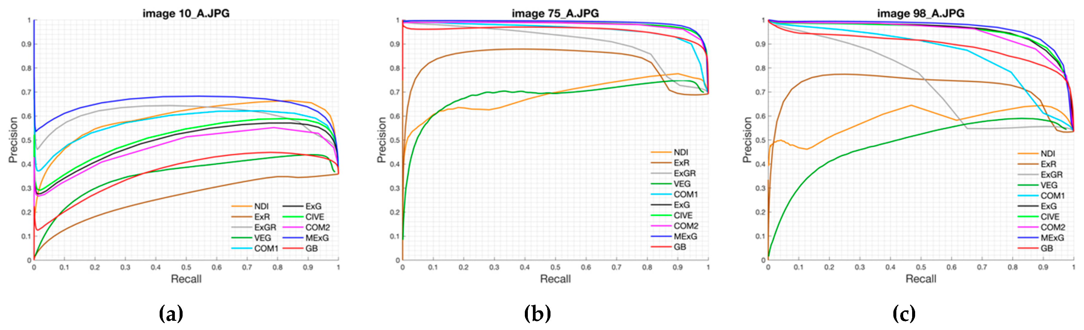
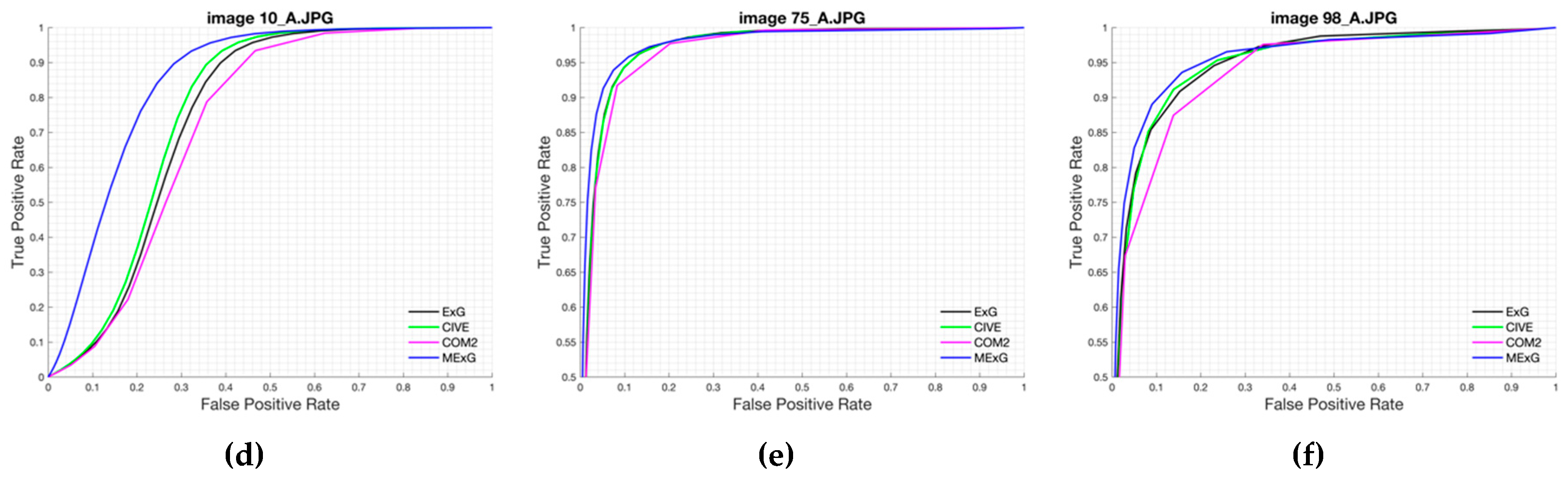
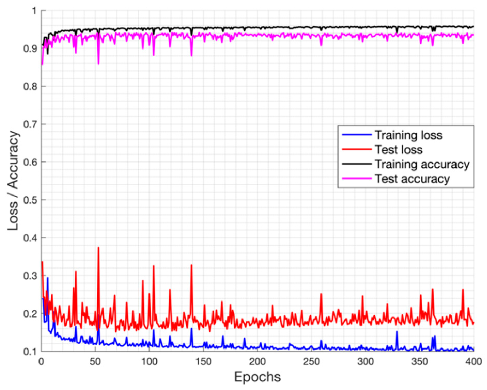
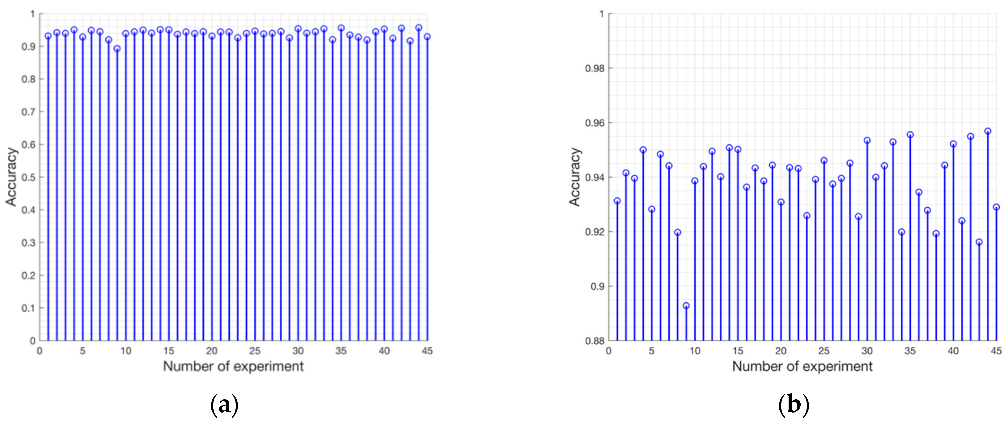
Our approach was based on a CNN model with an encoder-decoder architecture trained end-to-end. The experimental results showed that our model can be trained in just 45 min while maintaining its ability to accurately segment the fig plants. The CNN-based method is adequate to deal with the two-class segmentation problem, even in highly challenging scenarios such as the segmentation of fig plants introduced in this work. The encoder-decoder architecture is capable to learn the discriminative filters that help detect fig foliage in order to segment them from the background. On the other hand, the evaluation of vegetation indices showed that ExG, CIVE, COM2 and MExG have an acceptable performance in our data, although it is clearly surpassed by the proposed convolutional encoder-decoder architecture. These indices can be used as first stage where it is necessary to isolate the vegetation as the object of interest quickly in order to do tasks of a higher level such as recognition or classification of plants. Future work is aimed at optimizing the model to improve results and consider other cases of fig crops in different seasons. Likewise, we plan to carry out experiments in orthomosaic images generated from our fig images. Orthomosaics are of great importance in agriculture because they offer more information, which could be used to analyse the conditions of the field.

References

1. Haug, S.; Ostermann, J. A crop/weed field image dataset for the evaluation of computer vision based precision agricultural tasks. In European Conference on Computer Vision; Springer: Cham, Switzerland, 2015; pp. 105–116. [Google Scholar]
2. Hernández-Hernández, J.L.; García-Mateos, G.; González-Esquiva, J.M.; Escarabajal-Henarejos, D.; Ruiz-Canales, V.; Molina-Martínez, J.M. Optimal color space selection method for plant/soil segmentation in agriculture. Comput. Electron. Agric. 2016, 122, 124–132. [Google Scholar] [CrossRef]
3. Chebrolu, N.; Lottes, P.; Schaefer, A.; Winterhalter, V.; Burgard, W.; Stachniss, C. Agricultural robot dataset for plant classification, localization and mapping on sugar beet fields. Int. J. Robot. Res. 2017, 36, 1045–1052. [Google Scholar] [CrossRef]
4. Cowart, N.; Graham, J. Within-and among-individual variation in fluctuating asymmetry of leaves in the fig (Ficus carica L.). Int. J. Plant Sci. 1999, 160, 116–121. [Google Scholar] [CrossRef]
5. Barolo, M.I.; Mostacero, N.R.; López, S.N. Ficus carica L. (Moraceae): An ancient source of food and health. Food Chem. 2014, 164, 119–127. [Google Scholar] [CrossRef]
6. FAOSTAT. Food and Agriculture Organization of the United Nations. 2016. Available online: http://www.fao.org/faostat/en/#data/QC/visualize (accessed on 15 January 2019).
7. SIAP. Sistema de Información Agrolimentaria y Pesquera. 2015. Available online: http://infosiap.siap.gob.mx/aagricola_siap_gb/icultivo/index.jsp (accessed on 31 March 2019).
8. Zhang, C.; Kovacs, V. The application of small unmanned aerial systems for precision agriculture: a review. Precis. Agric. 2012, 13, 693–712. [Google Scholar] [CrossRef]
9. Berni, J.; Zarco-Tejada, P.; Suárez, L.; Fereres, E. Thermal and narrowband multispectral remote sensing for vegetation monitoring from an unmanned aerial vehicle. IEEE Trans. Geosci. Remote Sens. 2009, 47, 722–738. [Google Scholar] [CrossRef]
10. Sa, I.; Chen, Z.; Popović, M.; Khanna, R.; Liebisch, F.; Nieto, J.; Siegwart, R. WeedNet: Dense semantic weed classification using multispectral images and MAV for smart farming. IEEE Robot. Autom. Lett. 2018, 3, 588–595. [Google Scholar] [CrossRef]
11. Goodfellow, I.; Bengio, Y.; Courville, A. Deep Learning; MIT Press: Cambridge, MA, USA, 2016. [Google Scholar]
12. LeCun, Y.; Bengio, Y.; Hinton, G. Deep learning. Nature 2015, 521, 436–444. [Google Scholar] [CrossRef]
13. Long, J.; Shelhamer, E.; Darrell, T. Fully convolutional networks for semantic segmentation. In Proceedings of the 2015 IEEE Conference on Computer Vision and Pattern Recognition (CVPR), Boston, MA, USA, 7–12 June 2015. [Google Scholar]
14. Badrinarayanan, V.; Kendall, A.; Cipolla, R. Segnet: A deep convolutional encoder-decoder architecture for image segmentation. IEEE Trans. Pattern Anal. Mach. Intell. 2017, 39, 2481–2495. [Google Scholar] [CrossRef]
15. Kamilaris, A.; Prenafeta-Boldú, F.X. A review of the use of convolutional neural networks in agriculture. J. Agric. Sci. 2018, 156, 312–322. [Google Scholar] [CrossRef]
16. Chen, L.C.; Papandreou, G.; Kokkinos, I.; Murphy, K.; Yuille, A.L. Deeplab: Semantic image segmentation with deep convolutional nets, atrous convolution and fully connected crfs. IEEE Trans. Pattern Anal. Mach. Intell. 2017, 40, 834–848. [Google Scholar] [CrossRef] [PubMed]
17. Kamilaris, A.; Prenafeta-Boldú, F.X. Deep learning in agriculture: A survey. Comput. Electron. Agric. 2018, 147, 70–90. [Google Scholar] [CrossRef]
18. Ye, M.; Cao, Z.; Yu, Z.; Bai, X. Crop feature extraction from images with probabilistic superpixel markov random field. Comput. Electron. Agric. 2015, 114, 247–260. [Google Scholar] [CrossRef]
19. Li, Y.; Cao, Z.; Lu, H.; Xiao, Y.; Zhu, Y.; Cremers, A.B. In-field cotton detection via region-based semantic image segmentation. Comput. Electron. Agric. 2016, 127, 475–486. [Google Scholar] [CrossRef]
20. Milioto, A.; Lottes, P.; Stachniss, C. Real-time semantic segmentation of crop and weed for precision agriculture robots leveraging background knowledge in CNNs. In Proceedings of the IEEE International Conference on Robotics and Automation 2018 (ICRA 2018), Brisbane, Australia, 21–25 May 2018. [Google Scholar]
21. Linnaeus, C. Species Plantarum; Impensis GC Nauk: Berlin, Germany, 1753. [Google Scholar]
22. Lottes, P.; Behley, J.; Milioto, A.; Stachniss, C. Fully convolutional networks with sequential information for robust crop and weed detection in precision farming. IEEE Robot. Autom. Lett. 2018, 3, 2870–2877. [Google Scholar] [CrossRef]
23. Liu, J.; Pattey, E. Retrieval of leaf area index from top-of-canopy digital photography over agricultural crops. Agric. For. Meteorol. 2010, 150, 1485–1490. [Google Scholar] [CrossRef]
24. Burgos-Artizzu, X.P.; Ribeiro, A.; Guijarro, M.; Pajares, G. Real-time image processing for crop/weed discrimination in maize fields. Comput. Electron. Agric. 2011, 75, 337–346. [Google Scholar] [CrossRef] [Green Version]
25. Hamuda, E.; Mc Ginley, B.; Glavin, M.; Jones, E. Automatic crop detection under field conditions using the HSV colour space and morphological operations. Comput. Electron. Agric. 2017, 133, 97–107. [Google Scholar] [CrossRef]
26. Ha, J.G.; Moon, H.; Kwak, J.T.; Hassan, S.I.; Dang, L.; Lee, O.N.; Park, H.Y. Deep convolutional neural network for classifying fusarium wilt of radish from unmanned aerial vehicles. J. Appl. Remote Sens. 2017, 11, 042621. [Google Scholar] [CrossRef]
27. Dang, L.M.; Hassan, S.I.; Suhyeon, I.; Sangaiah, A.K.; Mehmood, I.; Rho, S.; Seo, S.; Moon, H. UAV based wilt detection system via convolutional neural networks. Sustain. Comput. Inf. Syst. 2018. [Google Scholar] [CrossRef]
28. Di Cicco, M.; Potena, C.; Grisetti, G.; Pretto, A. Automatic model based dataset generation for fast and accurate crop and weeds detection. In Proceedings of the 2017 IEEE/RSJ International Conference on Intelligent Robots and Systems (IROS), Vancouver, Canada, 24–28 September 2017. [Google Scholar]
29. DroneDeploy. Work Smarter with Drone Data. 2018. Available online: https://www.dronedeploy.com (accessed on 31 March 2019).
30. ImageAnnotation. Image Annotation Tool with Image Masks. 2010. Available online: https://lear.inrialpes.fr/people/klaeser/software_image_annotation (accessed on 23 September 2018).
31. Keras. The Python Deep Learning Library. François Chollet and Others. 2015. Available online: https://keras.io (accessed on 31 March 2019).
32. TensorFlow. Large-Scale Machine Learning on Heterogeneous Systems. 2015. Available online: https://www.tensorflow.org (accessed on 31 March 2019).
33. Labatut, V.; Cherifi, H. Accuracy measures for the comparison of classifiers. In Proceedings of the 5th International Conference on Information Technology, Amman, Jordan, 11–13 May 2011. [Google Scholar]
34. Hamuda, E.; Glavin, M.; Jones, E. A survey of image processing techniques for plant extraction and segmentation in the field. Comput. Electron. Agric. 2016, 125, 184–199. [Google Scholar] [CrossRef]
35. Otsu, N. A threshold selection method from gray-level histograms. IEEE Trans. Syst. Man Cybern. 1979, 9, 62–66. [Google Scholar] [CrossRef]
36. Caffe SegNet. Implementation of SegNet: A Deep Convolutional Encoder-Decoder Architecture for Semantic Pixel-Wise Labelling. 2016. Available online: https://github.com/alexgkendall/caffe-segnet (accessed on 2 May 2019).
Figure 1. (a) Ground view and (b) top-view of fig shrubs.
Remotesensing 11 01157 g001
Figure 2. Views of image regions manually labelled: (a) Labelled image segment (400 × 200 pixels), the labelled pixels are represented in red colour; (b) and (c) Zoom view of a small region (112 × 112 pixels) which shows the level of detail of the labelling process.
Remotesensing 11 01157 g002
Figure 3. A scheme of the proposed architecture.
Remotesensing 11 01157 g003
Figure 4. Images of 2000 × 1500 pixels used to evaluate the performance of colour vegetation indices: (a) image 10_A; (b) image 75_A and (c) image 98_A.
Remotesensing 11 01157 g004
Figure 5. PR plots (first row) and ROC curves (second row) for three images of the proposed data. Performance evaluated on the images: (a) and (d) 10_A; (b) and (e) 75_A; and (c) and (f) 98_A.
Remotesensing 11 01157 g005aRemotesensing 11 01157 g005b
Figure 6. Loss and accuracy of training and test.
Remotesensing 11 01157 g006
Figure 7. Visualization of the activations of our network: (a) input image. The output maps of the encoder part from: (b) the 128 × 128 convolutional+ReLU layer; (c) the 64 × 64 convolutional+ReLU layer; (d) the 32 × 32 convolutional+ReLU layer; and (e) the 16 × 16 convolutional+ReLU layer. The output maps of the decoder: (f) the 32 × 32 convolutional+ReLU layer; (g) the 64 × 64 convolutional+ReLU layer; (h) the 128 × 128 convolutional+Sigmoid layer; and (i) the output and (j) GT image.
Remotesensing 11 01157 g007
Figure 8. Qualitative results of six test patches: RGB image input (first row), GT (second row) and Predictions (third row).
Remotesensing 11 01157 g008
Figure 9. Some problems identified: RGB image inputs (first row), GT (second row) and Predictions (third row).
Remotesensing 11 01157 g009
Figure 10. Accuracy values obtained with distinct training and validation set pairs. (a) and (b) graphs represent the same data. In (b) graph the y-axis limits are different only for better visualization.
Remotesensing 11 01157 g010
Figure 11. Images used to extract the test patches in the case where the lowest accuracy was obtained: (a) image 10_A and (b) image 101_A.
Remotesensing 11 01157 g011