Article

Three-Level NPC Inverter Incipient Fault Detection and Classification using Output Current Statistical Analysis

1
Laboratoire IRECOM, University Djillali Liabès, 22000 Sidi Bel Abbes, Algeria
2
GeePs, UMR 8507, CNRS, CentraleSupélec, Univ. Paris Sud, Université Paris Saclay, Sorbonne Univ, 75006 Paris, France
3
L2S, UMR 8506, CNRS, CentraleSupélec, Univ. Paris Sud, Université Paris Saclay, 91190 Saint-Aubin, France
4
Shanghai Maritime University, Department of Electrical Automation, Shanghai 201306, China
5
Faculty of Computer Engineering and Media, De Montfort University, Leicester LE1 9BH, UK
*
Author to whom correspondence should be addressed.
Energies 2019, 12(7), 1372; https://doi.org/10.3390/en12071372
Submission received: 20 March 2019 / Revised: 2 April 2019 / Accepted: 2 April 2019 / Published: 9 April 2019
(This article belongs to the Special Issue Fault Diagnosis and Fault-Tolerant Control)

Abstract

:
This paper deals with open switch Fault Detection and Diagnosis (FDD) in three-level Neutral Point Clamped (NPC) inverter for electrical drives. The approach is based on the already available phase current time series measurements for different operating conditions (motor speed, load, and environment noise). Both fault detection and classification are studied and the efficiency performances of the proposed selected features are shown. For the fault detection, we focus on the first four statistical moments and the extracted features and then the Cumulative Sum (CUSUM) algorithm as the feature analysis technique to improve the performances. For the classification study, we propose to couple the knowledge on the faulty system brought by the statistical moments and the Kullback-Leibler divergence particularly suitable for the detection of incipient changes. The Principal Component Analysis (PCA) is then used to perform the classification. A 2D framework is obtained, which allows the faults to be classified efficiently within the considered operating conditions for all the selected fault durations.

1. Introduction

In recent decades, more and more applications in industrial, manufacturing, or the transportation domain have been increasingly electrified for efficiency and environmental issues [1,2,3]. However, due to the reliability, availability, and maintainability requirements [4], the system must remain operational despite fault occurrence and its performances must remain robust to environmental nuisances. Therefore, effort is put toward the design and health monitoring of the electrical drives. Beside electrical machines, voltage source inverters are one of the most sensitive components prone to faults or failures [5].
During the last several years, multilevel inverters have become increasingly popular. Among their good properties, one can mention their output voltage quality, their improvement, and the reduction of the electrical constraints on the power switches as well as the reduction of the switching frequency [6,7]. Such inverters generate less electromagnetic perturbations, and, therefore, the size and the cost of their main filter can be reduced [8]. As an example, in Reference [8], the authors have made a comparison between four topologies of inverters in terms of semiconductor and capacitors losses including the conventional structure, an interleaved two-level inverter, the Neutral Point Clamped (NPC) structure, and the cascaded three-level H-bridge. The NPC inverter [9] has proved to be the most efficient. However, compared to the classical 2-level inverter, the main drawbacks of the multilevel inverters are the higher number of components (power switches and capacitors) and a more complex control [10].
In this paper, we have chosen the three-level NPC inverter since it has lower inverter losses, and lower stress on the power switches at higher switching frequencies when compared to a two-level inverter for electric vehicle applications [10].
In industrial applications using variable-speed AC drives, different studies have proved that about 38% of the faults are due to failures in the power device [11]. These faults can be classified in three classes shown below.
  • Abrupt faults that suddenly occur, inducing significant changes in the system behavior.
  • Gradual faults. These fault types can be considered as a slight but abnormal increasing over time variation in parameters and/or variables of the process.
  • Intermittent faults. The immediate effect can be negligible but its repetition may lead to failures.
Abrupt fault detection and their effects on electrical machines have been widely studied during the last decade [12]. For gradual fault, it is crucial to detect it at its earliest stage or at its smallest detectable severity. At this stage, the fault is considered as incipient and is becoming a hot topic in academic research [13]. Intermittent fault is the most difficult one to detect because it occurs randomly with different durations and its severity can also vary from incipient to severe.
In this study, we focus on the detection of intermittent faults, which affects the power switches of a three-level NPC inverter feeding a speed controlled induction machine drive.
Recently, several methods have been investigated for evaluating fault occurrence in power converters [14,15,16]. Some efficient detection methods are based on the evaluation of the electrical components in the Park’s transform domain [17]. Unfortunately, in these works, authors have addressed the detection of abrupt fault with a high severity level. They have not addressed the issue of incipient faults defined as faults with a severity level equal or lower than the environmental noise. This is the case of the slowly developing fault at its very early stage. In our study, we propose analysing the available time domain phase current measurements in the natural frame to detect and classify power converter faults in a speed control induction motor drive.
This paper is organized as follows. In Section 2, the drive under consideration is described and its main characteristics are presented. The studied faults and their effects on the phase currents temporal series are introduced. Section 3 introduces the fault Detection and Diagnosis methodology. In Section 4, the fault detection methodology with its different steps is applied and the results are derived. The fault detection performances for incipient faults are computed in different operating conditions (speed, load, torque, and noise). In Section 5, a classification based on the fault severity is proposed. The influence of the operating conditions is highlighted. Section 6 concludes the paper.

2. Induction Machine Drive and Fault Description

2.1. Description of the Induction Machine Drive

The Induction Machine (IM) drive is displayed in Figure 1. It includes an outer speed loop and two inner current loops in the (d,q) synchronous rotating frame. The induction machine is fed with a three-level Neutral Point Clamped (NPC) inverter. Its structure is detailed in Figure 2 [8]. The inverter is composed of three legs (A, B, and C) with four active switches and anti-parallel diodes for each leg. The DC bus has two capacitors, which provides the middle point “O”. The NPC inverter is used for generating the three voltages (va, vb, and vc) applied across the windings of the induction machine. In the following, with no loss of generality, the NPC inverter is switched at 10 kHz. The sampling frequency is set at 100 kHz.
The main characteristics of the drive are summarized in Table 1.

2.2. Fault Impact on Electrical Signals

In the literature, the main faults that occurred on power switches are:
  • Short-Circuit Faults (SCF) that can lead to brutal damages on the switch itself or even on the drive. These faults usually cause the tripping of fuses and, in tolerant structures (conservative design), the turn-on of spare power switches.
  • Open-Switch Faults (OSF) that have less immediate negative effect. However, the cumulative effect may lead to non-reversible degradations.
Therefore, in the following, we assume that one of the NPC power switches suffers from misfiring, which leads to an open circuit fault in the leg. Despite the closed loop control, there will be a fault effect. The NPC output currents flowing into the machine windings will carry information on the fault occurrence. They are denoted as iSA, iSB, and iSC, which can be seen in Figure 1. They will be analyzed as fault signatures by the fault detection and diagnosis methodology.
As an example, Figure 3 shows the current in phase A when a permanent OSF is introduced at 100 ms. Thanks to the speed and current regulators, less than 12 ms after fault occurrence, the fault effect is almost erased. However, if the fault is repetitive (due to aging or thermal stress), it will increase the fatigue of the power converter and may induce cascaded faults or failures. Moreover, each transient increases the amount of energy absorbed from the power supply.
If the fault duration is very short, the fault effect is less and its detection becomes more tedious. Figure 4 displays the case of an OSF of 500 µs. The fault starts at 100 ms.
Therefore, to prevent unwanted stops and poor performances, monitoring of the power converter to diagnose such fault is mandatory.
In the following, we will focus our study on these OSF with a short duration (higher or equal to the switching period). The FDD methodology will be evaluated for different operating points and in different noise conditions.

2.3. Fault Description and Operating Conditions

In our work, all the short durations OSF are evaluated by assuming that each fault occurrence is in one electrical period of the current signal. The fault length will never be larger than the signal period nor lower than the switching frequency period. To evaluate the effect of the fault on the system, several operating conditions are considered.
First, the faults’ severities are classified according to their durations. In the following, 10 cases under study are considered from 100 μs to 1 ms with 100 µs step (100 μs, 200 μs, …, 900 μs, 1 ms). The smallest fault duration value is related to the NPC switching frequency set at 10 kHz.
For the analyses of the 10 faulty cases, several operating points are considered for the drive.
  • Three rotating speeds (20, 40, and 60 rad/s) according to the European Urban Driving Cycle (EUDC).
  • Three different loads (no load, 50% and 100% of the rated torque).
Additionally, five Signal to Noise Ratio (SNR) (20 dB, 25 dB, 30 dB, 35 dB, and 40 dB) corresponding to different noise levels are considered to evaluate the influence of the environmental nuisances on the fault diagnosis.
In this paper, only a selection of the results obtained will be presented. The selected ones better highlight the fault detection and classification performances for different noises, speeds, and load conditions. The most severe conditions (OSF with lowest duration, lowest SNR, lowest speed, and highest load) are often chosen to highlight the main difficulties for efficient fault detection and diagnosis.

3. Fault Evaluation Process

3.1. Proposed Methodology

We propose a fault detection methodology that can be described in four main steps.
  • The first step is the Modeling. In this step, a model describing the behavior of the system is derived. This model can be analytical (i.e., using physical laws describing the system), linguistic (i.e., using a linguistic description of the system), or data driven (i.e., using data history from the system). In the proposed work, a data driven-based approach is considered. The drive is simulated for different conditions of noise, OSF durations, and operating points (load and speed).
  • The second step is the pre-processing. The collected data is pre-processed in the appropriate operating domain (e.g., time of frequency). In this study, the data (phase current signals) is arranged in time domain series.
  • The third step is the Features extraction. The goal of this step is to extract from the collected and processed data the most sensitive information (fault features) to the fault occurrence. The efficiency of these features will have critical consequences on the fault detection performances. For our proposal, we evaluate the first four statistical moments of the signal and the Kulback-Leibler divergence [18].
  • The fourth step is for features analysis. The extracted features are analyzed to perform the fault detection and classification. In this work, we have analyzed the extracted features using statistical elements as the extremes, threshold logic, Cumulative Sum (CUSUM), or the Principal Component Analysis (PCA) [19].
The methodology is summarized in Figure 5.
In the following section, we introduce the main process of our contribution for the detection and the classification of the OSF for the considered operating conditions.

3.2. Fault Detection and Classification

As mentioned previously, the current time series given for each leg of the NPC inverter are used as input data for the analysis.
For the fault detection, the fault features are the first four statistical moments. They are analyzed through CUMulative SUM (CUSUM) to evaluate the fault detection performances. For the fault classification, the dissimilarity between the distributions of phase current in healthy and faulty conditions is measured with the Kulback-Leibler (KL) divergence. This feature is combined with the first four statistical moments. These five features are processed with the Principal Component Analysis for fault classification. This procedure is summarized in Figure 6.

4. Fault Detection

4.1. Features Extraction for Fault Detection

For this analysis, the first four statistical moments of the currents flowing into the machine windings are computed.
  • The mean µ representing the bias,
  • The variance σ 2 corresponding to the measured phase current dispersion within its offset,
  • The skewness Skew, which evaluates the dissymmetry of the phase current distribution,
  • The kurtosis Kurt that measures the flatness of the phase current distribution.
These four moments are evaluated for one period of the phase current. This evaluation is done 500 times for healthy conditions and 500 times for faulty ones. The 1000 realizations are done for all the operating conditions described in the previous section.
As an example of the obtained results, Figure 7 and Figure 8 show the evolution of the first four moments with SNR = 40 dB (Figure 7) and SNR = 20 dB (Figure 8) for:
  • Two OSF (100 μs and 500 μs),
  • A rotating speed of 60 rad/s,
  • 100% of the rated load.
For both faults, the skewness and the kurtosis exhibit the most significant variations between healthy and faulty cases even if the variations are less important when the noise level increases (lower SNR). The mean and the variance have less significant variations, and, when the noise level increases (lower SNR), they become irrelevant fault indicators.
These features can be considered as fault indicators, but their accuracy regarding the fault severity and the environment conditions must be evaluated. In the following, the fault detection performances regarding these features are, therefore, analyzed.

4.2. Features Analysis for Fault Detection

4.2.1. Fault Detection with Statistical Moments

For this analysis, all the operating conditions previously described were applied and the extracted features were probabilistically evaluated using:
  • The probability of detection (PD). It highlights the ability for correctly detecting a fault when it occurs.
  • The probability of false alarm (PFA). It measures the probability of considering a healthy situation as a fault.
These probabilities are calculated and plotted as the Receiver Operating Characteristics (ROC) curve [20]. The performances are obtained considering all the possible detection threshold values.
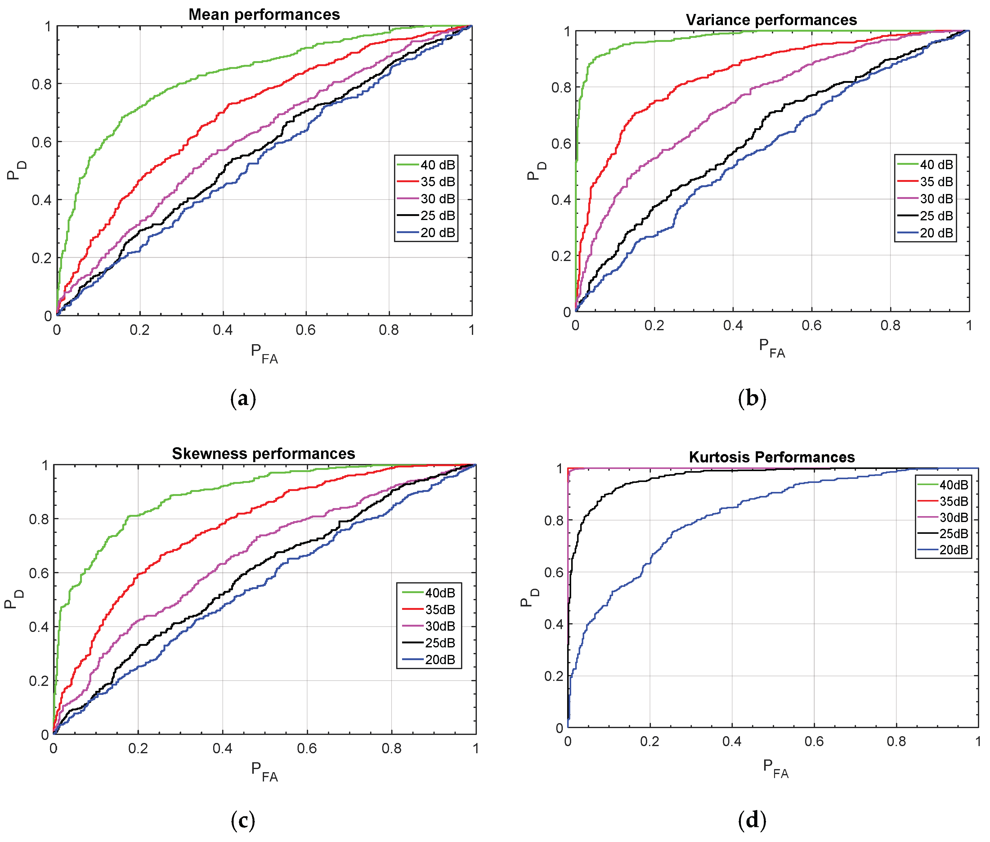
Figure 9 shows the evolution regarding the SNR value for a 60 rad/s rotational speed. It clearly shows that the detection performances are poorer when the noise level increases (SNR decreases). Among the four criteria, the kurtosis offers the best performances even while the noise varies.
With these ROC curves, we can derive an optimal fault detection threshold for these features, which leads to the best trade-off value between PD and PFA. It is clear that, while the noise conditions become more severe (SNR decreases), the optimal fault detection will lead to PD < 0.7 and PFA > 0.3.
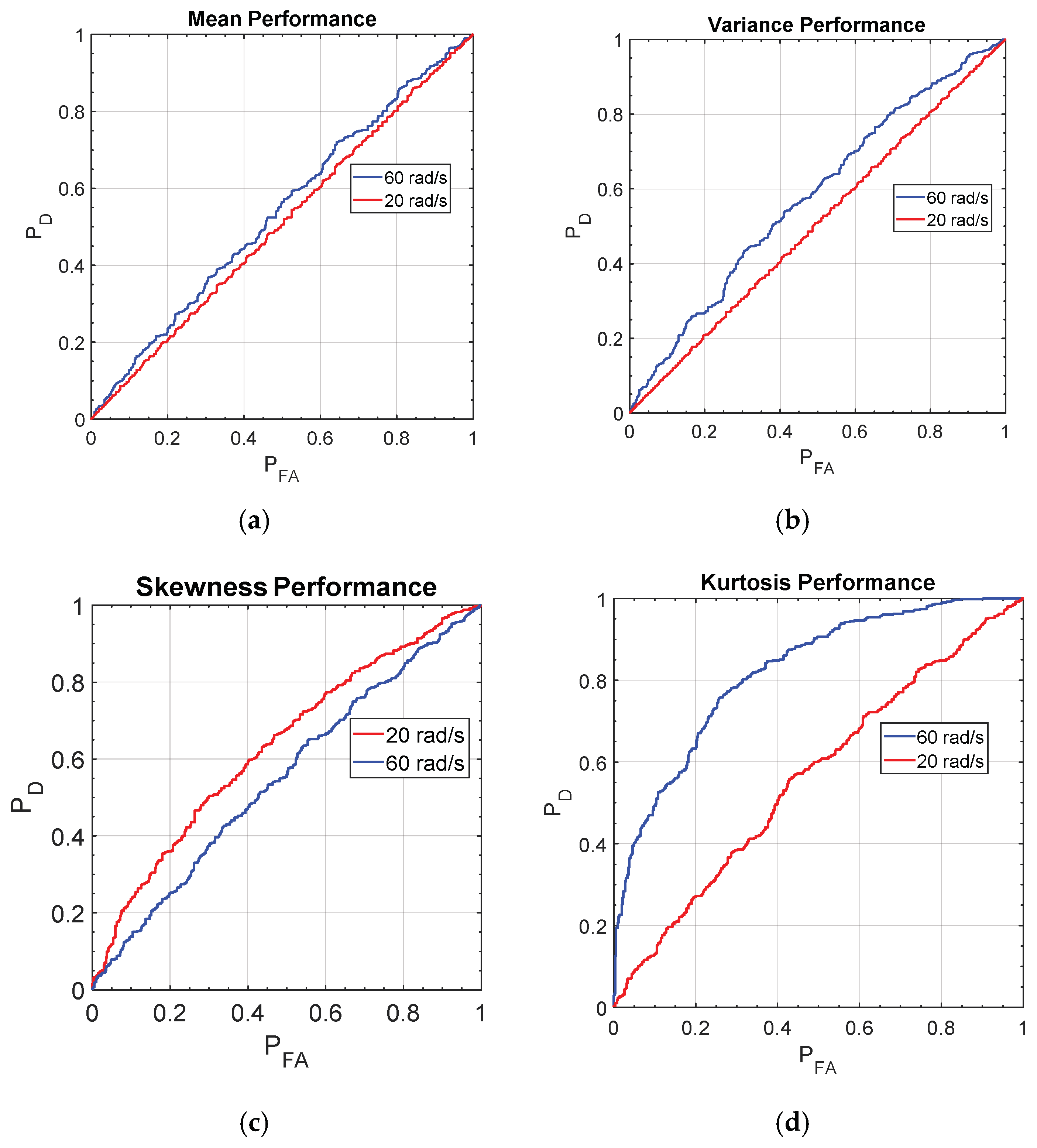
Figure 10 displays the influence of the drive rotational speed on the first four statistical moments for SNR = 20 dB.
Figure 10 shows the degradation of the detection performances when the speed is reduced and the noise is increased. Most of the statistical criteria fail to detect the fault under these conditions. The optimal threshold will generally lead to poor performances PD = 0.56 and PFA = 0.44, which is far from the usual industrial settings (PD > 0.8 and PFA < 0.05). Even the performances for the kurtosis are not satisfying and should be improved in such severe operating conditions.
In most of the faulty cases, the mean value is not a relevant fault indicator. It will not be retained in the following analysis.
To summarize the detection ability for the 10 selected Open Switch fault cases in all the operating conditions (load, noise, and speed), we present in Table 2 the number of faults correctly detected using at least one of the three significant statistical criteria (σ2, Skew, Kurt).
For this analysis, we consider that the fault is correctly detected if PD > 0.8 and its PFA < 0.05.
Table 2 confirms that the detection with the three statistical moments (variance, skewness, and kurtosis) is satisfying for high SNR (SNR ≥ 30 dB) and for high-speed conditions (≥40 rad/s). In these cases, most of the OSFs are detected from the lowest to the highest durations.
Boxes in blue color show cases where performance is considered insufficient with a probability of detection PD < 0.5. In the other conditions (SNR < 30 dB, 20 rad/s), lots of faults are not detected. To enhance the detection performances in such conditions, we propose to improve the features statistical analysis.

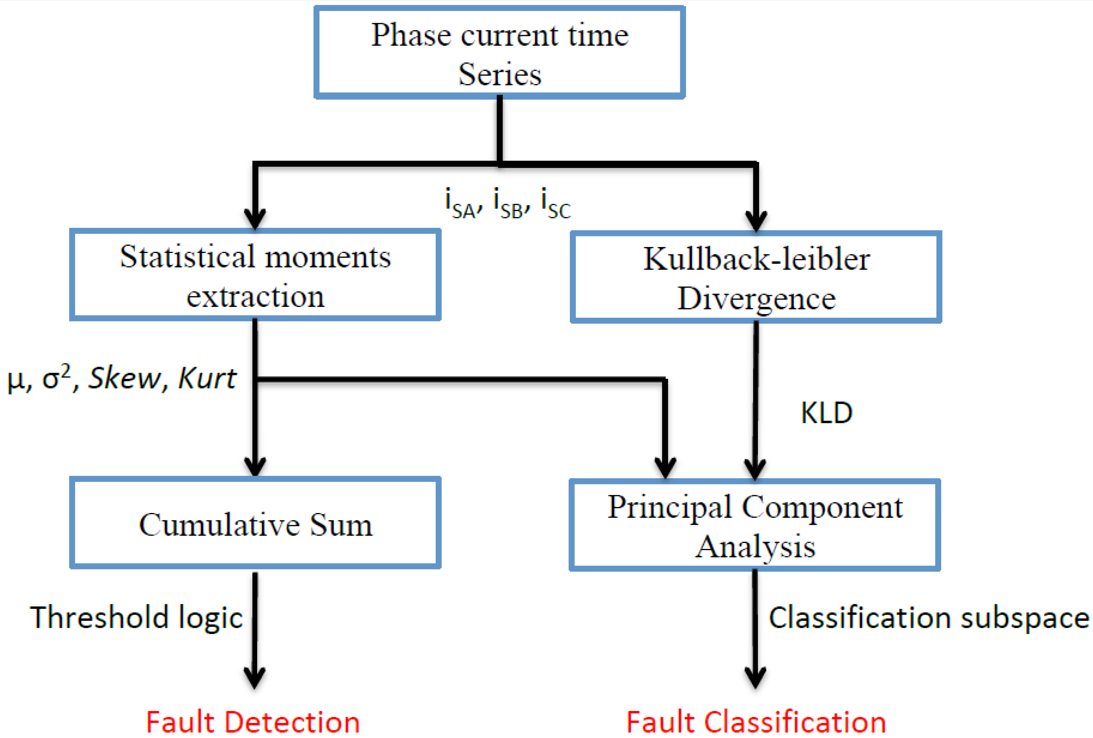
4.2.2. Fault Detection Improvement with CUSUM

To improve the detection in fault detection and the diagnosis process, we propose to combine the statistical features with a Cumulative Sum (CUSUM) analysis.
CUSUM is a well-known technique that has been widely used to detect abrupt changes [21,22,23] in signal processing. It is based on the log-likelihood ratio and has been theoretically defined for mean or variance variation in the considered signal. Optimally, it can be defined for Gaussian signals as the sum of the sufficient statistics sk such as:
S N = k = 1 k = N s k
where N is the number of realizations and sk can be considered in the case of mean changes ( s k μ ) or variance changes ( s k σ ) for the statistical moments signals such as:
s k µ = ( µ f µ h σ 2 ) × ( x k µ f + µ h 2 )
s k σ = ln σ h σ f + ( 1 σ h 2 1 σ f 2 ) × ( x k µ h ) 2 2
where μh and μf are, respectively, the mean values in the healthy and faulty conditions, σh and σf are, respectively, the standard deviation values in healthy and faulty conditions, and xk stands for the statistical moment under consideration for the kth observation over N. While computing the CUSUM SN, we can then set a threshold Th = 0.99Smax where Smax = max(SN) is the maximum value of SN in a healthy case. If the CUSUM value is higher than Th, then it means that a faulty behavior has been detected.
In our work, the considered signals to apply the CUSUM are, hereafter, the ones obtained for 1000 realisations of the previously studied statistical moments (μ, σ2, Skew, Kurt). To consider that the optimal conditions are satisfied, we have first evaluated these realisations-dependent signals using the Kolmogorov-Smirnov test to validate the Gaussian assumption.
Second, the CUSUM is computed for the statistical moment’s signals. As has been concluded in the previous section that the kurtosis is the most sensitive criteria among the four, we focus our next analysis on the CUSUM of this signal. The most severe faulty conditions are particularly studied.
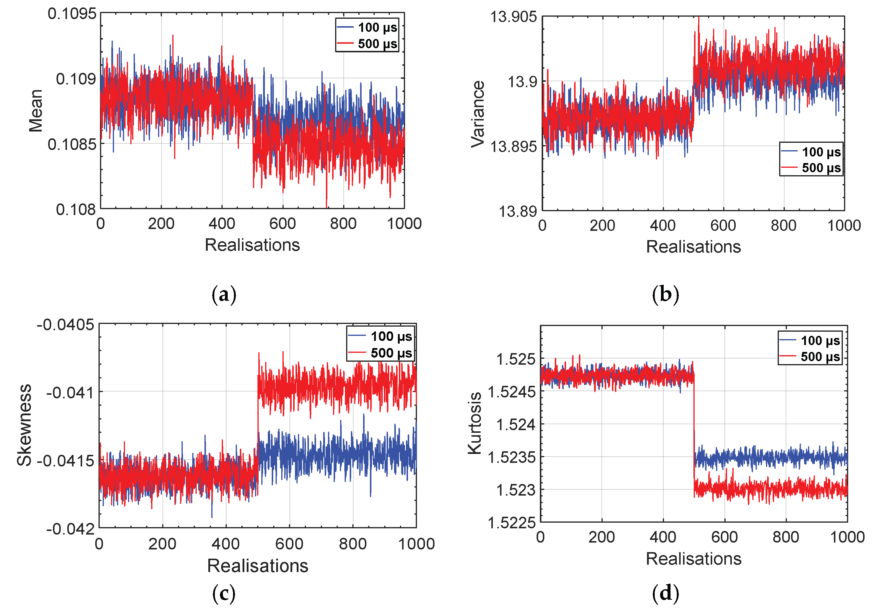
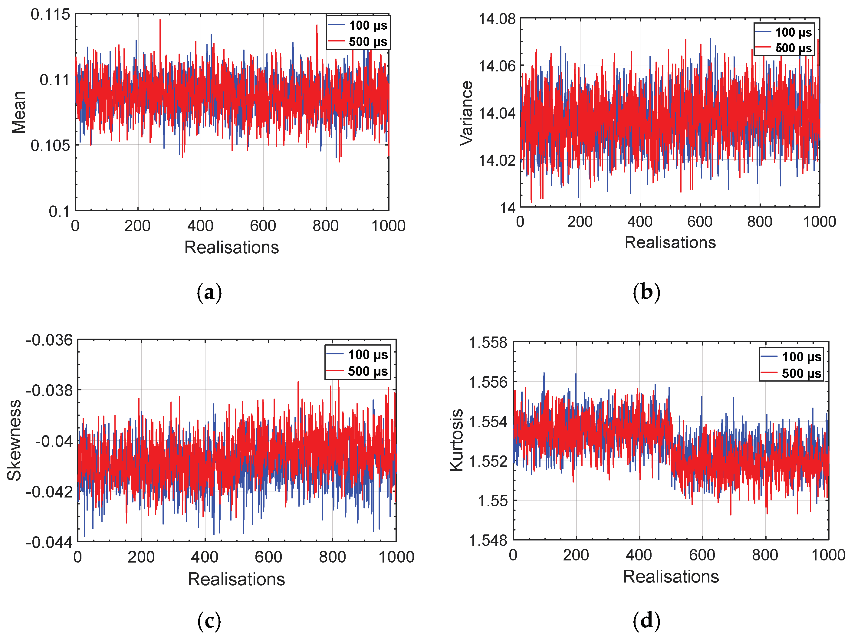
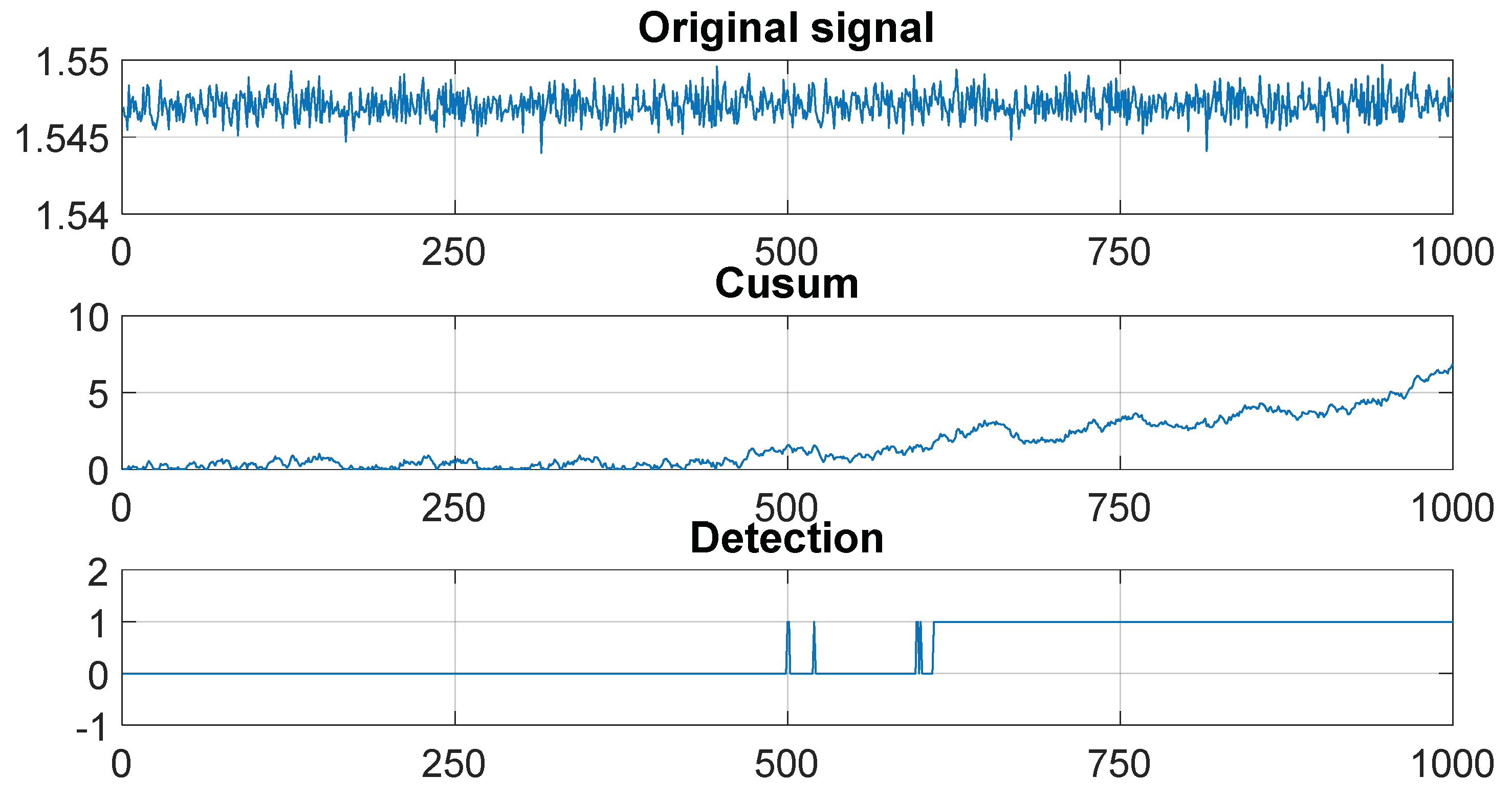
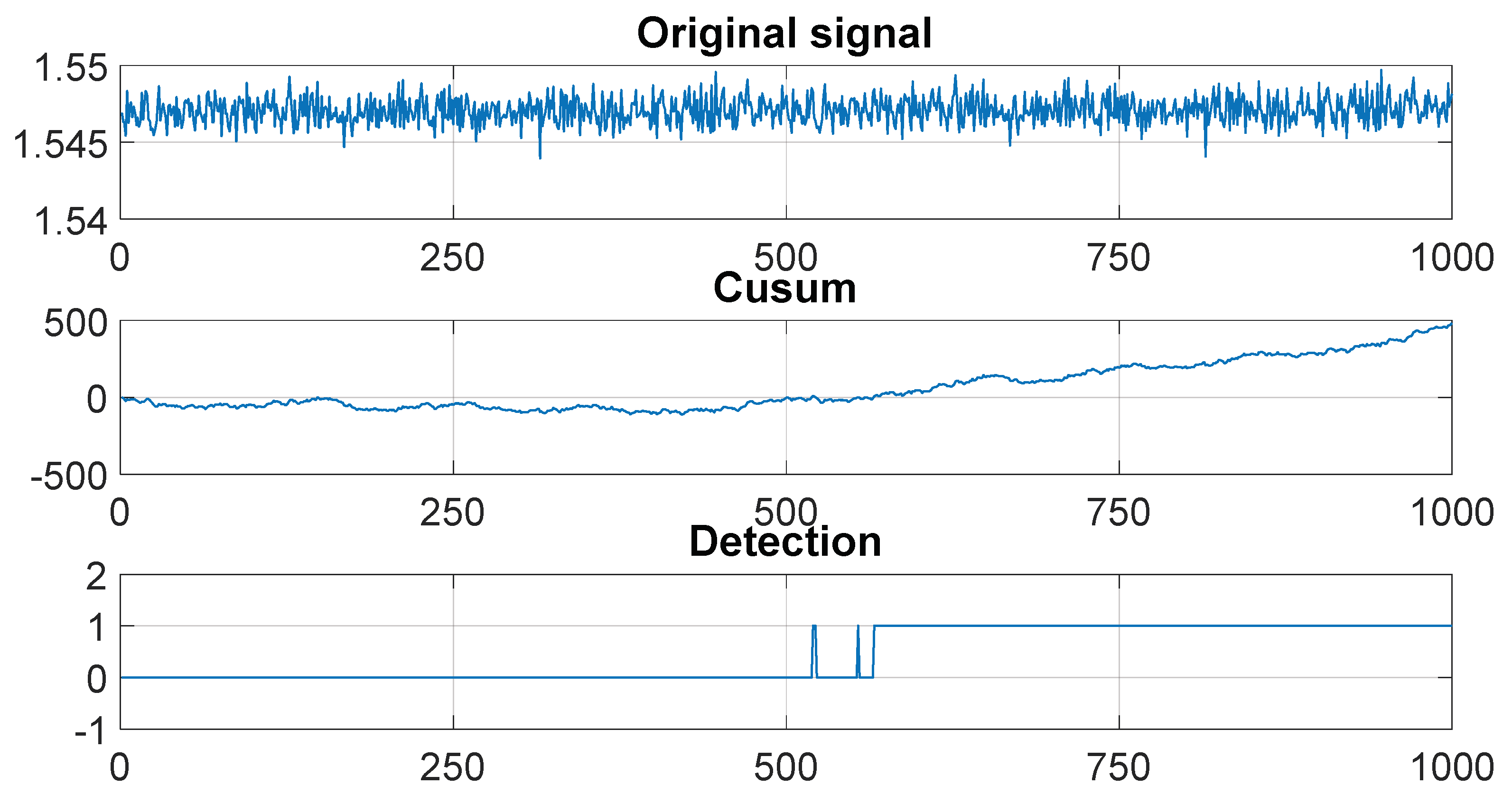
Figure 11 and Figure 12 show, respectively, the CUSUM results for s k µ and s k σ of the kurtosis signal when SNR = 20 dB at 20 rad/s for 100% of the rated load. For the considered signals, the first 500 samples represent the healthy condition and the last 500 represent the faulty ones.
The fault occurrence can be detected efficiently with both indicators. The kurtosis CUSUM signal starts increasing at the fault detection. Nevertheless, one can notice that several (110) faulty realizations (Figure 11) are required for s k μ and 65 faulty ones for s k σ (Figure 12) before fault detection. In the given example, there is no false alarm using s k σ and only one using s k μ .
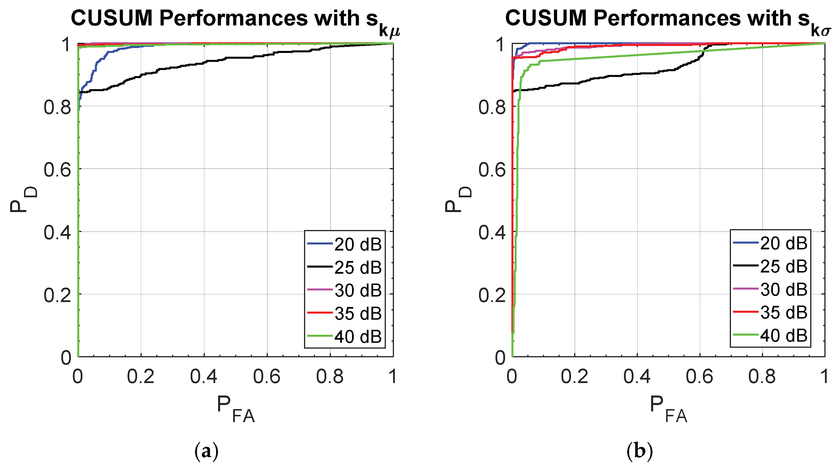
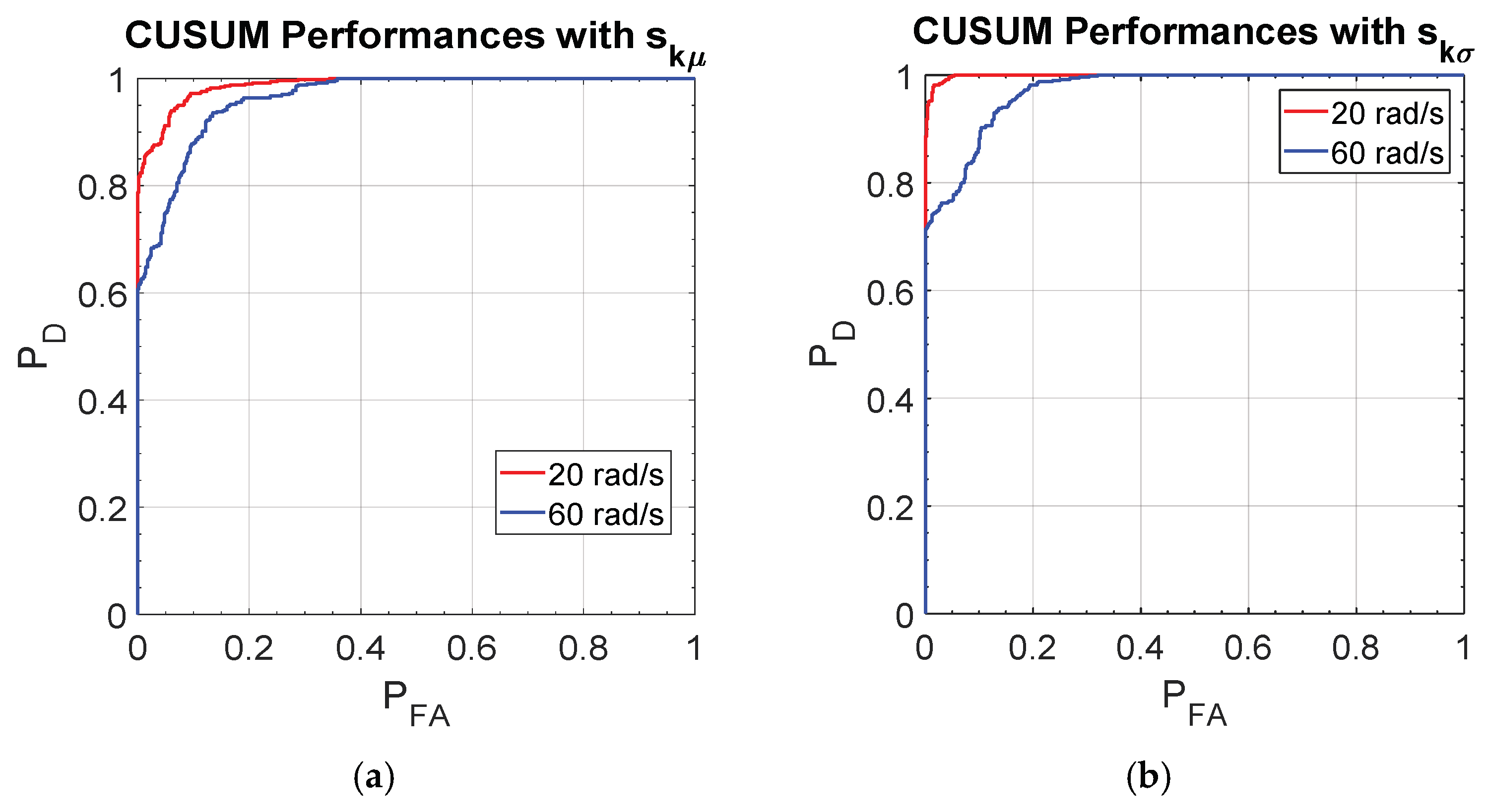
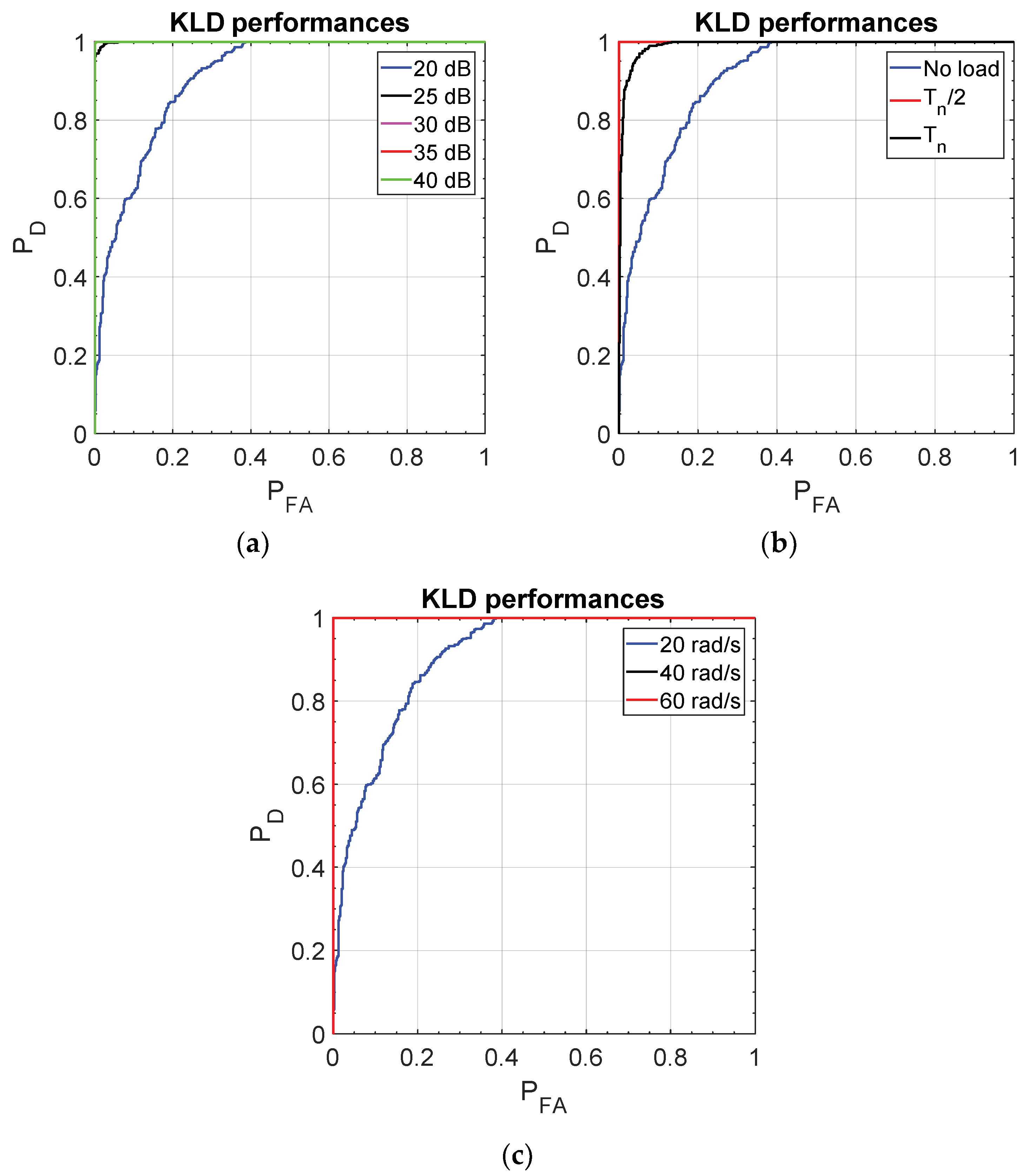
To completely evaluate the detection efficiency using the kurtosis CUSUM, the ROC curves are computed for several operating conditions. As an example, Figure 13 and Figure 14 display the fault detection performance results using s k σ and s k μ for the smallest OSF duration (100 µs), 50% of load, and several noise and speed conditions.
These figures clearly show the improved fault detection performances when compared to those obtained with the straight analysis of the first four statistical moments. Even when the speed and the SNR are low (20 rad/s and 20 dB), the detection is possible and the performances are good with a high detection probability and a low probability of false alarm.
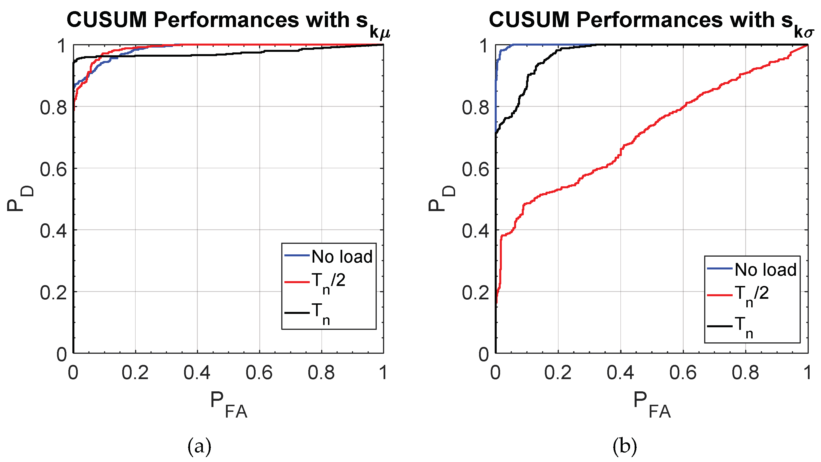
The influence of the load on kurtosis CUSUM for fault detection is plotted in Figure 15. The results show that s k σ is more sensitive to load variations particularly at half load where the performances are poor. At no load and full load, the performances are good.
As a summary, the fault detection results with the kurtosis CUSUM (with s k μ or s k σ ) are presented in Table 3 and Table 4 considering the 10 OSF for different operating conditions.
Boxes in blue color show cases where performance is considered as insufficient with a probability of detection PD < 0.5.
Using the cumulative sum, the detection performances are largely improved. All the OSF, even the most incipient one (with 100 µs duration) can at least be detected using one of the CUSUM information based on the kurtosis signal. The detection can be performed but the fault classification, according to the fault duration cannot be obtained.
In the following, we propose a solution to classify the detected faults, according to their durations.

5. Fault Classification

The following classification procedure is supported by the methodology described by the flowchart depicted in Figure 6.

5.1. Features Extraction for Fault Classification

From the previous sections, we have deduced that the first four statistical moments extracted from the current flowing in the machine windings are not sufficient especially in the case of the incipient faults. Therefore, we propose to combine them with a distance measure [24], the Kullback-Leibler divergence (KLD).
The Kullback–Leibler Divergence (KLD), or the relative entropy, is a well-known probabilistic tool that has proven its worth in machine learning, neuroscience, pattern recognition [25], and anomaly detection [26,27]. KLD has already proved its efficiency for detecting incipient faults in several applications [28,29].
Its main goal is the evaluation of the divergence of two signals based on their probability distribution functions (pdf).
Theoretically, for two pdfs f(x) and g(x) of continuous random variable x, Kullback and Leibler have defined the Kullback-Leibler Information from f to g [17] as:
I ( f g ) = f ( x ) log f ( x ) g ( x ) d x
The KLD is defined as the symmetric version of the Information [15,21] denoted as:
K L D ( f , g ) = I ( f g ) + I ( g f )
Following Reference (5), the KLD is assumed non-negative and null if and only if the two distributions are strictly the same. One of the main constraints of this technique is that the two distributions have to share the same support set.
Hereafter, we propose to use the KLD to identify the divergence between healthy and faulty cases of the phase current time series (see Figure 16). At first, the KLD is computed 500 times between the distributions of different realisations of healthy signals obtained in the same operating conditions with a reference one. Then at second, the KLD is computed 500 times between the reference healthy signal and different realisations of the faulty signals.
As an example, the KLD results for three different durations of the Open-Switch Fault for one of the critical cases previously studied (20 rad/s, 50% of Tn, SNR = 20 dB) are depicted in Figure 17. The first 500 realizations represent the KLD in healthy conditions (no faults) and the last 500 realizations represent the KLD in faulty conditions.
As can be noticed when looking at Figure 17, for the three faults (100 µs, 200 µs, and 500 µs), a significant variation of the KLD is observed. All the faults can be detected with a detection probability PD ≥ 0.98 when using an optimal threshold.
To evaluate the efficiency of the KLD more accurately, the ROC curves have been computed in different operating conditions for the most incipient fault (100 µs). The performances are plotted in Figure 18.
Based on the results in Figure 18, we can draw the following conclusions:
  • At 60 rad/s, the fault detection with KLD is almost perfect (PD = 1) with no false alarms regardless of the noise level, the fault duration, and the load.
  • At 40 rad/s, the performances are slightly degraded for 100 µs fault duration (PD > 0.98 for 50% and 100% of load and PD = 0.82 for no load) but remain excellent.
  • At 20 rad/s, the performances are slightly reduced, but they are still acceptable.
Table 5 summarizes the performances obtained for the KLD. Boxes in blue color show cases where performance is considered insufficient with a probability of detection PD lower than 0.5.
The results previously obtained have shown the ability to detect OSF with different durations thanks to the combination of several statistical criteria (statistical moments and KLD). However, we cannot retrieve fault classification information from these results.

5.2. Feature Analysis for Fault Classification

In this section, we propose (see Figure 6) to combine these criteria in a multivariate analysis using PCA for fault classification and identification.
PCA is a multivariate tool that can be used in a descriptive way to highlight the similarities in a dataset and then allow the classification purpose. This tool has been widely used for fault diagnosis and has proven its efficiency if the information in the dataset can be linearly separated [30,31]. For this technique, the data is arranged in a database where several features are arranged as variables describing a huge number of observations (samples) in the different operating conditions.
Principal component analysis (PCA) is a statistical procedure that uses an orthogonal transformation to convert the set of observations of possibly correlated variables into a set of linearly, uncorrelated variables called principal components (PC).
In the following:
  • m is the number of features or variables. In our case m = 5 with (μ, σ 2, Skew, Kurt, KLD);
  • N is the number of samples for each variable for all operating conditions, including healthy and faulty cases.
The m variables (features) are organized in a matrix X[N×m]. X is then composed of m column vectors X = (x1, …xj, …xm). The line vector (xi)j (j = 1, ….m) ∈ m is the ith measurement of the m variables.
The main goal of the PCA consists of looking for an orthogonal transformation of the auto scaled matrix of X noted X ¯ into a new matrix TN×m of uncorrelated variables t1, t2,…, tm named principal component scores, T = [t(1),, t(i),, t(N)]’ where t(i) ∈ m , in order to obtain new variables that are linear combinations of the original ones with a maximum total data variance. The vectors of T matrix are obtained using the eigenvectors of the correlation matrix. These eigenvectors are arranged as columns of a matrix P[m×m] in the descendent order of their corresponding eigenvalues, then T is obtained as T = PX.
In this work, we have considered the five variables (μ, σ 2, Skew, Kurt, KLD) and 500 realizations of each variable in each studied condition. Then, we obtain five principal components in each group. With this method, we will evaluate how the samples can be grouped, and if the faults can be classified properly for the same operating conditions.
The first study is done with the collected data from the 10 OSF and SNR = 20dB considering low speed conditions (20 rad/s) and the three load conditions (0%, 50%, and 100% of the rated torque). The PCA framework is obtained and the first two vectors of the matrix T are denoted as the principal components (PC1 and PC2). They cumulate more than 75% of the total variance and will be, therefore, used to represent the data samples. Therefore, in the following section, we will retain the first two principal components that represent most of the information of the original dataset. The PCA results are displayed in Figure 19.
From Figure 19, we can see that the higher the load is (from 0% to 100% of the rated torque), the better the classification (less overlapping) of the OSF according to their durations (from 0 to 1 ms with a 100 µs step) will be. The obtained groups intra-class variances clearly decrease from Figure 19a to Figure 19c. The efficiency of the fault duration classification is widely influenced by the drive load variation. In full load conditions, the system faulty behaviour can be perfectly distinguished from the healthy one in the 2-dimension PC feature space.
To highlight the effect of the speed evolution on the fault classification, we propose in Figure 20 the PCA results for a speed of 60 rad/s at the rated load. The first two first principal components represent 97.47% of the total information. The separation of the 11 groups (healthy and 10 faulty ones) based on their duration is almost perfect.
The same trend is obtained for a speed of 40 rad/s. Therefore, the more the speed is, the higher and better will be the fault classification results.
The application of PCA as a feature analysis tool for the fault classification is efficient. The method allows the classification of incipient Open-Switch faults (corresponding to at least one switching period at 10 kHz) with only the first and the second principal component at 40 and 60 rad/s. For 20 rad/s motor speed, the performances can be improved with the use of more than two principal components.

6. Conclusions

This paper deals with intermittent Open-Switch fault detection and classification for a three-level NPC inverter-fed Induction Motor Drive. For this work, the time series phase currents are used as input data for the Fault Detection and Diagnosis. Different operating conditions (noise, speed, and load) for several fault durations are considered. The proposal is based on the statistical features extracted from the input data.
At first, we have used the first four statistical moments as fault features. Based on these features, the fault is properly detected with a probability of detection higher than 0.8 when the rotating speed is higher than one-third of the nominal speed. The results have also shown that the kurtosis is the most efficient criteria for all the operating conditions. As for the other evaluated statistical moments, its performance is degraded at lower speed and for lower SNR (high noise levels). The results have shown that the operating conditions widely influence the fault detection. Based on the performance evaluation for these features, it has been shown that, for high noise levels at low speed and in variable load conditions, the fault detection becomes more difficult. Moreover, the lower the fault duration is, the lower the fault detection efficiency becomes.
To improve the detection performances, we have proposed in a second step to combine the kurtosis with the Cumulative Sum algorithm. The detection performance for the incipient faults has been significantly improved in the most severe conditions (low speed and high noise).
The third step of this work was the evaluation of the Kullback-Leibler divergence (KLD) for fault detection. Based on the comparison of one period of the current signal probability density function in healthy and faulty conditions, the method is efficient and offers the best detection performances whatever the operating conditions. Unfortunately, these performances do not allow us to perfectly identify the faults whatever the environment.
Finally, the last step was the fault classification. The proposed method is based on Principal Component Analysis using the previously studied features (statistical moments and Kullback-Leibler divergence). The classification is then performed using the first two principal components that contain most of the information of the original database. The faults are properly classified, according to their duration and for the considered operating conditions (speed, load, and noise level).

Author Contributions

Methodology, C.D. and D.D. Software, M.B. Supervision, C.D. and D.D. Writing—original draft, M.B., C.D., and D.D. Writing—review & editing, C.D., D.D., A.H., D.M., and T.W.

Funding

This research received no external funding.

Conflicts of Interest

The authors declare no conflict of interest.

Nomenclature

Acronyms
NPCNeutral-Point Clamped
IMInduction Machine
SCFShort Circuit Fault
OSFOpen Circuit Fault
FDDFault Detection and Diagnosis
EUDCEuropean Driving Cycle
CUSUMCumulative SUM
PCAPrincipal Component Analysis
SNRSignal to Noise Ratio
KLDKullack-Leibler Divergence
Variables
μmean value
σ2variance
SkewSkewness
KurtKurtosis
PDprobability of fault detection
PFAprobability of false alarm
XNxmdata matrix
va, vb, vcphase voltages
iSA, iSB, iSCphase currents
IKullback-Leibler Information

References

  1. Ganev, E. Selecting the Best Electric Machines for Electrical Power-Generation Systems: High-performance solutions for aerospace more electric architectures. IEEE Electron. Mag. 2014, 2, 13–22. [Google Scholar] [CrossRef]
  2. Chudzikiewicz, A.; Bogacz, R.; Kostrzewski, M.; Konowrocki, R. Condition monitoring of railway track systems by using acceleration signals on wheelset axle-boxes. Transport 2018, 33, 555–566. [Google Scholar] [CrossRef]
  3. Ferguson, M.; Law, K.H.; Bhinge, R.; Lee, Y.T. A generalized method for featurization of manufacturing signals, with application to tool condition monitoring. In Proceedings of the 37th Computers and Information in Engineering Conference IDETC2017, Cleveland, OH, USA, 6–9 August 2017. [Google Scholar]
  4. Chybowski, L.; Gawdzińska, K. On the Possibilities of Applying the AHP Method to a Multi-criteria Component Importance Analysis of Complex Technical Objects. Adv. Intell. Syst. Comput. 2016, 445, 701–710. [Google Scholar]
  5. Benbouzid, M.; Delpha, C.; Khatir, Z.; Lefebvre, S.; Diallo, D. Faults Detection and Diagnosis in a Static Converter. In Electrical Machines Diagnosis; Wiley: New York, NY, USA, 2011; pp. 271–316. [Google Scholar]
  6. Franquelo, L.; Rodriguez, J.; Leon, J.I.; Kouro, S.; Portillo, L.; Prats, M. The age of Multilevel Converter arrives. IEEE Ind. Electron. Mag. 2008, 2, 28–39. [Google Scholar] [CrossRef]
  7. Abu-Rub, H.; Malinowski, M.; Al Haddad, K. Multilevel Converter/Inverter Topologies and Applications; Wiley-IEEE Press: New York, NY, USA, 2014. [Google Scholar]
  8. Sharkh, S.M.; Abusara, M.A.; Orfanoudakis, G.I.; Hussain, B. Power Electronic Converters for Microgrids; IEEE Wiley: New York, NY, USA, 2014; 72p. [Google Scholar]
  9. Wu, B.; Narimani, M. Diode-Clamped Multilevel Inverters; Wiley-IEEE Press: New York, NY, USA, 2017. [Google Scholar]
  10. Chowdhury, A. Three-Level Neutral Point Clamped Traction Inverter Drive for Electric Vehicles. Ph.D. Thesis, Concordia University, Montreal, QC, Canada, April 2015. [Google Scholar]
  11. Errabelli, R.; Mutschler, P. Fault-tolerant voltage source inverter for permanent magnet drives. IEEE Trans. Power Electron. 2012, 27, 500–508. [Google Scholar] [CrossRef]
  12. Varghese, S.E.; Reema, N. Effects of Switching Faults on Induction Motor Drive System. IRJET 2016, 3, 607–611. [Google Scholar]
  13. Delpha, C.; Diallo, D.; Al Samrout, H.; Moubayed, N. Multiple incipient fault diagnosis in three-phase electrical systems using multivariate statistical signal processing. Eng. Appl. Artif. Intell. 2018, 73, 68–79. [Google Scholar] [CrossRef]
  14. Lezana, P.; Pou, J.; Meynard, T.A.; Rodriguez, J.; Ceballos, S.; Richardeau, F. Survey on Fault Operation in Multilevel Inverters. IEEE Trans. Ind. Electron. 2010, 57, 2207–2218. [Google Scholar] [CrossRef]
  15. Lamb, J.; Mirafzal, B. Open-Circuit IGBT Fault Detection and Location Isolation for Cascaded Multilevel Inverters. IEEE Trans. Ind. Electron. 2017, 64, 4846–4853. [Google Scholar] [CrossRef]
  16. Rothenhagen, K.; Fuchs, F.W. Performance of diagnosis methods for IGBT open circuit faults in voltage source active rectifiers. In Proceedings of the IEEE PESC, Aachen, Germany, 20–25 June 2004; pp. 4348–4354. [Google Scholar]
  17. Mendes, A.M.S.; Cardoso, A.J.M.; Saraiva, E.S. Voltage source inverter fault diagnosis in variable speed AC drives, by the average current Park’s vector approach. In Proceedings of the IEEE IEMDC, Seattle, WA, USA, 9–12 May 1999; pp. 704–706. [Google Scholar]
  18. Kullback, S.; Leibler, R.A. On information and sufficiency. Ann. Math. Stat. 1951, 22, 79–86. [Google Scholar] [CrossRef]
  19. Jolliffe, I. Principal Component Analysis, 2nd ed.; Springer Series in Statistics: London, UK, 2002. [Google Scholar]
  20. Green, D.M.; Swets, J.M. Signal Detection Theory and Psychophysics; John Wiley and Sons Inc.: New York, NY, USA, 1966. [Google Scholar]
  21. Blanke, M.; Kinnaert, M.; Lunze, J.; Staroswiecki, M. Diagnosis and Fault-Tolerant Control, 2nd ed.; Springer: Berlin, Germany, 2006; pp. 238–263. [Google Scholar]
  22. Basseville, M.; Nikiforov, I. Detection of Abrupt Changes-Theory and Applications; Prentice-Hall: Englewood Cliffs, NJ, USA, 1993. [Google Scholar]
  23. Delpha, C.; Diallo, D.; Al Samrout, H.; Moubayed, N. Incipient fault detection and diagnosis in a three-phase electrical system using statistical signal processing. In Proceedings of the IEEE Industrial Electronics Conference (IECON 2017), Beijing, China, 29 October–1 November 2017; pp. 3828–3833. [Google Scholar]
  24. Basseville, M. Distances measures for signal processing and pattern recognition. Signal Process. 1989, 18, 349–369. [Google Scholar] [CrossRef]
  25. Silva, J.; Narayanan, S. Average divergence distance as a statistical discrimination measure for hidden Markov models. IEEE Trans. Audio Speech Lang. Process. 2006, 14, 890–906. [Google Scholar] [CrossRef]
  26. Afgani, M.; Sinanovic, S.; Haas, H. Anomaly detection using the Kullback–Leibler divergence metric. In Proceedings of the 1st International Symposium on Applied Science on Biomedical and Computer Technology (ISABEL 2008), Aalborg, Denmark, 25–28 October 2008. [Google Scholar]
  27. Anderson, A.; Hass, H. Kullback–Leibler divergence (KLD) based anomaly detection and monotonic sequence analysis. In Proceedings of the IEEE Vehicular Technology Conference (VTCFall), Budapest, Hungary, 15–18 May 2011. [Google Scholar]
  28. Harmouche, J.; Delpha, C.; Diallo, D. Incipient Fault Detection and Diagnosis Based on Kullback-Leibler Divergence Using Principal Component Analysis: Part I. Signal Process. 2014, 94, 278–287. [Google Scholar] [CrossRef]
  29. Chai, Y.; Tao, S.; Mao, W.; Zhang, K.; Zhu, Z. Online incipient fault diagnosis based on Kullback-Leibler divergence and recursive principle component analysis. Can. J. Chem. Eng. 2018, 96, 426–433. [Google Scholar] [CrossRef]
  30. Zuo, M.J.; Lin, J.; Fan, X. Feature separation using ICA for a one-dimensional time series and its application in fault detection. J. Sound Vib. 2005, 287, 614–624. [Google Scholar] [CrossRef]
  31. Harmouche, J.; Delpha, C.; Diallo, D. Incipient Fault Detection and Diagnosis Based on Kullback-Leibler Divergence Using Principal Component Analysis: Part II. Signal Process. 2015, 109, 334–344. [Google Scholar] [CrossRef]
Figure 1. Block diagram of the induction machine drive.
Energies 12 01372 g001
Figure 2. Three-level NPC inverter.
Energies 12 01372 g002
Figure 3. Phase current with a permanent OSF.
Energies 12 01372 g003
Figure 4. Intermittent 500 µs Open-Switch fault impact: (a) Phase current waveforms in healthy and faulty cases. (b) Electromagnetic torque in healthy and faulty cases.
Energies 12 01372 g004
Figure 5. Flowchart for the methodology and its application in our work.
Energies 12 01372 g005
Figure 6. Flowchart of the fault detection and fault classification.
Energies 12 01372 g006
Figure 7. Statistical moments for two OSF durations with SNR = 40 dB: (a) With mean value, (b) With variance, (c) With Skewness, (d) With Kurtosis.
Energies 12 01372 g007
Figure 8. Statistical moments for two OSF durations with SNR = 20 dB: (a) With mean value, (b) With variance, (c) With Skewness, (d) With Kurtosis.
Energies 12 01372 g008
Figure 9. Open switch fault (duration 100 µs) detection performance for 60 rad/s at rated torque: (a) With mean value, (b) With variance, (c) With Skewness, (d) With Kurtosis.
Energies 12 01372 g009
Figure 10. Open switch fault (duration 100 µs) detection performance with SNR = 20 dB: (a) With mean value, (b) With variance, (c) With Skewness, (d) With Kurtosis.
Energies 12 01372 g010
Figure 11. Fault detection results with the mean value.
Energies 12 01372 g011
Figure 12. Fault detection results with the variance value.
Energies 12 01372 g012
Figure 13. 100 µs OSF detection performance for 20 rad/s and 50% of the load: (a) With mean value, (b) With variance.
Energies 12 01372 g013
Figure 14. 100 µs OSF detection performance for SNR = 20dB and 50% of the load: (a) With mean value, (b) With variance.
Energies 12 01372 g014
Figure 15. 100 µs OSF detection performance for SNR = 20 dB at 20 rad/s: (a) With the mean value, (b) With the variance.
Energies 12 01372 g015
Figure 16. Flowchart for application of the KLD.
Energies 12 01372 g016
Figure 17. KLD results for 3 OSF at 20 rad/s, 50% of load and SNR = 20 dB.
Energies 12 01372 g017
Figure 18. KLD performances for OSF 100 µs with: (a) 20 rad/s, 0% of load, (b) SNR = 20 dB, 20 rad/s, and (c) SNR = 20 dB.
Energies 12 01372 g018
Figure 19. PCA results for 20 rad/s motor speed and SNR = 20 dB: (a) no load, (b) half rated load, and (c) full load.
Energies 12 01372 g019aEnergies 12 01372 g019b
Figure 20. PCA results for 60 rad/s motor speed at a rated load.
Energies 12 01372 g020
Table 1. Induction machine main characteristics.
CharacteristicsSymbolValueUnit
Nominal voltageUn220/380V
Nominal speedNn1420rpm
Nominal powerPn1.5kW
Rated torqueTn10Nm
Nominal frequencyf50Hz
Number of polesp2
Stator resistanceRs4.85Ω
Rotor resistanceRr3.805Ω
Stator self-inductanceLs0.274H
Rotor self-inductanceLr0.274H
Mutual inductance (stator-rotor)Lm0.258H
InertiaJ0.031kgm2
Table 2. Statistical moments of detection performances with PD > 0.8.
SNR20 rad/s40 rad/s60 rad/s
No Load50% of Tn100% of TnNo Load50% of Tn100% of TnNo Load50% of Tn100% of Tn
40 dB9/104/1010/109/107/1010/1010/1010/1010/10
35 dB7/100/1010/109/109/1010/1010/1010/1010/10
30 dB1/100/1010/108/104/108/1010/1010/109/10
25 dB0/100/106/106/102/106/1010/109/106/10
20 dB0/100/103/102/100/102/109/108/106/10
Table 3. CUSUM mean detection performances for kurtosis signal with PD > 0.8.
SNR20 rad/s40 rad/s60 rad/s
No load50% of Tn100% of TnNo load50% of Tn100% of TnNo load50% of Tn100% of Tn
40 dB6/106/108/105/106/102/107/104/105/10
35 dB5/107/108/106/109/104/108/106/105/10
30 dB6/106/103/106/107/103/108/105/106/10
25 dB5/108/102/105/108/103/109/105/105/10
20 dB9/107/109/107/103/105/109/1010/104/10
Table 4. CUSUM variance detection performances for kurtosis signal with PD > 0.8.
SNR20 rad/s40 rad/s60 rad/s
No load50% of Tn100% of TnNo load50% of Tn100% of TnNo load50% of Tn100% of Tn
40 dB10/109/1010/1010/1010/1010/1010/1010/1010/10
35 dB9/1010/108/1010/1010/1010/1010/1010/1010/10
30 dB10/109/109/1010/109/1010/1010/1010/1010/10
25 dB9/1010/109/109/109/1010/1010/1010/1010/10
20 dB7/108/106/108/108/1010/109/1010/108/10
Table 5. KLD performances with PD > 0.8.
SNR20 rad/s40 rad/s60 rad/s
No load50% of Tn100% of TnNo load50% of Tn100% of TnNo load50% of Tn100% of Tn
40 dB7/107/1010/1010/106/1010/1010/1010/1010/10
35 dB8/103/108/1010/1010/1010/1010/1010/1010/10
30 dB8/108/109/1010/109/109/1010/1010/1010/10
25 dB8/108/108/109/1010/1010/1010/1010/1010/10
20 dB8/105/107/1010/106/1010/109/1010/109/10

