Analyzing the Impact of GDP on CO2 Emissions and Forecasting Africa’s Total CO2 Emissions with Non-Assumption Driven Bidirectional Long Short-Term Memory


Abstract
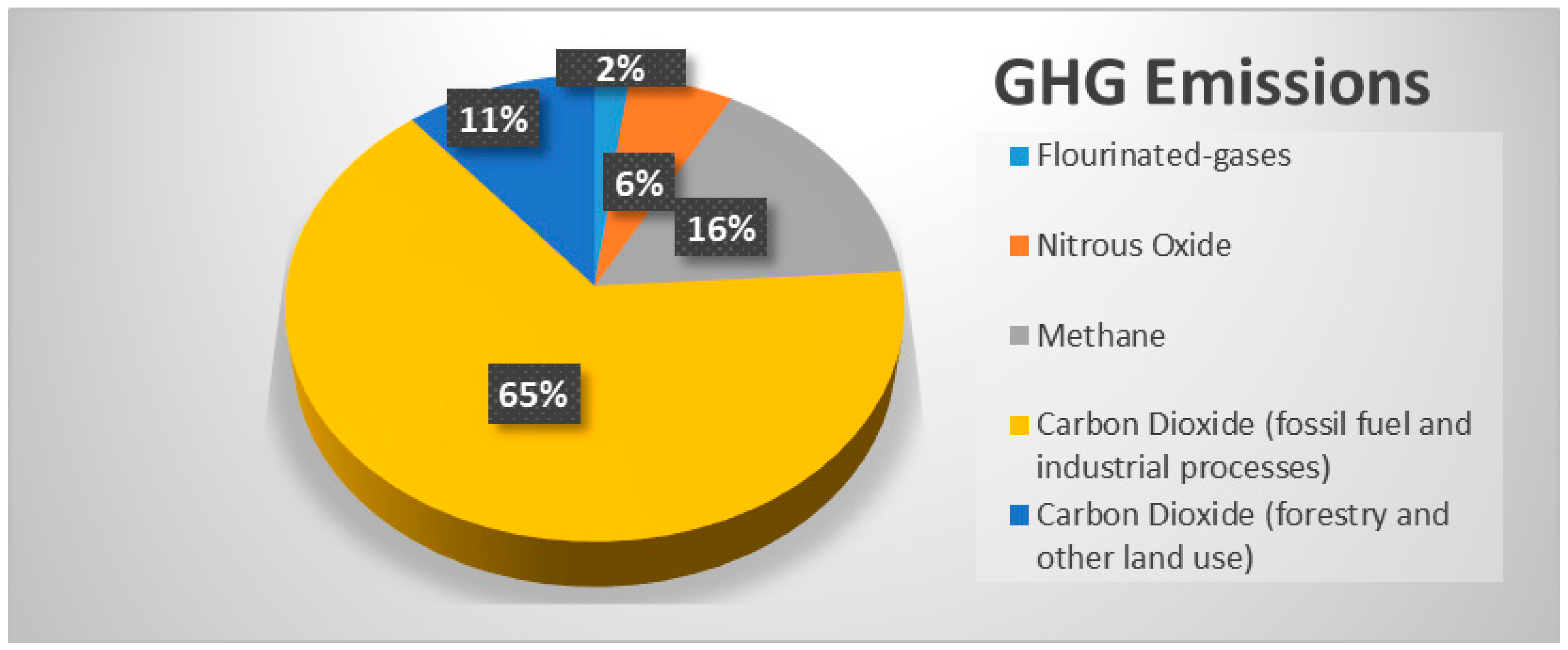
:1. Introduction
2. Materials and Methods
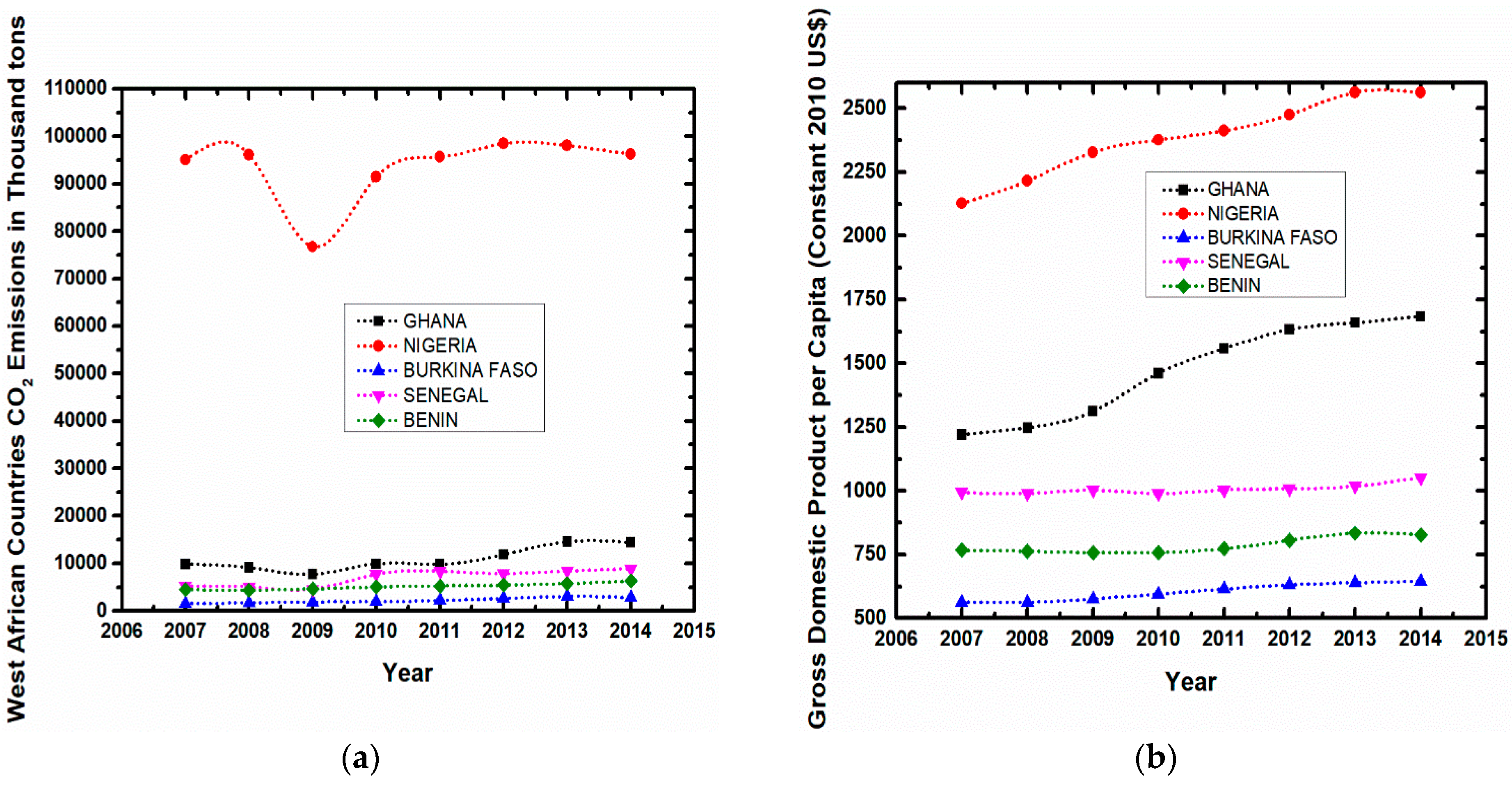
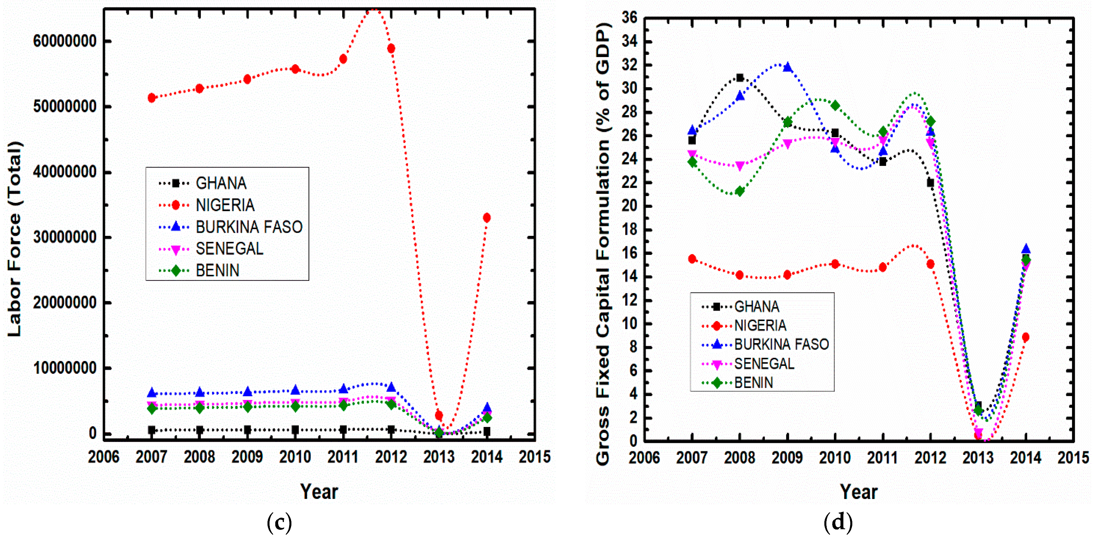
2.1. Data Source for Panel Analysis
2.2. Panel Economic Model Method
2.3. Data Source and Conversion for Training, Testing and Forecasting Stage
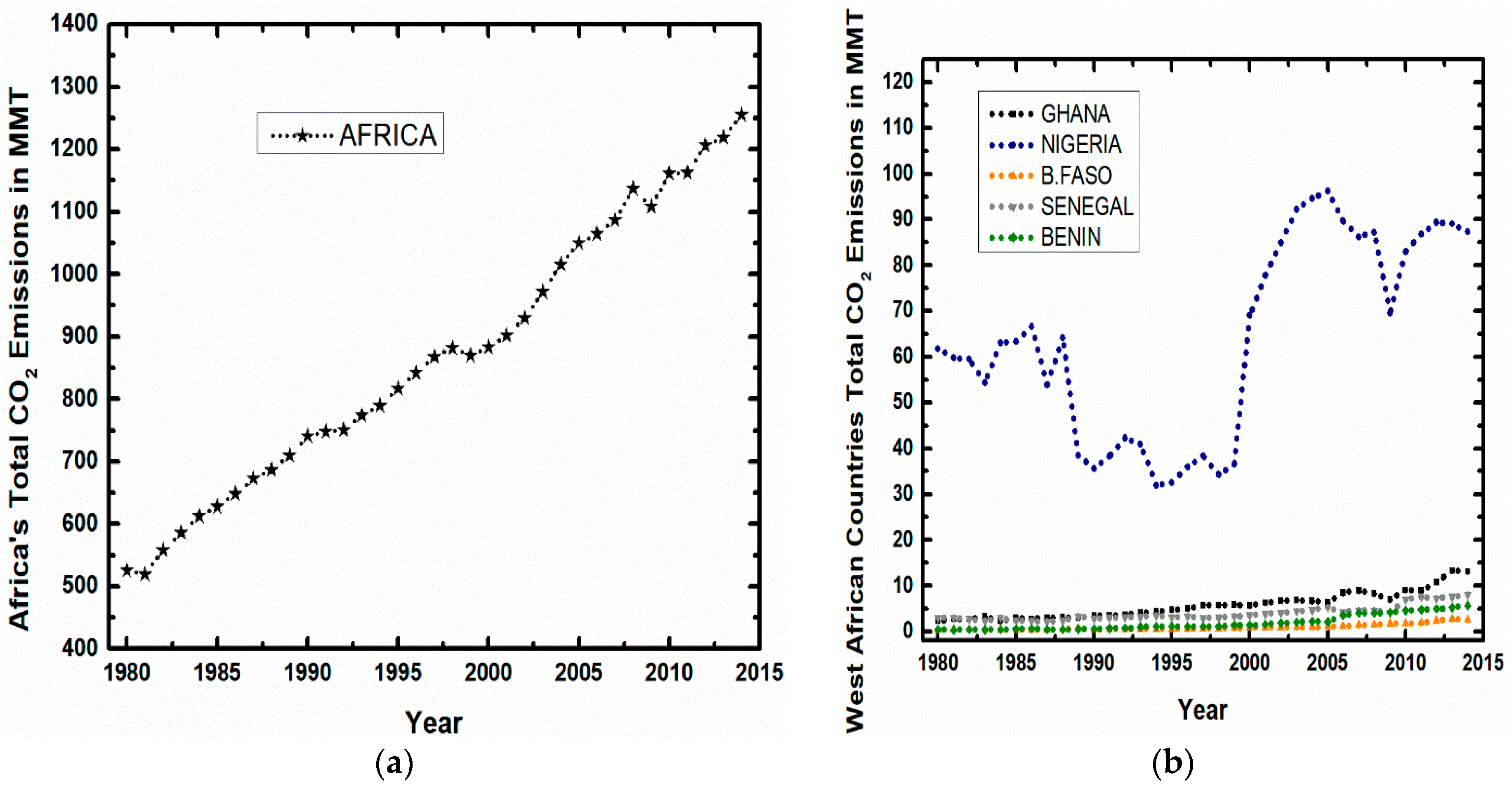
2.4. Bidirectional Long Short-Term Memory (BiLSTM) Algorithm Formulation Processes
- The output from the input layer () is formulated as:where is the hidden weight in the input gate layer and is the input gate biased vector.
- The output from the tanh layer () is formulated as:where is the hidden weight from the tanh layer output and is the tanh layer output biased vector.
- The output from the current cell state of the cell () is formulated as:where is the cell state of the previous cell.
- Our output gate layer () is formulated as:where is the hidden weight in the output gate layer and is the output gate layer biased vector.
- Finally, our hidden vectors () is formulated as:
2.5. Error Indexes
3. Empirical Panel Data Analysis
3.1. Cross-Sectional Dependence Analysis
3.2. Stationarity Analysis
3.3. Panel Co-Integration Test
3.4. Granger Causality Analysis
4. BiLSTM Testing and Forecasting Analysis
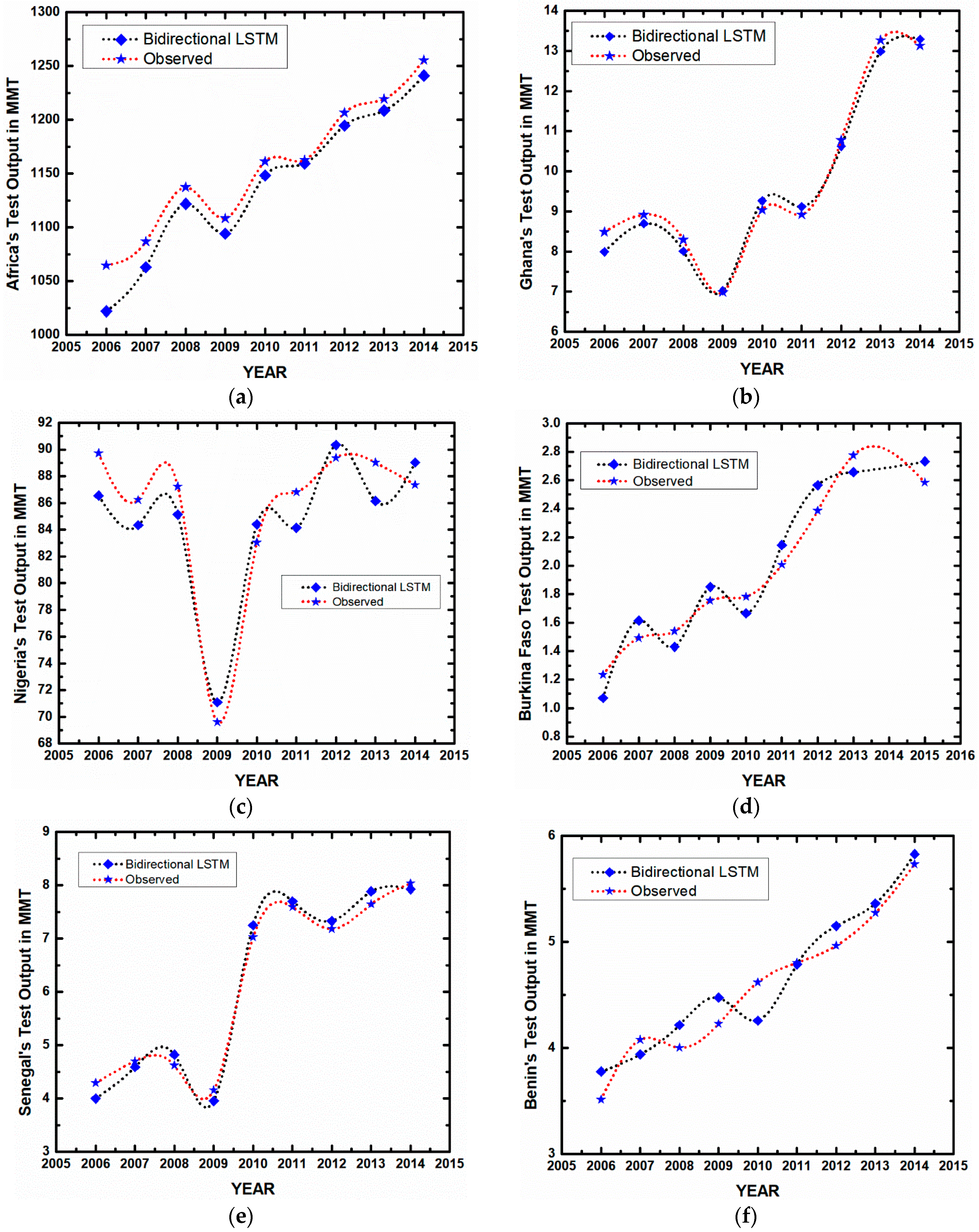
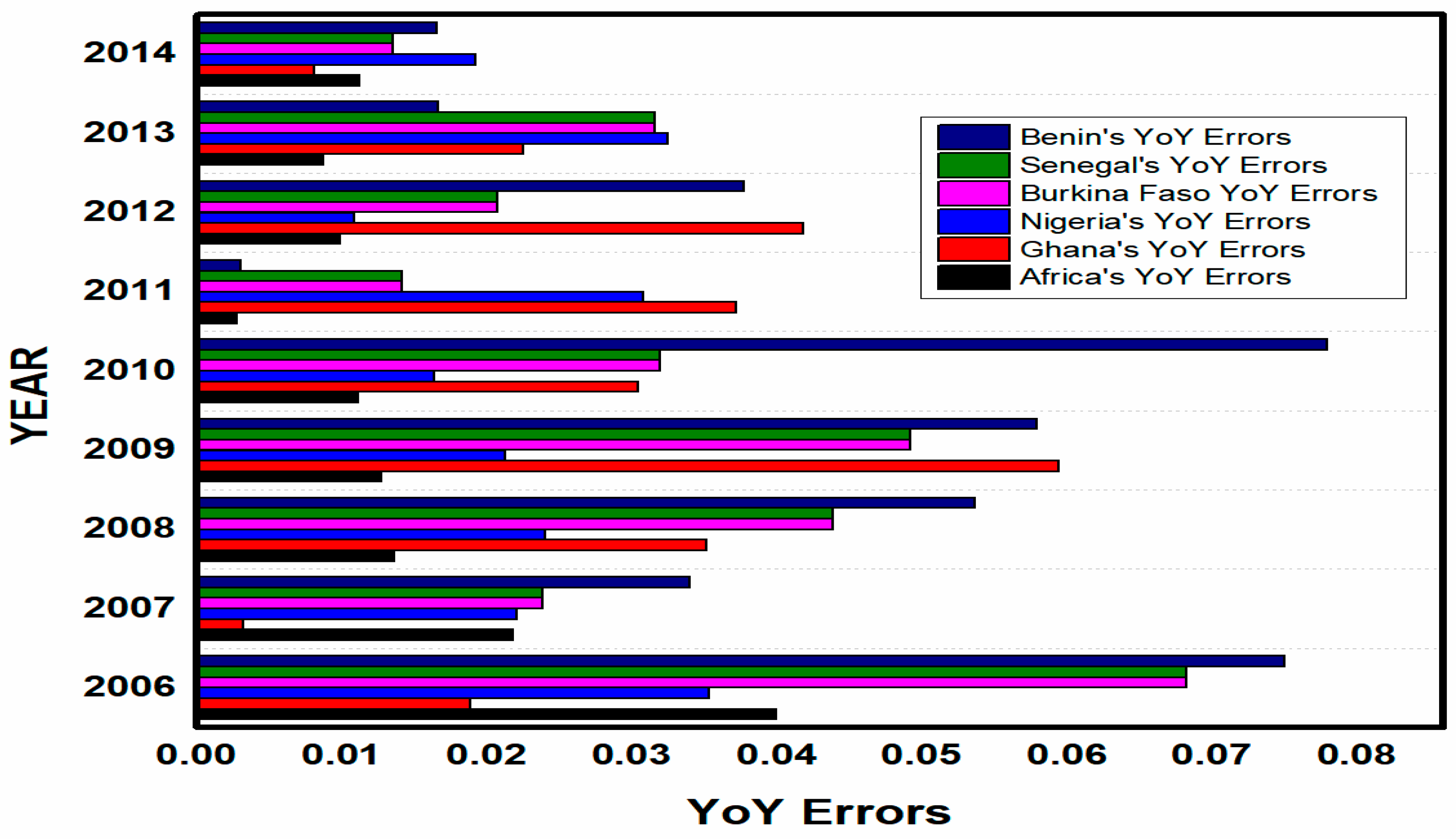
4.1. Testing Stage
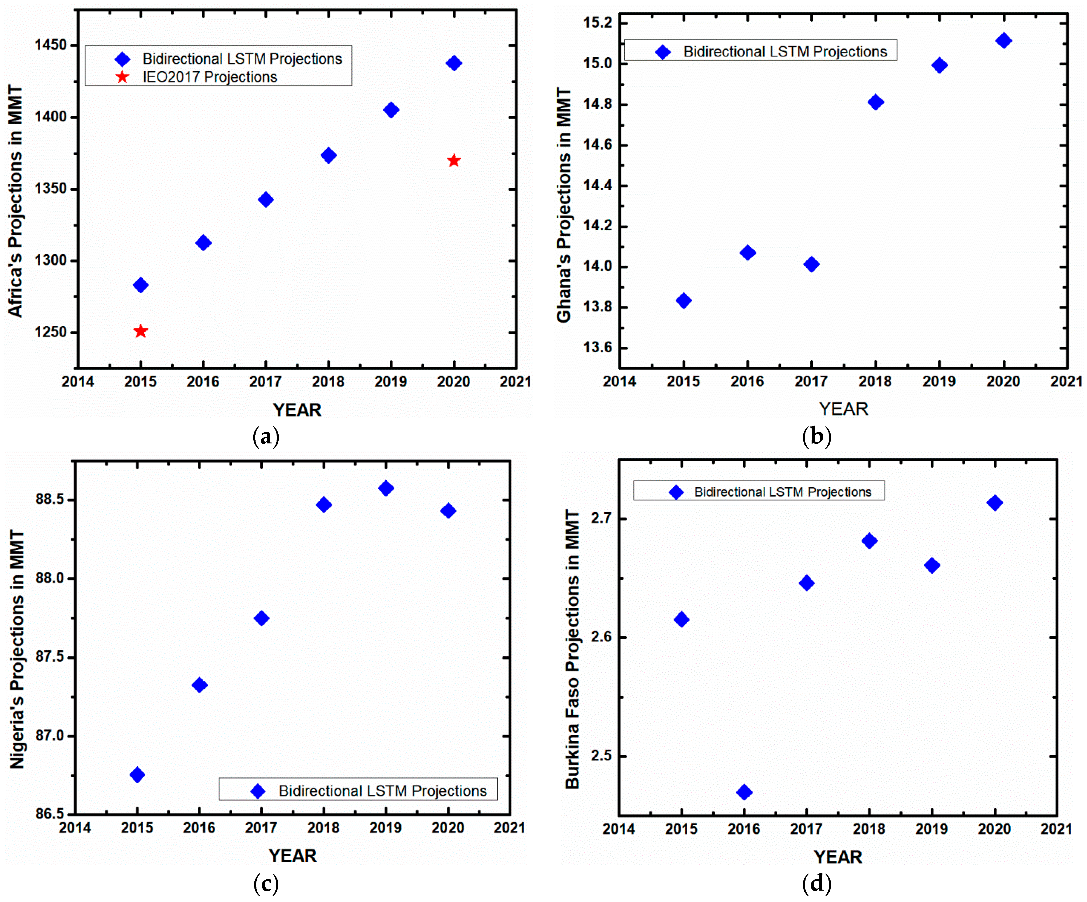
4.2. Forecasting Stage
5. Discussion
6. Conclusions and Policy Recommendations
Author Contributions
Funding
Acknowledgments
Conflicts of Interest
References
- Aye, G.C.; Edoja, P.E. Effect of economic growth on CO2 emission in developing countries: Evidence from a dynamic panel threshold model. Cogent Econ. Financ. 2017, 90, 1–22. [Google Scholar] [CrossRef]
- Huesemann, M.H.; Huesemann, J.A. Will progress in science and technology avert or accelerate global collapse? A critical analysis and policy recommendations. Environ. Dev. Sustain. 2008, 10, 787–825. [Google Scholar] [CrossRef]
- Cherniwchan, J. Economic growth, industrialization, and the environment. Resour. Energy Econ. 2012, 34, 442–467. [Google Scholar] [CrossRef]
- Lu, W. Greenhouse Gas Emissions, Energy Consumption and Economic Growth: A Panel Cointegration Analysis for 16 Asian Countries. Int. J. Environ. Res. Public Heal. 2017, 14, 1436. [Google Scholar] [CrossRef] [PubMed]
- Chandran Govindaraju, V.G.R.; Tang, C.F. The dynamic links between CO2 emissions, economic growth and coal consumption in China and India. Appl. Energy 2013, 104, 310–318. [Google Scholar] [CrossRef]
- Dollar, D.; Kleineberg, T.; Kraay, A. Growth still is good for the poor. Eur. Econ. Rev. 2016, 81, 68–85. [Google Scholar] [CrossRef]
- Di Fonzo, M.; Collen, B.; Mace, G.M. A new method for identifying rapid decline dynamics in wild vertebrate populations. Ecol. Evol. 2013, 3, 2378–2391. [Google Scholar] [CrossRef] [PubMed] [Green Version]
- Mohiuddin, O.; Asumadu-sarkodie, S.; Obaidullah, M. The relationship between carbon dioxide emissions, energy consumption, and GDP: A recent evidence from Pakistan energy consumption, and GDP: A recent evidence. Cogent Eng. 2016, 1, 1–16. [Google Scholar] [CrossRef]
- Höök, M.; Tang, X. Depletion of fossil fuels and anthropogenic climate change—A review. Energy Policy 2013, 52, 797–809. [Google Scholar] [CrossRef] [Green Version]
- Bissey, S.; Jacques, S.; Le Bunetel, J.C. The fuzzy logic method to efficiently optimize electricity consumption in individual housing. Energies 2017, 10, 1701. [Google Scholar] [CrossRef]
- Jayaraman, T. The Paris Agreement on Climate Change: Background, Analysis and Implications. Rev. Agrar. Stud. 2016, 5, 1–31. [Google Scholar]
- He, J.K. Global low-carbon transition and China’s response strategies. Adv. Clim. Chang. Res. 2016, 7, 204–212. [Google Scholar] [CrossRef]
- Reckien, D.; Salvia, M.; Heidrich, O.; Church, J.M.; Pietrapertosa, F.; De Gregorio-Hurtado, S.; D’Alonzo, V.; Foley, A.; Simoes, S.G.; Krkoška Lorencová, E.; et al. How are cities planning to respond to climate change? Assessment of local climate plans from 885 cities in the EU-28. J. Clean. Prod. 2018, 191, 207–219. [Google Scholar] [CrossRef] [Green Version]
- UNFCCC. United Nations Framework Convention on Climate Change Paris Agreement. In Proceedings of the 21st Session of the Conference of the Parties, Paris, France, 30 November–12 December 2015. [Google Scholar]
- Ladislaw, S.; Sullivan, M.L.O.; Raimi, D.; Foss, M.M.; Irwin, S.H. Dominance Energy Abundance Market. 2017. Available online: https://www.oxfordenergy.org/wpcms/wp-content/uploads/2018/01/OEF-111.pdf (accessed on 31 August 2018).
- IPCC. Climate Change 2014: Mitigation of Climate Change; Cambridge University Press: Cambridge, UK, 2014; pp. 527–532. [Google Scholar]
- Wang, C.; Wang, F.; Zhang, X.; Yang, Y.; Su, Y.; Ye, Y.; Zhang, H. Examining the driving factors of energy related carbon emissions using the extended STIRPAT model based on IPAT identity in Xinjiang. Renew. Sustain. Energy Rev. 2017, 67, 51–61. [Google Scholar] [CrossRef]
- Cho, C.-H.; Chu, Y.-P.; Yang, H.-Y. An Environment Kuznets Curve for GHG Emissions: A Panel Cointegration Analysis. Energy Sources Part B Econ. Plan. Policy 2014, 9, 120–129. [Google Scholar] [CrossRef]
- Giovanis, E. Environmental Kuznets curve: Evidence from the British Household Panel Survey. Econ. Model. 2013, 30, 602–611. [Google Scholar] [CrossRef]
- Tang, C.F.; Tan, B.W.; Ozturk, I. Energy consumption and economic growth in Vietnam. Renew. Sustain. Energy Rev. 2016, 54, 1506–1514. [Google Scholar] [CrossRef]
- Komal, R.; Abbas, F. Linking financial development, economic growth and energy consumption in Pakistan. Renew. Sustain. Energy Rev. 2015, 44, 211–220. [Google Scholar] [CrossRef]
- Cowan, W.N.; Chang, T.; Inglesi-Lotz, R.; Gupta, R. The nexus of electricity consumption, economic growth and CO2 emissions in the BRICS countries. Energy Policy 2014, 66, 359–368. [Google Scholar] [CrossRef]
- Asongu, S.; El Montasser, G.; Toumi, H. Testing the relationships between energy consumption, CO2 emissions, and economic growth in 24 African countries: A panel ARDL approach. Environ. Sci. Pollut. Res. 2016, 23, 6563–6573. [Google Scholar] [CrossRef] [PubMed]
- Abid, M. The close relationship between informal economic growth and carbon emissions in Tunisia since 1980: The (ir)relevance of structural breaks. Sustain. Cities Soc. 2015, 15, 11–21. [Google Scholar] [CrossRef]
- Esso, L.J.; Keho, Y. Energy consumption, economic growth and carbon emissions: Cointegration and causality evidence from selected African countries. Energy 2016, 114, 492–497. [Google Scholar] [CrossRef]
- Ameyaw, B.; Yao, L. Sectoral Energy Demand Forecasting under an Assumption-Free Data-Driven Technique. Sustainability 2018, 10, 2348. [Google Scholar] [CrossRef]
- Hu, Y.C.; Jiang, P. Forecasting energy demand using neural-network-based grey residual modification models. J. Oper. Res. Soc. 2017, 68, 556–565. [Google Scholar] [CrossRef]
- Abdel-Aal, R.E. Univariate modeling and forecasting of monthly energy demand time series using abductive and neural networks. Comput. Ind. Eng. 2008, 54, 903–917. [Google Scholar] [CrossRef]
- Hamzaçebi, C. Primary energy sources planning based on demand forecasting: The case of Turkey. J. Energy Southern Afr. 2016, 27, 2–10. [Google Scholar] [CrossRef]
- WIND. Wind-Financial Terminal News. Available online: http://www.wind.com.cn/en/wft.html (accessed on 15 July 2018).
- World Bank. World Development Indicators 2015; World Bank: Washington, DC, USA, 2015; ISBN 9780821373866. [Google Scholar]
- Canadell, J.G.; Raupach, M.R.; Houghton, R. A Anthropogenic CO2 Emissions in Africa. Biogeosciences 2009, 6, 463–468. [Google Scholar] [CrossRef]
- Marchal, V.; Dellink, R.; Van Vuuren, D.; Clapp, C.; Château, J.; Lanzi, E.; Magné, B.; Van Vliet, J. OECD Environmental Outlook to 2050: Climate Change Chapter. 2011. Available online: https://www.oecd.org/env/cc/49082173.pdf (accessed on 18 July 2018).
- Meng, J.; Mi, Z.; Guan, D.; Li, J.; Tao, S.; Li, Y.; Feng, K.; Liu, J.; Liu, Z.; Wang, X.; et al. The rise of South-South trade and its effect on global CO2 emissions. Nat. Commun. 2018. [Google Scholar] [CrossRef] [PubMed]
- Davis, S.J.; Caldeira, K. Consumption-based accounting of CO2 emissions. Proc. Natl. Acad. Sci. USA 2010. [Google Scholar] [CrossRef] [PubMed]
- Maestas, N.; Mullen, K.J.; Powell, D. The Effect of Population Aging on Economic Growth, the Labor Force and Productivity. 2016. Available online: http://www.nber.org/papers/w22452 (accessed on 18 July 2018).[Green Version]
- Ugochukwu, U.S.; Chinyere, U.P. The Impact of Capital Formation on the Growth of Nigerian Economy. Res. J. Financ. Account. 2013, 4, 36–43. [Google Scholar]
- Cobb, C.; Douglas, P. A Theory of Production. Am. Econ. Rev. 1928, 18, 139–165. [Google Scholar]
- Ameyaw, B.; Oppong, A.; Abruquah, L.A.; Ashalley, E. Causality Nexus of Electricity Consumption and Economic Growth: An Empirical Evidence from Ghana. Open J. Bus. Manag. 2017, 5, 1–10. [Google Scholar] [CrossRef]
- Karekezi, S.; Kithyoma, W. Renewable energy development. In Proceedings of the Workshop for African Energy Experts on Operationalising the NEPAD Energy Initiative, Dakar, Senegal, 2–4 June 2003. [Google Scholar]
- Pesaran, M.H. General Diagnostic Tests for Cross Section Dependence in Panels. Available online: https://papers.ssrn.com/sol3/papers.cfm?abstract_id=572504 (accessed on 18 July 2018).
- Breusch, T.S.; Pagan, A.R. The Lagrange Multiplier Test and its Applications to Model Specification in Econometrics. Rev. Econ. Stud. 1980, 47, 239. [Google Scholar] [CrossRef]
- Im, K.S.; Pesaran, M.H.; Shin, Y. Testing for Seasonal Unit Roots in Heterogeneous Panels. J. Econom. 2003, 115, 53–74. [Google Scholar] [CrossRef]
- Levin, A.; Lin, C.F.; Chu, C.S.J. Unit root tests in panel data: Asymptotic and finite-sample properties. J. Econom. 2002, 108, 1–24. [Google Scholar] [CrossRef]
- Pedroni, P. Panel Cointegration: Asymptotic and Finite Sample Properties of Pooled Time Series Tests with an Application to the PPP hypothesis. Econom. Theory 2004, 20, 597–625. [Google Scholar] [CrossRef]
- Apergis, N.; Payne, J.E. A time varying coefficient approach to the renewable and non-renewable electricity consumption-growth nexus: Evidence from a panel of emerging market economies. Energy Sources Part B Econ. Plan. Policy 2014, 9, 101–107. [Google Scholar] [CrossRef]
- Apergis, N.; Payne, J.E. Renewable energy consumption and economic growth: Evidence from a panel of OECD countries. Energy Policy 2010, 38, 656–660. [Google Scholar] [CrossRef]
- Engle, R.F.; Granger, C.W.J. Co-Integration and Error Correction: Representation, Estimation, and Testing. Econometrica 1987, 55, 251. [Google Scholar] [CrossRef]
- Granger, C.W.J. Investigating Causal Relations by Econometric Models and Cross-spectral Methods. Econometrica 1969, 37, 424. [Google Scholar] [CrossRef]
- International Energy Agency-U.S. Unit Converter. 2016. Available online: https://ww.iea.org/statistics/resources/unit converter/ (accessed on 15 July 2018).
- U.S. Energy Information Administration. International Energy Outlook 2010; Department of Energy: Washington, DC, USA, 2010.
- U.S. Energy Information Administration. International Energy Outlook 2011; Department of Energy: Washington, DC, USA, 2011.
- U.S. Energy Information Administration. International Energy Outlook 2013; Department of Energy: Washington, DC, USA, 2013.
- Barone, A.V.M.; Helcl, J.; Sennrich, R.; Haddow, B.; Birch, A. Deep Architectures for Neural Machine Translation. In Proceedings of the Second Conference on Machine Translation, Copenhagen, Denmark, 7–8 September 2017; pp. 99–107. [Google Scholar]
- Hou, L.; Samaras, D.; Kurc, T.; Gao, Y.; Saltz, J. ConvNets with Smooth Adaptive Activation Functions for Regression. In Proceedings of the 20th International Conference on Artificial Intelligence and Statistics, Fort Lauderdale, FL, USA, 20–22 April 2017; pp. 430–439. [Google Scholar]
- Helmbold, D.P.; Long, P.M. Surprising properties of dropout in deep networks. J. Mach. Learn. Res. 2016, 65, 1–24. [Google Scholar]
- U.S. Energy Information Administration International Energy Outlook 2017. Available online: www.eia.gov/forecasts/ieo/pdf/0484(2016).pdf (accessed on 18 July 2018).
- Palamalai, S.; Siddanth, I.; Prakasam, K. Relationship between Energy Consumption, CO2 Emissions, Economic Growth and Trade in India. J. Econ. Financ. Stud. 2015, 1, 1–17. [Google Scholar] [CrossRef]
- Lim, K.-M.; Lim, S.-Y.; Yoo, S.-H. Oil Consumption, CO2 Emission, and Economic Growth: Evidence from the Philippines. Sustainability 2014, 6, 967–979. [Google Scholar] [CrossRef]
- Kasperowicz, R. Economic growth and CO2 emissions: The ECM analysis. J. Int. Stud. 2015, 8, 91–98. [Google Scholar] [CrossRef]
- Anis, O. CO2 Emissions, Energy Consumption and Economic Growth Nexus in MENA countries: Evidence from Simultaneous Equation Models. Energy Econ. 2013, 40, 657–664. [Google Scholar]
- Wang, Z.; Wang, J.; He, D. Transit Policies and Potential CO2 Emission Impacts—Some Insights from China’ s Transit Priority Policies in Recent Years. Transp. Res. Board. 2012, 19, 1–14. [Google Scholar] [CrossRef]
- Gu, B.; Tan, X.; Zeng, Y.; Mu, Z. CO2 Emission Reduction Potential in China’s Electricity Sector: Scenario Analysis Based on LMDI Decomposition. Energy Procedia 2015, 75, 2436–2447. [Google Scholar] [CrossRef]
- Allali, M.; Tamali, M.; Rahli, M. The Impact of CO2 Emission on Output in Algeria. Energy Procedia 2015, 74, 234–242. [Google Scholar] [CrossRef]
- Du, S.; Zhu, L.; Liang, L.; Ma, F. Emission-dependent supply chain and environment-policy-making in the “cap-and-trade” system. Energy Policy 2013, 57, 61–67. [Google Scholar] [CrossRef]


| Variables | Definition | Data Source | Unit |
|---|---|---|---|
| CO2 | Carbon dioxide emissions | WIND [30] | 1000 tons |
| GDPC | Gross domestic product per capita | WDI [31] | Constant 2010 US$ |
| LF | Labor force | WDI [31] | Total Labor force |
| GFCF | Gross fixed capital formation | WDI [31] | Percentage (%) of GDP |
| Cross-Sectional Dependence Test | Pesaran’s Test | p-Value |
|---|---|---|
| Pesaran’s Test | 3.6849 | 0.0253 y |
| Form | Variables | L.L&C | IPS | ADF | PP-Fisher | Conclusions |
|---|---|---|---|---|---|---|
| Level | lnCO2 | 0.7532 (0.7368) | 0.3564 (0.5983) | 0.7191 (0.6037) | 1.3899 (0.3784) | Non-stationary |
| lnGDPC | 0.6891 (0.6582) | 1.9332 (0.9173) | 0.05728 (0.9428) | 0.0482 (0.9682) | Non-stationary | |
| lnLF | −1.2382 (0.2920) | −0.3873 (0.3649) | 1.8320 (0.3289) | 1.4897 (0.4928) | Non-stationary | |
| lnGFCF | −0.5803 (0.1893) | 0.2894 (0.3702) | 1.8739 (0.3492) | 1.0478 (0.6397) | Non-stationary | |
| First Difference | ΔlnCO2 | −1.2513 (0.0392) y | −0.9527 (0.0402) y | 4.6891 (0.0447) y | 6.8024 (0.469) y | Stationary |
| ΔlnGDPC | −2.5856 (0.0005) x | −1.9274 (0.0264) y | 6.9357 (0.0317) y | 10.6134 (0.0021) x | Stationary | |
| ΔlnLF | −1.8397 (0.0001) x | −1.3492 (0.0017) x | 7.9582 (0.0021) x | 9.5983 (0.0004) x | Stationary | |
| ΔlnGFCF | −0.4294 (0.0203) y | −0.1793 (0.0217) y | 5.8937 (0.0289) y | 7.6743 (0.0185) y | Stationary |
| Method | Test Statistics | Value | Probability |
|---|---|---|---|
| Pedroni | Panel v-Statistics | −1.4684 | 0.0294 y |
| Panel rho-Statistics | −1.1490 | 0.0379 y | |
| Panel PP-Statistics | −5.8294 | 0.0071 x | |
| Panel ADF-Statistics | −1.7236 | 0.0014 x | |
| Group rho-Statistics | −1.6873 | 0.0117 y | |
| Group PP-Statistics | −7.5832 | 0.0000 x | |
| Group ADF-Statistics | −1.3848 | 0.0019 x |
| Null Hypothesis | Ghana | Nigeria | Burkina-Faso | Senegal | Benin |
|---|---|---|---|---|---|
| lnGDPC does not Granger cause lnCO2 | 8.9482 (0.0029) x | 12.6892 (0.0021) x | 4.7492 (0.0278) y | 5.0254 (0.0178) y | 4.1394 (0.0278) x |
| lnCO2 does not Granger cause lnGDPC | 1.1274 (0.1585) | 1.1946 (0.2742) | 0.2172 (0.3673) | 0.1734 (0.1949) | 0.0978 (0.4822) |
| lnLF does not Granger cause lnCO2 | 9.7839 (0.0382) y | 11.2674 (0.0288) y | 5.0269 (0.0458) y | 5.9426 (0.0378) y | 3.4980 (0.0279) y |
| lnCO2 does not Granger cause lnLF | 2.6542 (0.1178) | 2.9459 (0.1830) | 1.9894 (0.7595) | 2.1387 (0.8427) | 1.3738 (0.6921) |
| lnGFCF does not Granger cause lnCO2 | 4.5921 (0.6821) | 5.4298 (0.8468) | 3.0129 (0.6193) | 3.7342 (0.7742) | 2.1617 (0.4782) |
| lnCO2 does not Granger cause lnGFCF | 1.5967 (0.3247) | 1.9678 (0.3957) | 1.1204 (0.2895) | 1.3849 (0.3076) | 1.0068 (0.2154) |
| IEO2010 (Africa in MMT) | |||||
| 2006 | 2007 | ||||
| Observed | BiLSTM | IEO Projection | Observed | BiLSTM | IEO Projection |
| 1064.547 | (1021.971) | 988 | 1086.893 | (1063.184) | 1011 |
| YoY Error | |||||
| 0.040 | 0.072 | 0.022 | 0.070 | ||
| IEO2013 (Africa in MMT) | |||||
| 2009 | 2010 | ||||
| Observed | BiLSTM | IEO Projection | Observed | BiLSTM | IEO Projection |
| 1108.286 | (1094.129) | 1047 | 1161.128 | (1148.208) | 1070 |
| YoY Error | |||||
| 0.013 | 0.055 | 0.011 | 0.078 | ||
| IEO2011 (Africa in MMT) | |||||
| 2011 | 2012 | ||||
| Observed | BiLSTM | IEO Projection | Observed | BiLSTM | IEO Projection |
| 1162.475 | (1159.231) | 1120 | 1206.576 | (1194.608) | 1184 |
| YoY Error | |||||
| 0.003 | 0.040 | 0.010 | 0.019 | ||
© 2018 by the authors. Licensee MDPI, Basel, Switzerland. This article is an open access article distributed under the terms and conditions of the Creative Commons Attribution (CC BY) license (http://creativecommons.org/licenses/by/4.0/).
Share and Cite
Ameyaw, B.; Yao, L. Analyzing the Impact of GDP on CO2 Emissions and Forecasting Africa’s Total CO2 Emissions with Non-Assumption Driven Bidirectional Long Short-Term Memory. Sustainability 2018, 10, 3110. https://doi.org/10.3390/su10093110
Ameyaw B, Yao L. Analyzing the Impact of GDP on CO2 Emissions and Forecasting Africa’s Total CO2 Emissions with Non-Assumption Driven Bidirectional Long Short-Term Memory. Sustainability. 2018; 10(9):3110. https://doi.org/10.3390/su10093110
Chicago/Turabian StyleAmeyaw, Bismark, and Li Yao. 2018. "Analyzing the Impact of GDP on CO2 Emissions and Forecasting Africa’s Total CO2 Emissions with Non-Assumption Driven Bidirectional Long Short-Term Memory" Sustainability 10, no. 9: 3110. https://doi.org/10.3390/su10093110
APA StyleAmeyaw, B., & Yao, L. (2018). Analyzing the Impact of GDP on CO2 Emissions and Forecasting Africa’s Total CO2 Emissions with Non-Assumption Driven Bidirectional Long Short-Term Memory. Sustainability, 10(9), 3110. https://doi.org/10.3390/su10093110