Activity Based Costing for Wastewater Treatment and Reuse under Uncertainty: A Fuzzy Approach

Abstract

The objective of this article is to present a methodology for computing and allocating wastewater recuperation costs using an Activity-Based Costing (ABC) methodology. One of the most critical problems in modelling those costs is the limited information and the subjectivity used to represent some of the cost’s elements (e.g., values, drivers, among others). Thus, a fuzzy ABC approach is incorporated into the methodology to overcome those limitations. The application of this methodology aims at providing an alternative procedure to allocating the costs related to wastewater management activities to products. To validate the proposed methodology and illustrate its utility, a case study using data from a bus assembly plant is provided. Part of the wastewater produced is coming from a surface treatment installation which, after a recovery process, reuse part of the same water in a closed loop circuit. Using the proposed Fuzzy ABC methodology, the costs (including uncertainty) of the surface treatment and water treatment activities can be appropriately allocated to the products that generate those activities and that waste.

1. Introduction

The environmental issue must be considered a top priority challenge that companies are facing and will continue to face in the upcoming years [1]. Organizations are under pressure to adopt environmental policies and incorporate them into strategic planning as a routine [2]. Nowadays, the legal restrictions and social perception are becoming more stringent. Clients (stakeholders) are increasingly demanding and looking for products and processes that are less harmful to the environment. Thus, the correct evaluation of the environmental factors is fundamental for the survival of companies, both in the medium and long-term, in developed and developing countries [3,4,5,6].

The environmental costs include all the costs of the resources (expenses) used by the activities developed for the purpose of caring for and/or recovering the environment. The term environmental cost, even today, is a term of difficult conceptualization since the literature does not present a clear and objective definition of what is considered an environmental cost. The first difficulty encountered in managing environmental costs is the fact that many of them are considered intangible; and even more, practically all companies that consider the existence of these costs treat them as an externality. The internalization of environmental costs may lead the organization towards a process of generating lower impacts and, to more efficient and effective environmental management [7].

The main sustainability strategies should aim to [8]:

• Reduce to the minimum possible, if not eliminate, the production of polluting waste.
• Maximize productivity with increasing sustainability, and
• Implement and maintain effective environmental management systems at the lowest possible cost.

Therefore, cost control will reflect the level of failures (environmental) occurred and the volume of expenditures necessary to avoid and/or reduce such failures [9]. Such expenditures may be considered as capital investments or greater quantities of inputs in the operational process. Environmental cost management must be considered as an important information item for the organization, contributing to leverage its productivity levels, generating more value for shareholders and increasing sustainability.

Costs of an environmental nature can be subdivided into [9,10,11,12]:

• Costs of environmental control
• Environmental Costs of Prevention
• Environmental Assessment Costs
• Costs of environmental control failures
• Mitigation costs of internal faults
• Costs Mitigation of external faults
• Costs of environmental control

Among the expenses that can be considered as environmental costs, we can cite the following examples [13]:

• Investments in anti-pollution technologies;
• Specific materials intended for environmental protection, preservation and recovery;
• Hours of labour consumed in effluent treatment stations.

Therefore, the environmental issue should be seen as a multidisciplinary issue and, to be appropriately addressed, it needs to be analysed globally. The treatment of wastewater and its further reuse is an essential part of the rationalization of water and a critical factor in environmental management [14,15].

Therefore, actions related to the improvement of wastewater treatment and reuse should be undertaken in terms of improving economic and environmental sustainability. Within the perspective of severe climate change, the practices of wastewater recovery and reuse do not seem an option, but an obligation [16]. The reuse of industrial wastewater is an inseparable part of the concept of sustainable production. Following the agricultural sector, the industrial sector is one of the largest users of water for development, consuming almost 20% of global water withdrawals [17]. The metal coating industry is one of the industries that consumes the largest amounts of water. On average, developed countries treat about 70% of the wastewater they generate. On the other hand, in developing countries, only 8% of industrial and municipal wastewater undergoes treatment of any kind [18]. Therefore, globally, over 80% of wastewater is released to the environment without adequate treatment [19,20]. One estimate suggests that the volumes of industrial wastewater will double by 2025 [21,22]. The data also show that manufacturing is the highest generator of wastewater among the main industrial sectors [23,24].

As already mentioned, there is a tendency in some organizations to consider many of the costs related to wastewater recovery and reuse as indirect costs [25,26,27,28,29]. That assumption leads organizations to allocate them using some subjective (and imperfect) criterion or rate. This is due, to a large extent, to the uncertainty that exists when calculating the values of environmental expenditures and in selecting the most appropriate cost drivers [30,31].

Activity-based costing (ABC) has been widely used in a great variety of scenarios where indirect costs have to be measured and correctly allocated to product costs. However, in circumstances where there are important degrees of uncertainty, ABC is unable to efficiently incorporate any uncertain value and possible variability [32]. When data is uncertain, the outputs of the ABC method cannot be considered as reliable, and many procedures based on interviews, judgement and simulation become necessary [33,34]. By doing this, the estimates are very likely to be considered imprecise and, at last, useless [35].

Zadeh [36] proposed the fuzzy theory, which is based on the rationality of uncertainty due to factors such as imprecision and vagueness. Nachtmann and Needy [37] concluded that, based on a comparative cost/benefit analysis, Monte Carlo simulation and fuzzy set theory are superior to interval mathematics as methods for handling inherent data uncertainty and imprecision into ABC models. In recent years, techniques based on fuzzy numbers have emerged as an excellent tool to manage uncertainty in models for calculating costs [37].

Given the necessity to allocate the cost related to environmental activities correctly, using precise information and within uncertain scenarios, this paper proposes the use of an activity-based costing technique using fuzzy numbers for a wastewater treatment plant from a metallic parts coating line in a bus body assembler.

The next sections are devoted to discussing the need for an appropriate wastewater treatment cost allocation method; then, we will analyse how activity-based costing can contribute to higher accuracy in the process of allocating those costs to object costs. In addition, the use of fuzzy numbers is included in such discussion. Next, a novel matrix model, based on fuzzy activity-based costing, is presented to compute such costs. The proposal is followed by a validation example constructed from a real case application. Finally, results analysis and discussion are provided.

2. Activity-Based Costing (ABC)

Conventional costing systems assume that the products are the cause of the costs. Therefore, the product unit is considered the central point of the costing system. From that, the costs are allocated to the products either directly or indirectly, according to whether the costs can be economically traced to the cost object or not. These systems use measures related to the volume of production to allocate indirect costs (overhead) to the cost objects, including labor hours or the amount of raw material used. Such costing systems show an acceptable precision in the case in which indirect activities are generated based on the volume produced, such as the cost of electric power which is a function of machine hours. However, some costs cannot be appropriately allocated to object costs if the production volume is used as the only cost driver.

The problem of the correct allocation of environmental costs becomes crucial as its importance and amounts have increased in recent years. Managers are provided with useful information to lead actions pointed to obtain better environmental performance, applying the correct allocation of these costs. We can mention, for example, the prescription of better anti-pollution measures, as well as the control or mitigation of the damages caused by specific industrial processes, with the subsequent evaluation of the impacts that this may cause on the costs of a product.

Traditionally, environmental costs have been treated as indirect costs (overheads) [38]. These costs are not allocated to specific processes, products or facilities, but they are generally managed through one of the following methods:

(1)

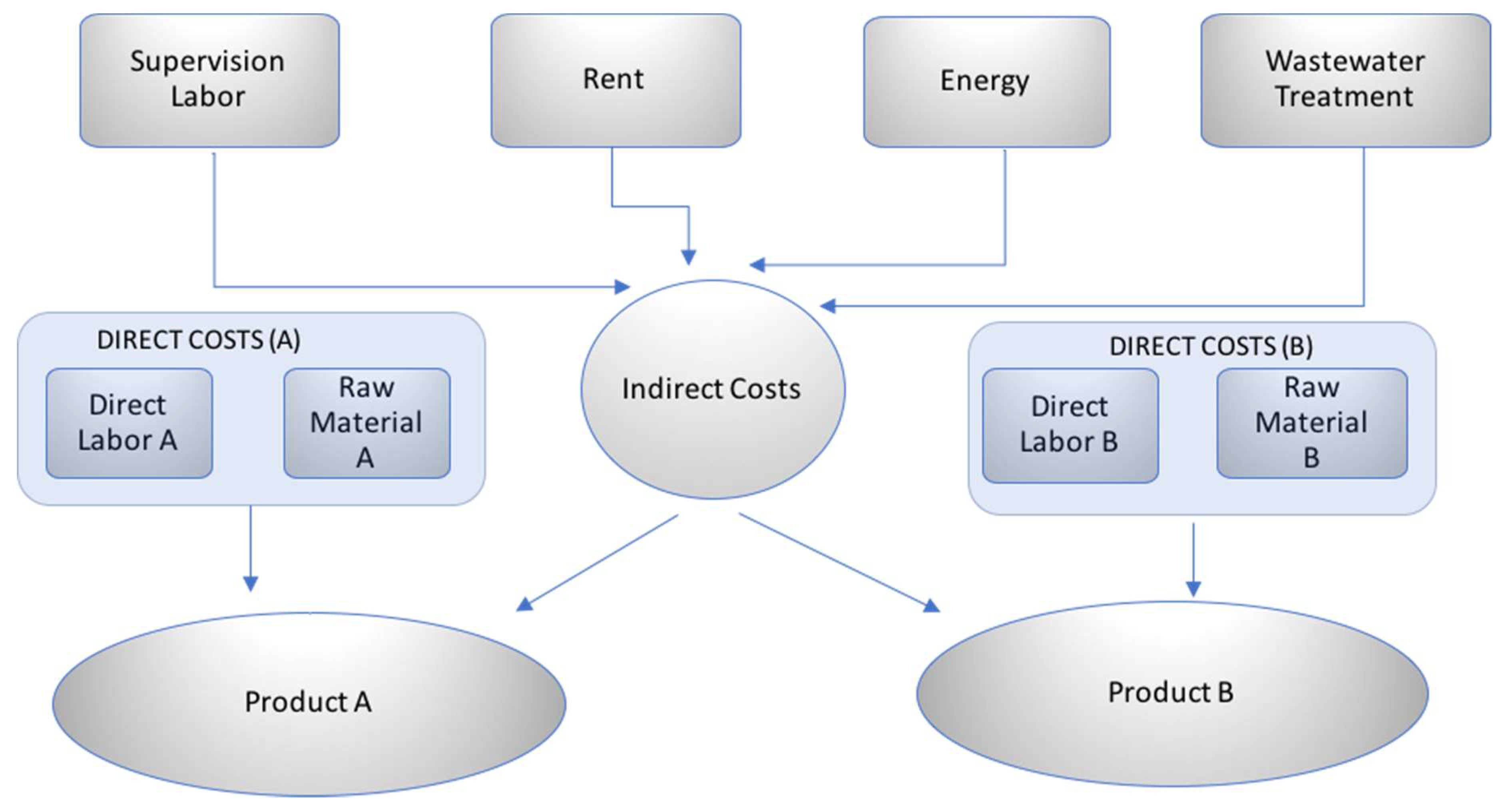
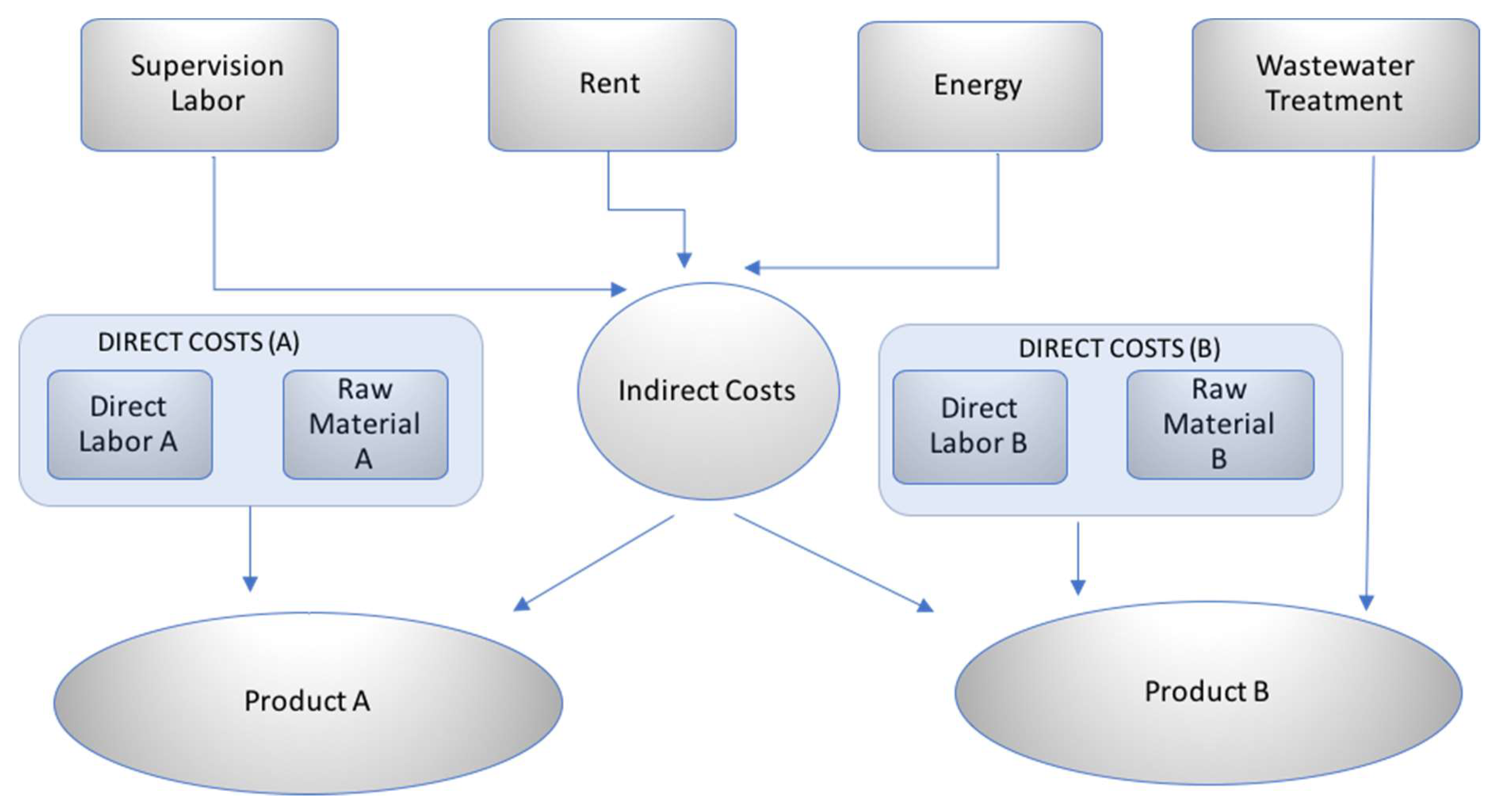
They are allocated based on some simple criteria of allocation to the products.

(2)

They are accumulated in a costs pool, which means they are not allocated to any specific product, and they are treated as fixed costs or overhead.

If the indirect costs are incorrectly allocated, a given product may receive a greater share of indirect costs than the correct one [27]. Meanwhile, a lower share of costs may be allocated to another product, producing imbalances that will affect the decision-making process. This imbalance will harm, for instance, the correct definition of products’ prices, their margin of contribution and finally affecting the long-term profitability of the organization.

This situation can be illustrated through a simple example. Consider in Figure 1, a traditional cost system, where the environmental costs and other indirect costs are allocated to two different products (A and B), using as a basis for allocation, hours of direct labour (MOD) and raw material (RM). Suppose that product B is the exclusive cause of the effluents which are treated by the company. The traditional costing system may cause an imbalance in the allocation of environmental costs, since part of those costs will be allocated to the product A, considering that such a product does not contribute to generating effluents of any kind.

Figure 2 exemplifies the new vision of the cost system. Such a vision treats environmental costs in a more balanced way, allocating them only to product B. This is done by extracting from the set of indirect costs all the costs related to the effluents treatment.

When one is performing cost calculation and analysis, there may be some key information elements about which uncertainty exists. Different authors have addressed the uncertainty in cost evaluations and data estimation. Many of them classify uncertainty in two main classes: epistemic and aleatory. Yee Mey Goh [39] presented a review of the uncertainty classification in engineering literature. According to the American Institute of Chemical Engineers (AIChE), five categories of costs are established. Each category is considered increasingly difficult to quantify than the previous ones:

• Direct Costs (Capital Investments, Recurring and non-recurring costs)
• Indirect Costs (operating and maintenance, recurring and non-recurring)
• Contingent (future scenarios)
• Intangible (Customer loyalty, working morale and performance)
• External Costs (Societal costs)

On this, it is worth mentioning that the higher the cost category considered, the more uncertain the estimated cost values will be. The activity-based costing system divides the organization into processes and these processes into activities. An activity represents what the company does, the time it spends doing it, and the product obtained. Activity costing identifies the activities performed on the cost object and determines its costs and benefits. When comparing the approaches of both models, it is appreciated that the traditional model allocates resources to cost objects directly. Whereas, the activity-based costing model allocates the costs of the resources to the activities carried out by the organization to produce the cost objects and then allocate the costs of the activities to the cost objects (Figure 3). Therefore, it is crucial for the correct selection of the activity drivers. For example, the cost of inspecting a unitary piece of each lot produced will be related to the number of lots and not to the number of pieces, the cost of the processing purchase orders will be related to the number of orders and not to the number of products ordered.

In comparison to traditional costing methods, ABC uses a higher number of allocation bases to identify, in monetary terms, how the activities consume resources for their execution. Using specific cost drivers for each activity, the ABC allows calculating, with a high level of precision, the number of resources that are consumed by each cost object. For the implementation of ABC costing, the following steps should be considered:

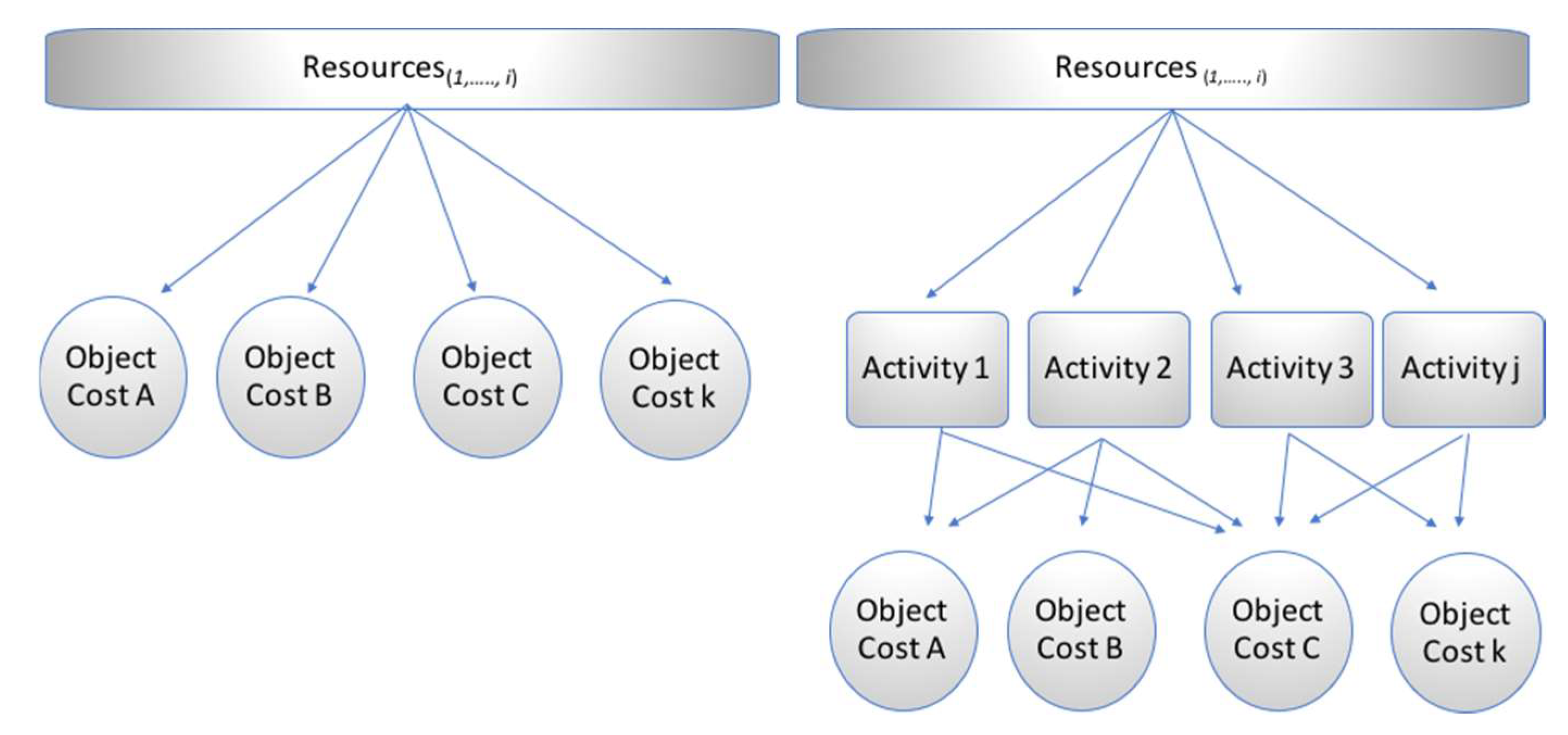
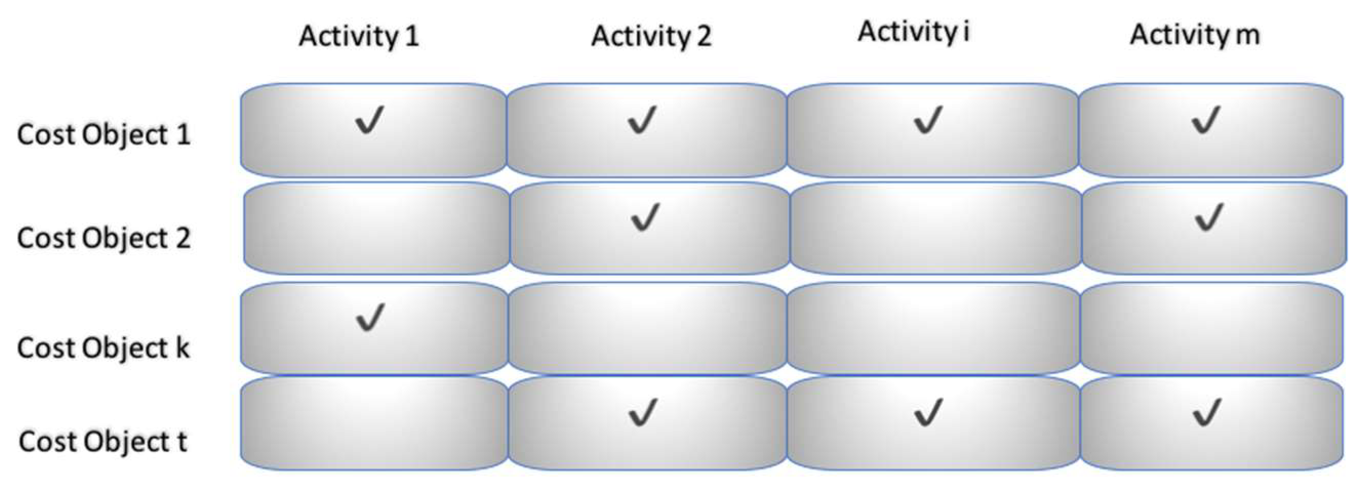
• Identification of activities (activity mapping)
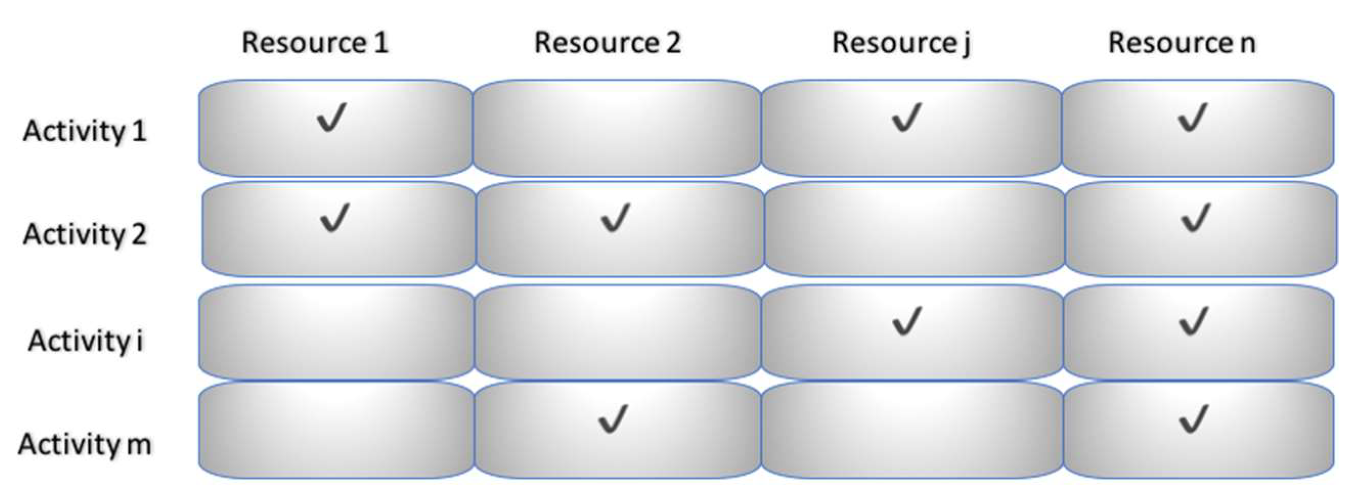
• Listing the resources consumed by each one of the activities.
• List the resources (and their costs) which are consumed by the activities listed in the previous step.
• Determination of the first and second level cost drivers.
• Determination of the activities’ costs.
• Determination of the cost of the costs objects.

Afonso and Paisana [40] proposed a novel representation of the ABC algorithm based on matrix multiplication. In such a representation, data relating resources, activities, cost objects and a series of costs drivers are represented using matrices and vectors as is shown in Figure 4 and Figure 5. The symbol √ means that a relationship exists between a resource and an activity or between an activity and a cost object.

In the first allocation phase, the calculation of cost per activity, the resource-activity matrix, which contains r_ij terms which represent the proportion of the resource driver j that is related to activity i, is multiplied by the resource matrix whose terms r_j represent the total amount of the resource j expended during the period under analysis. That multiplication results in the so-called Activities Matrix, where the term a_i represents the amount of cost allocated for activity i.

[r_ij][r_j] = [a_i]

(1)

Note that in the resource-activity matrix, its elements represent the proportion of the resource driver j that is related to activity i. That proportion is obtained as the ratio between the resource driver j related to activity i (r_ij) and the total amount of the resource driver j (r_j). Then, the cost allocated to each activity will be obtained by:

$$a_i={\displaystyle \sum }_{j=1}^n{r}_{ij}\times r_j$$

(2)

In the second allocation phase, the cost calculation per cost object will be carried out by multiplying the activity product matrix (a_ki) by the vector column of the activity costs (a_i) obtaining the so-called cost object matrix (p_k):

[a_ki] [a_i] = [p_k]

(3)

Considering the Activity-Product matrix, each element a_ki is the proportion of the activity driver related to product k. That proportion is obtained by computing the ratio between the activity-driver i, related to product k (a_ki) and the total amount of the activity-driver i (a_i). Then, the cost imputed to each activity will be obtained by:

$$p_i={\displaystyle \sum }_{i=1}^m{a}_{ki}\times a_i$$

(4)

In summary, the cost object matrix can be obtained in just one step as shown below:

[a_kj] [r_ij][r_j] = [p_k]

(5)

A fuzzy extension of the ABC is proposed to overcome the aforementioned uncertainty influence present during the costing procedure. In the next section, we describe the fuzzy ABC technique proposed. Besides, an example of the application of the proposed technique in a surface treatment plant is presented.

3. Proposed Model

When uncertainties in the input are totally or partially unknown and random, they are usually represented by probability density functions. Many times, there is an absence of historical data for one or more input parameters, in those cases, subjective assessments for the likely values of that variables have to be elicited from experts. It is well accepted that to represent these subjective assessments, fuzzy numbers are used [41]. A critical assessment of the fuzzy number methodology as a potential substitute for probabilistic simulation models was carried out by Byrne [41].

When the decision-maker faces a complex and uncertain problem, and he/she expresses his/her judgments as uncertain ratios [42,43,44]; several authors have addressed this uncertainty using fuzzy numbers [45]. A fuzzy number reveals the meaning of expressions such as ‘about x’. That meaning is represented using a membership function. Such a function could be defined using a triangular number, (a1, a2, a3). The values of the triangular number are used to represent the output of the fuzzy membership function as shown in Equation (6) and Figure 6.

$$\mathsf{\mu }\left(\mathrm{x}\right)=\{\begin{array}{cc}1& x=a_2\\ \frac{x-a_1}{a_2-a_1}& a_1\le x<a_2\\ \frac{a_3-x}{a_3-a_2}& a_2<x\le a_3\\ 0& otherwise\end{array}$$

(6)

To operate with triangular numbers, a set of operations is needed. Next, a brief description about addition, multiplication and division of triangular numbers is given. The fuzzy operators were adapted from Reference [46] and are based on the extent analysis with the use of triangular fuzzy numbers [47].

Let A and B be two triangular fuzzy numbers, with their parameters as follows:

$$\tilde{A}=\left(a_1,a_2,a_3\right)$$

$$\tilde{B}=\left(b_1,b_2,b_3\right)$$

Then, fuzzy numbers multiplication is defined by:

$$\tilde{A}\tilde{B}=\left(a_1{b}_1,a_2{b}_2,a_3{b}_3\right)$$

(7)

On the other hand, fuzzy numbers division is defined as follows:

$$\raisebox{1ex}{$\tilde{A}$}\!\left/ \!\raisebox{-1ex}{$\tilde{B}$}\right.=\left(a_1/b_1,a_2/b_2,a_3/b_3\right)$$

(8)

Whilst the reciprocal value of a triangular fuzzy number (a, b, c) is given by (1/a, 1/b, 1/c). The power of a triangular fuzzy number is given by

$$\widetilde{A^n}={\left(a_1,a_2,a_3\right)}^n=\left(a_1^n,a_2^n,a_3^n\right)$$

(9)

For converting the triangular number into a crisp one, we suggest the procedure indicated in the following equation:

$$A=\frac{a_1+2·a_2+3_3}{4}$$

(10)

where $\tilde{A}$ = (a₁, a₂, a₃) is a triangular number and A represents the representative ordinal (crisp) of a triangular number.

The proposed model consists of the use of the fuzzy version of the matrix representation of the ABC model. That is, each element of the matrices and vectors in the ABC matrix-based model are now represented by a triangular number. Therefore, the cost of a set of cost objects can be obtained according to the following operation:

$$\left[\begin{array}{ccc}\widetilde{a_{11}}& \widetilde{a_{12}}\cdots & \widetilde{a_{k1}}\\ \begin{array}{c}\widetilde{a_{21}}\\ ⋮\end{array}& \widetilde{a_{22}}\ddots & ⋮\\ \widetilde{a_{1i}}& \widetilde{a_{2i}}\cdots & \widetilde{a_{ki}}\end{array}\right]·\left[\begin{array}{ccc}\widetilde{r_{11}}& \widetilde{r_{12}}\cdots & \widetilde{r_{1j}}\\ \begin{array}{c}\widetilde{r_{21}}\\ ⋮\end{array}& \ddots & ⋮\\ \widetilde{r_{i1}}& \cdots & \widetilde{r_{ij}}\end{array}\right]·\left[\begin{array}{c}\widetilde{r_1}\\ \widetilde{r_2}\\ ⋮\\ \widetilde{r_i}\end{array}\right]=\left[\begin{array}{c}\widetilde{p_1}\\ \widetilde{p_2}\\ ⋮\\ \widetilde{p_k}\end{array}\right]$$

(11)

4. Case Study

This case study aims to show the application of the proposed methodology using as a basis data extracted and adapted from a wastewater treatment plant. That water is generated and, once it is treated, reused by surface treatment and by painting a line in a bus body assembly company located in southern Brazil. In this line, effluents coming from a series of surface treatment baths are treated by the company in its own effluent treatment station. The recovery plant produces treated water and slug. As was commented, the treated water is reused as an input in the process of surface treatment, while the slug is sent to an external deposit by the company. As the objective is to establish a cost calculation structure which allows the calculation of the cost of the treatment of effluents generated by the surface treatment line, it was decided to perform this calculation in two phases: Initially, the cost of the treated water in the wastewater treatment plant was calculated. Moreover, in the second phase, those costs were allocated through a fuzzy-based activity-based costing model, to the surface treatment process, and later, to the products that consume those activities. The relationship between both processes is depicted in Figure 7.

Initially, the processes related to the wastewater recuperation and the processes that generate the aforementioned effluents were mapped. All the incurred expenses were identified, categorized and quantified. Then, a cost breakdown structure was established. Based on this model, it was possible to verify the impact of the generation of wastewater and its respective recovery process into the final product costs.

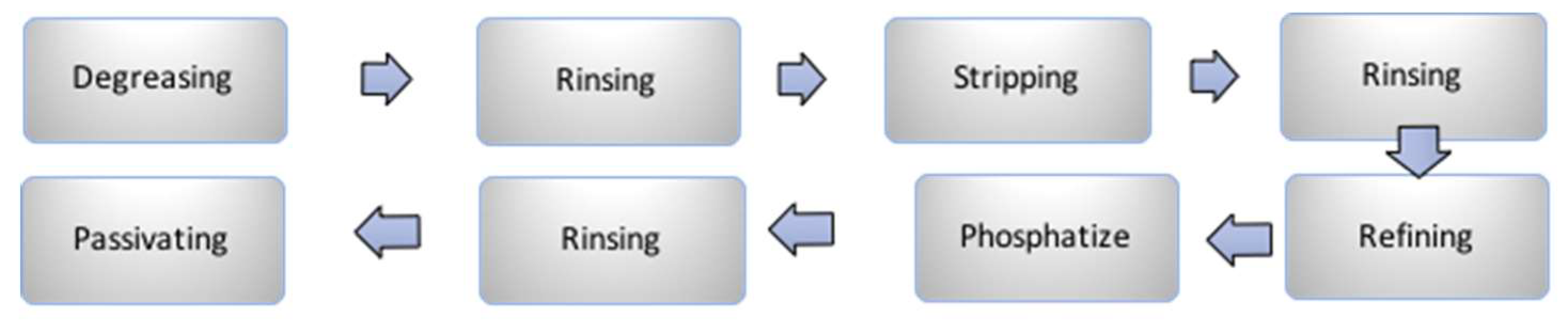
4.1. The Wastewater Recuperation Process

As commented before, first, the wastewater recuperation process was mapped, the resouces used (expenses) were identified, categorized and quantified. After that, the unitary cost of the reclaimed water was calculated. The necessary resources for wastewater treatment are:

• Liquid Aluminum Sulfate
• Liquid Caustic Soda
• Anionic Polymer
• Hydrated lime.

Table 1. Data from the wastewater treatment station.

Materials	Total Expenses ($)	Driver	Qtty	Unitary Cost ($)
Liquid Caustic Soda	$621.76	kg	460.56	$1.35
Liquid Aluminum Sulfate	$1534.50	kg	1395.00	$1.10
Hydrated lime	$56.50	kg	113.00	$0.50
Anionic Polymer	$958.32	kg	726.00	$1.32
ENERGY Pump 1	$116.00	kW	232.00	$0.50
ENERGY Pump 2	$3.08	kW	6.15	$0.50
ENERGY Pump 3	$40.00	kW	80.00	$0.50
ENERGY Pump 4	$60.00	kW	120.00	$0.50
ENERGY Extractor	$116.00	kW	232.00	$0.50
ENERGY Extractor	$176.00	kW	352.00	$0.50
Operator	$500.00	$500.00
Specialist	$400.00	$2000.00	$400.00
Slugde	$625.00	kg/d × 20 d	12,500	0.05
TOTAL Expenses Wastewater treatment plant ($)			$5207.15

shows the expenses incurred by the wastewater treatment station, their drivers, the consumed quantities and the calculated unitary cost per driver. It is worth noting that those activities are performed or controlled by a single operator.

Subsequently, the cost of the treated water was calculated using the volume produced in a month.

Table 2. Wastewater station’s Production volume.

Product	Unit	Quantity		Unitary Cost
Treated Water	M3/day × 20 days	800 m3		$6.51/ m3
Sludge	kg/day × 20 days	12,500 kg	$0.05/kg	$625.00

shows this information.

Note that in the last column of Table 2 the costs of the recovered water ($/m³) and the monthly amount of sludge generated in kg/month are presented. This sludge, as already mentioned, is sent for an external deposit, with a cost of $0.05/kg. That cost is allocated to the treated water. After that, that cost was used as a resource cost in the surface treatment process. As it will be noted later, some selected activities and object costs consume such a resource.

4.2. Costs Computation

To calculate the cost of the cost objects (considering the surface treatment line) and according to the fuzzy activity-based costing methodology, all the activities related to that process were mapped. In the production process, specifically in the manufacturing and painting sectors, there is a dust painting chamber. All the metallic parts and components that go through this painting process (seat frames and window frames) need to have previously gone to the surface treatment baths sector. The sequence of steps of the surface treatment process is shown in the flowchart of Figure 8.

The first stage of cost appropriation corresponds to the allocation of the resource costs to the mapped activities. As such, all the expenses, including the cost of the recovered water, incurred by the company during the period under analysis were listed.

Table 3. Resources and drivers in surface treatment plant.

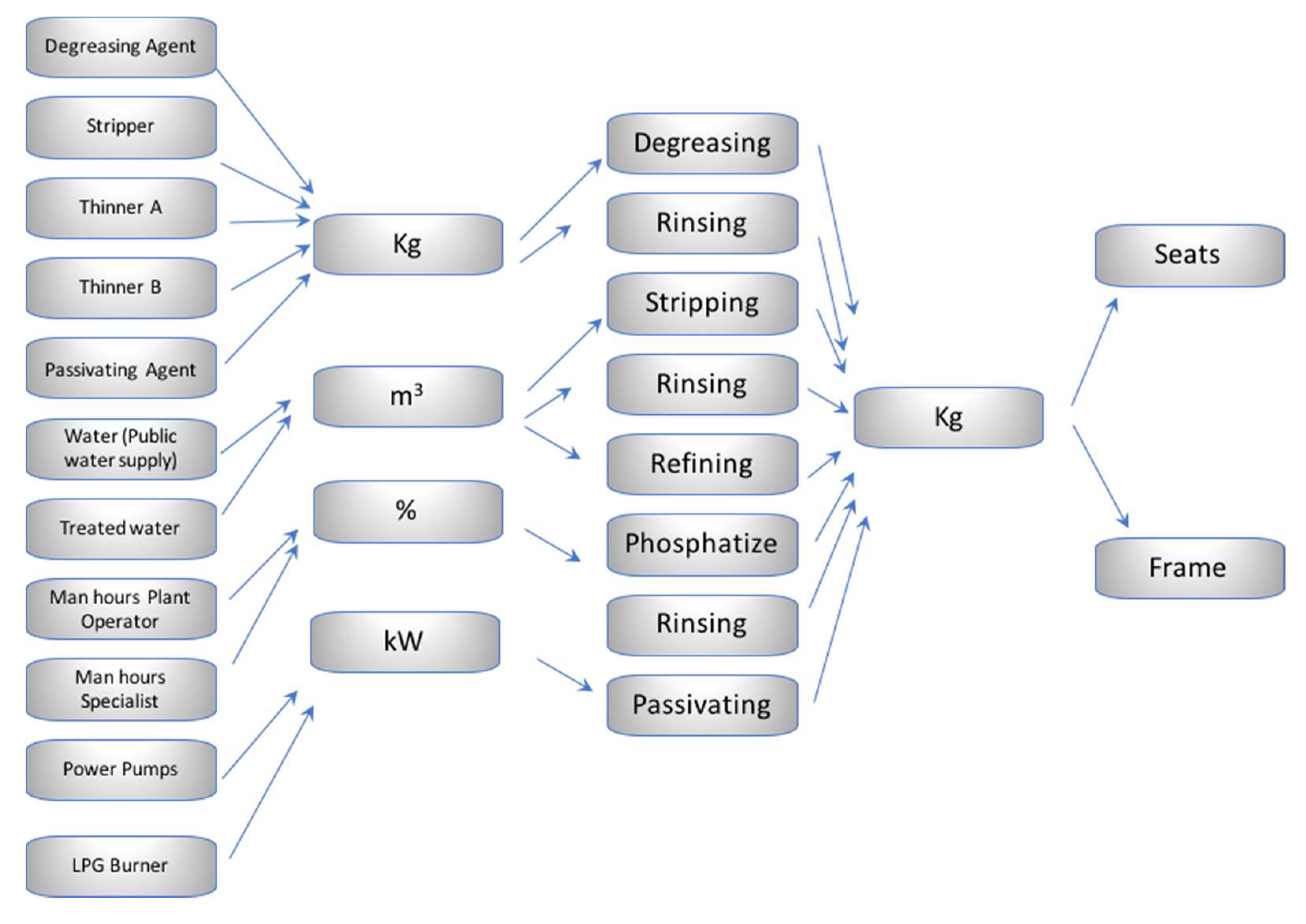
Resources	Driver
Degreasing Agent	kg
Stripper	kg
Thinner A	kg
Thinner B	kg
Passivating Agent	kg
Water (Public water supply)	M3
Recycled water	M3
Manhours (Plant Operator)	$
Manhours (Specialist)	$
Power Pump 1	kW
Power Pump 2	kW
LPG Burner 1	M3/d
LPG Burner 2	M3/d

shows those resources and their correspondent drivers.

Figure 5 shows the resources drivers used to allocate the activity costs to the activities. In the case of the engineering specialist and the operator, the direct labour costs (total remuneration) were prorated based on the time spent by these persons in these activities. This information was obtained from the timesheet that the organization itself manages for these purposes. In the same Figure 9, the drivers used to allocate the activity costs into the products are also shown.

After a qualitative observation, it was concluded that such values presented an important variation during the period under analysis; this was caused mainly because this production plant produces its vehicles on demand and the lot sizes vary considerably. This fact induces a great variation in product characteristics and into the production levels of some parts and systems. To tackle this difficulty and uncertainty in determining the expenses and production volumes and, in order to obtain better costs measures and enhance the long-term decision-making process, it was decided to introduce the fuzzy numbers approach. The fuzzy (i.e., triangular) numbers were defined using the lower and the higher costs observed during an operating year. Therefore, all the expenses in the surface treatment plant were transformed into triangular numbers. After that, such expenses were represented using its matrix representation ($\tilde{r}$_j) and the triangular numbers are shown below:

$${\tilde{r}}_j=\left[\begin{array}{c}\left(213,313,413\right)\\ \left(544,665,768\right)\\ \left(458,502,656\right)\\ \left(456,672,789\right)\\ \left(4356,5173,6782\right)\\ \left(126,190,301\right)\\ \left(876,937,1022\right)\\ \left(345,400,457\right)\\ \left(342,456,671\right)\\ \left(23,44,59\right)\\ \left(34,44,54\right)\\ \left(2011,2415,2980\right)\\ \left(2300,2415,2500\right)\end{array}\right]$$

Note, in this survey the cost of the treated water was considered as a resource of the process (r7) consumed by the surface treatment activities. Following, the resource-activity matrix was constructed. For that, an interview with the plant managers was carried out. After that, the quantities of each resource driver during the last year were mapped, and the limit values were translated into a fuzzy matrix representation. The resulting resource activity matrix is shown below ($\tilde{r}$_ij):

$${\tilde{r}}_{ij}=\left[\begin{array}{ccccccccccccc}\left(100,120,130\right)& 0& 0& 0& 0& \left(1,2,4\right)& 0& \left(17,33,45\right)& \left(1,2,3\right)& \left(22,23,26\right)& 0& \left(2195,2234,2400\right)& 0\\ 0& 0& 0& 0& 0& 0& \left(43,50,53\right)& \left(23,24,25\right)& \left(1,2,3\right)& \left(22,24,26\right)& 0& 0& 0\\ 0& \left(700,720,750\right)& 0& 0& 0& \left(1,2,3\right)& 0& \left(14,15,16\right)& \left(1,2,3\right)& \left(33,26,27\right)& 0& \left(2200,2356,2450\right)& 0\\ 0& 0& 0& 0& 0& -& \left(43,50,78\right)& \left(34,38,39\right)& \left(1,2,3\right)& \left(22,23,24\right)& 0& 0& 0\\ 0& 0& \left(150,155,176\right)& 0& 0& \left(48,54,56\right)& 0& \left(14,17,23\right)& \left(1,2,3\right)& 0& \left(22,23,26\right)& 0& \left(1880,2189,2234\right)\\ 0& 0& 0& \left(700,731,750\right)& 0& -& \left(23,25,28\right)& \left(17,18,22\right)& \left(1,2,3\right)& 0& \left(24,23,26\right)& 0& \left(2345,2450,2567\right)\\ 0& 0& 0& 0& 0& -& \left(23,35,38\right)& \left(2,4,5\right)& \left(1,2,3\right)& 0& \left(22,25,27\right)& 0& 0\\ 0& 0& 0& 0& \left(50,55,58\right)& \left(48,57,57\right)& 0& \left(34,35,42\right)& \left(1,2,3\right)& 0& \left(22,23,24\right)& 0& 0\end{array}\right].$$

Following, the calculations of the costs of the activities (${\tilde{a}}_i$) using triangular numbers were carried out:

$${\tilde{a}}_i=\left[\begin{array}{c}\left(\$1312.85,\$1641.82,\$2062.43\right)\\ \left(\$360.33,\$405.60,\$469.55\right)\\ \left(\$1644.80,\$1996.40,\$2423.89\right)\\ \left(\$446.10,\$499.36,\$573.19\right)\\ \left(\$1670.41,\$1820.49,\$2102.00\right)\\ \left(\$1912.14,\$2221.68,\$2432.74\right)\\ \left(\$89.91,\$110.06,\$143.73\right)\\ \left(\$4647.46,\$5530.60,\$7244.46\right)\end{array}\right]$$

The second stage of the method consists in allocating the costs of the activities to the products (cost objects). For this purpose, it was necessary to identify the activity drivers. After a simple observation process, it was defined that the only driver chosen for allocating the costs of the activities is the number of kilograms of the product that goes through each one of the activities of the surface treatment process. In Figure 10, it can be seen that there are activities that only serve one type of product, the seats, in such a way that the entire cost of those activities will be allocated to the product “seat frames”.

The a_ki matrix shows how, in percentages, the products consume the identified activities (driver).

$$a_{ki}=\left[\begin{array}{cccccccc}90\%& 90\%& 90\%& 90\%& 100\%& 100\%& 100\%& 100\%\\ 10\%& 10\%& 10\%& 10\%& 0& 0& 0\%& 0\%\end{array}\right]$$

Consequently, it is enough to divide the cost of the activity by the total of kilograms processed by each activity to obtain the unit cost of the driver, to multiply that unit cost by the total of kilograms of each product and to obtain the unit cost of the treatment surface for each product produced. Finally, it was possible to calculate the product cost in the surface treatment section. This is done by multiplying its respective weight by the sum of the unit costs of the activities.

The matrix ${\tilde{p}}_k$ shows the total costs (fuzzy representation) allocated to the two products classes, seat frames and windows frames, respectively:

$${\tilde{p}}_k=\left[\begin{array}{c}(\$11,719.74,\$13,786.34,\$16,916.93)\\ (\$364.26,\$439.66,\$535.07)\end{array}\right]$$

Such a matrix shows the total costs (using triangular representation) of each of the products. After that, to obtain the correspondent unitary cost of each one of the products, those amounts had to be divided by the total quantity in kilograms that were treated within the surface treatment tanks. For this objective, two triangular numbers were defined using the limits of the production levels (in kilograms) for each class of products $({\widetilde{PL}}_k$).

$${\widetilde{PL}}_k=\left[\begin{array}{c}(140000,141680,150000)\\ (15000,28020,30000)\end{array}\right]$$

Finally, the values of the ${\widetilde{PL}}_k$ were divided by ${\tilde{p}}_k$ to obtain the values of the unitary costs associated to the surface treatment costs using the triangular representation.

Table 4. Final calculation of the unitary costs of the surface treatment plant.

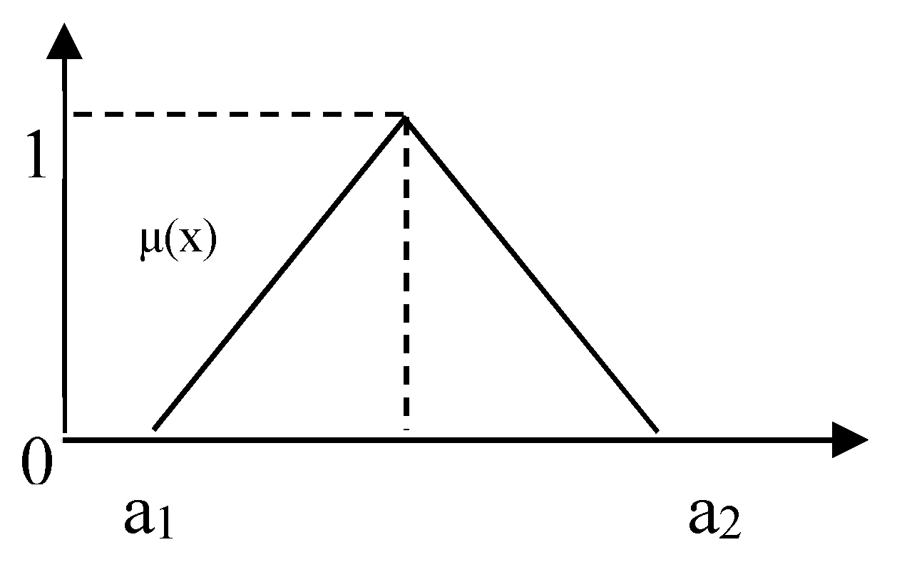
	Unitary Costs (Triangular) $/u	Unitary Cost (Crisp) $/u
Seat Frames	(0.08, 0.10, 0.11)	$0.10
Window Frames	(0.02, 0.02, 0.02)	$0.02

shows the unitary costs of each product type using the triangular representation and their respective crisp values.

5. Conclusions

The need and importance of implementing economic studies on wastewater treatment costs and its impact is evident. The present work is about the development and application of a fuzzy-based activity-based costing method to calculate the production costs in a surface treatment plant, which uses as an input treated wastewater produced by the same plant. Additionally, since in many cases there are substantial levels of variability and uncertainty in data, the proposed method includes a fuzzy representation of the main parameters of the method. To do that, triangular numbers were used to incorporate that aspect and to increase the realism of the obtained values. The use of activity-based costing allows the correct allocation of the costs related to the effluents treatment and the use of triangular numbers allows dealing with uncertainty in a better way.

Since the cost of the treated water is reverted into the process that actually generates these wastes, the proposed methodology can help to measure how expensive it is to generate waste and the impact it has on the recovery process represented here by the wastewater treatment process.

Additionally, this method allows managers to perform controls and implement useful indicators which provide better quantitative information on the performance and behaviour of important drivers, improving decision making efficiency.

References

- Burritt, R.; Schaltegger, S. Accounting towards sustainability in production and supply chains. Br. Account. Rev. 2014, 46, 327–343. [Google Scholar] [CrossRef]
- Noodezh, H.R.; Moghimi, S. Environmental costs and environmental information disclosure in the accounting systems. Int. J. Acad. Res. Account. Finance Manag. Sci. 2015, 5, 13–18. [Google Scholar] [CrossRef]
- Jabbour, C.J.C.; de Sousa Jabbour, A.B.L.; Govindan, K.; Teixeira, A.A.; de Souza Freitas, W.R. Environmental management and operational performance in automotive companies in Brazil: The role of human resource management and lean manufacturing. J. Clean. Product. 2013, 47, 129–140. [Google Scholar] [CrossRef]
- Yang, M.G.M.; Hong, P.; Modi, S.B. Impact of lean manufacturing and environmental management on business performance: An empirical study of manufacturing firms. Int. J. Product. Econ. 2011, 129, 251–261. [Google Scholar] [CrossRef]
- Okafor, G.O.; Okaro, S.C.; Egbunike, F.C. Environmental cost accounting and cost allocation (A study of selected manufacturing companies in Nigeria). Eur. J. Bus. Manag. 2013, 5, 68–75. [Google Scholar]
- Kim, J.; Jeong, S. Economic and Environmental Cost Analysis of Incineration and Recovery Alternatives for Flammable Industrial Waste: The Case of South Korea. Sustainability 2017, 9, 1638. [Google Scholar]
- Cagno, E.; Micheli, G.J.; Trucco, P. Eco-efficiency for sustainable manufacturing: An extended environmental costing method. Product. Plan. Control 2012, 23, 134–144. [Google Scholar] [CrossRef]
- Nicolăescu, E.; Alpopi, C.; Zaharia, C. Measuring corporate sustainability performance. Sustainability 2015, 7, 851–865. [Google Scholar] [CrossRef]
- Senthil, K.D.; Ong, S.K.; Nee, A.Y.C.; Tan, R.B. A proposed tool to integrate environmental and economical assessments of products. Environ. Impact Assess. Rev. 2003, 23, 51–72. [Google Scholar] [CrossRef]
- Campos, L.M.D.S.; Trierweiller, A.C.; Carvalho, D.N.D.; Santos, T.H.S.D.; Peixe, B.C.S.; Bornia, A.C. Selection process theoretical framework on environmental costs: An exploratory vision. Latin Am. J. Manag. Sust. Dev. 2015, 2, 47–63. [Google Scholar] [CrossRef]
- Molinos-Senante, M.; Mocholí-Arce, M.; Sala-Garrido, R. Estimating the environmental and resource costs of leakage in water distribution systems: A shadow price approach. Sci. Total Environ. 2016, 568, 180–188. [Google Scholar] [CrossRef] [PubMed]
- Henri, J.F.; Boiral, O.; Roy, M.J. Strategic cost management and performance: The case of environmental costs. Br. Account. Rev. 2016, 48, 269–282. [Google Scholar] [CrossRef]
- Szadziewska, A. Corporate environmental costs–classification and disclosures in external reports. Zesz. Teoretyczne Rachunkowości 2012, 65, 45–70. [Google Scholar]
- Ruiz-Rosa, I.; García-Rodríguez, F.J.; Mendoza-Jiménez, J. Development and application of a cost management model for wastewater treatment and reuse processes. J. Clean. Product. 2016, 113, 299–310. [Google Scholar] [CrossRef]
- Sgroi, M.; Vagliasindi, F.G.; Roccaro, P. Feasibility, sustainability and circular economy concepts in water reuse. Curr. Opin. Environ. Sci. Health 2018, 2, 20–25. [Google Scholar] [CrossRef]
- Insel, G.; Gumuslu, E.; Cokgor, E.U.; Olmez-Hanci, T.; Tas, D.O.; Babuna, F.G.; Dizge, N. The Effect of Wastewater Reuse on Product Quality for an Oven Manufacturing Plant. In Proceedings of the Sixth International Conference on Environmental Management, Engineering, Planning & Economics, Thessaloniki, Greece, 25–30 June 2017. [Google Scholar]
- Insel, G.; Gumuslu, E.; Yuksek, G.; Ucar, S.N.; Cokor, U.E.; Hanci, O.T.; Erturan, O. Evaluation of water reuse in a metal finishing industry. In Proceedings of the 18th International Symposium on Environmental Pollution and its Impact on Life in the Mediterranean Region, Crete, Greece, 26–30 September 2015; pp. 27–30. [Google Scholar]
- Sato, T.; Qadir, M.; Yamamoto, S.; Endo, T.; Zahoor, A. Global, regional, and country level need for data on wastewater generation, treatment, and use. Agric. Water Manag. 2013, 130, 1–13. [Google Scholar] [CrossRef]
- Water, U.N. Managing Water under Uncertainty and Risk, the United Nations World Water Development Report 4; UN Water Reports; World Water Assessment Programme: Paris, France, 2012. [Google Scholar]
- The United Nations World Water Development Report, WWDR. Water for a Sustainable World 2015; UNESCO: Paris, France; Available online: http://unesdoc.unesco.org/images/0023/002318/231823E.pdf (accessed on 21 May 2018).
- Hetzer, K. Cash Flows Where Water Does. UNEP FI 2007, 7, 4–6. [Google Scholar]
- Vergine, P.; Salerno, C.; Libutti, A.; Beneduce, L.; Gatta, G.; Berardi, G.; Pollice, A. Closing the water cycle in the agro-industrial sector by reusing treated wastewater for irrigation. J. Clean. Product. 2017, 164, 587–596. [Google Scholar] [CrossRef]
- Costantino, F.; Di Gravio, G.; Tronci, M. Integrating environmental assessment of failure modes in maintenance planning of production systems. Appl. Mech. Mater. 2013, 295, 651–660. [Google Scholar] [CrossRef]
- Güven, D.; Hanhan, O.; Aksoy, E.C.; Insel, G.; Çokgör, E. Impact of paint shop decanter effluents on biological treatability of automotive industry wastewater. J. Hazard. Mater. 2017, 330, 61–67. [Google Scholar] [CrossRef] [PubMed]
- Piao, W.; Kim, Y.; Kim, H.; Kim, M.; Kim, C. Life cycle assessment and economic efficiency analysis of integrated management of wastewater treatment plants. J. Clean. Product. 2016, 113, 325–337. [Google Scholar] [CrossRef]
- Faraji, T.; Maghari, A.; Mirsepasi, N. A framework for assessing cost management system changes: The case of activity-based costing implementation at food industry. Manag. Sci. Lett. 2015, 5, 413–418. [Google Scholar] [CrossRef]
- Tsai, W.H.; Lin, T.W.; Chou, W.C. Integrating activity-based costing and environmental cost accounting systems: A case study. Int. J. Bus. Syst. Res. 2010, 4, 186–208. [Google Scholar] [CrossRef]
- Abdulbaki, D.; Al-Hindi, M.; Yassine, A.; Najm, M.A. An optimization model for the allocation of water resources. J. Clean. Product. 2017, 164, 994–1006. [Google Scholar] [CrossRef]
- Yuksek, G.; Okutman Tas, D.; Ubay Cokgor, E.; Insel, G.; Kirci, B.; Erturan, O. Effect of eco-friendly production technologies on wastewater characterization and treatment plant performance. Desalinat. Water Treat. 2016, 57, 27924–27933. [Google Scholar] [CrossRef]
- Kreuze, J.G.; Newell, G.E. ABC and life-cycle costing for environmental expenditures. Strat. Financ. 1994, 75, 38. [Google Scholar]
- Lockhart, J.; Taylor, A. Environmental considerations in product mix decisions using ABC and TOC. Manag. Account. Quart. 2007, 9, 13. [Google Scholar]
- Rodríguez Rivero, E.J.; Emblemsvåg, J. Activity-based life-cycle costing in long-range planning. Rev. Account. Financ. 2007, 6, 370–390. [Google Scholar] [CrossRef]
- Sun, Y.; Carmichael, D.G. Uncertainties related to financial variables within infrastructure life cycle costing: A literature review. Struct. Infrastruct. Eng. 2017. [Google Scholar] [CrossRef]
- Farr, J.V.; Faber, I.J.; Ganguly, A.; Martin, W.A.; Larson, S.L. Simulation-based costing for early phase life cycle cost analysis: Example application to an environmental remediation project. Eng. Econ. 2016, 61, 207–222. [Google Scholar] [CrossRef]
- Woodward, D.G. Life cycle costing—Theory, information acquisition and application. Int. J. Proj. Manag. 1997, 15, 335–344. [Google Scholar] [CrossRef]
- Zadeh, L.A. Information and control. Fuzzy Sets 1965, 8, 338–353. [Google Scholar]
- Nachtmann, H.; Needy, K.L. Methods for handling uncertainty in activity-based costing systems. Eng. Econ. 2003, 48, 259–282. [Google Scholar] [CrossRef]
- Yang, C.H.; Lee, K.C.; Chen, H.C. Incorporating carbon footprint with activity-based costing constraints into sustainable public transport infrastructure project decisions. J. Clean. Prod. 2016, 133, 1154–1166. [Google Scholar] [CrossRef]
- Goh, Y.M.; Newnes, L.B.; Mileham, A.R.; McMahon, C.A.; Saravi, M.E. Uncertainty in Through-Life Costing—Review and Perspectives. IEEE Trans. Eng. Manag. 2010, 57, 689–701. [Google Scholar] [CrossRef]
- Afonso, P.S.; Paisana, A.M. An Algorithm for Activity-Based Costing Based on Matrix Multiplication. In Proceedings of the 2009 IEEE International Conference on Industrial Engineering and Engineering Management, Hong Kong, China, 8–11 December 2009. [Google Scholar]
- Byrne, P. Fuzzy DCF: A Contradiction in Terms, or a Way to Better Investment Appraisal. 1997. Available online: http://citeseerx.ist.psu.edu/viewdoc/summary?doi=10.1.1.98.6802 (accessed on 4 June 2018).
- Díaz-Madroñero, M.; Satorre, J.R.; Mula, J.; López-Jiménez, P.A. Analysis of a wastewater treatment plant using fuzzy goal programming as a management tool: A case study. J. Clean. Prod. 2018, 180, 20–33. [Google Scholar] [CrossRef]
- Gregory, J.R.; Montalbo, T.M.; Kirchain, R.E. Analyzing uncertainty in a comparative life cycle assessment of hand drying systems. Int. J. Life Cycle Assess. 2013, 18, 1605–1617. [Google Scholar] [CrossRef]
- Kishk, M. Combining various facets of uncertainty in whole-life cost modelling. Const. Manag. Econ. 2004, 22, 429–435. [Google Scholar] [CrossRef]
- Kishk, M.; Al-Hajj, A. A fuzzy model and algorithm to handle subjectivity in life-cycle costing-based decision-making. J. Financ. Manag. Prop. Constr. 2002, 5, 93–104. [Google Scholar]
- Chiu, C.Y.; Park, C.S. Fuzzy cash flow analysis using present worth criterion. Eng. Econ. 1994, 39, 113–138. [Google Scholar] [CrossRef]
- Chang, D.Y. Applications of the extent analysis method on fuzzy AHP. Eur. J. Operat. Res. 1996, 95, 649–655. [Google Scholar] [CrossRef]