Article

Dynamic Panel Data Estimation in Accounting Research: System GMM as a Benchmark for Financial Statement Analysis


by
Maria Kalogera
*,
Antonios Georgopoulos
,
Eleftherios Aggelopoulos
and
Ioannis Ch. Lampropoulos
Department of Business Administration, University of Patras, 26504 Patras, Greece
*
Author to whom correspondence should be addressed.
Account. Audit. 2026, 2(3), 16; https://doi.org/10.3390/accountaudit2030016
Submission received: 29 June 2026 / Revised: 21 August 2026 / Accepted: 25 August 2026 / Published: 1 September 2026

Abstract

Dynamic panel data methods, and System GMM in particular, have become a methodological reference point in accounting research, yet their diagnostic performance has rarely been validated against the structural conditions characteristic of Southeast European (SEE) panels, namely SME dominance, short time horizons, and crisis-period volatility. This article applies and evaluates the System GMM estimator as a methodological benchmark for analysing dynamic accounting performance in Southeast European (SEE) panels. Firm-level performance indicators, most notably profitability and productivity, alongside export outcomes, exhibit precisely the econometric characteristics the Blundell–Bond estimator is designed to address persistence, bidirectional causality, and unobserved heterogeneity. Treated as performance-measurement constructs for management control and decision support, these measures are analysed in a firm-level panel of 284 Greek companies (ICAP DataPrisma, 2005–2017). Hansen and AR(2) diagnostics are not rejected across all specifications, establishing a reproducible methodological benchmark for accounting research under SEE conditions. The study further documents the estimator’s alignment with the standards of leading accounting journals, positioning it as an appropriate benchmark for analysing the dynamic evolution of accounting variables under the conditions examined.

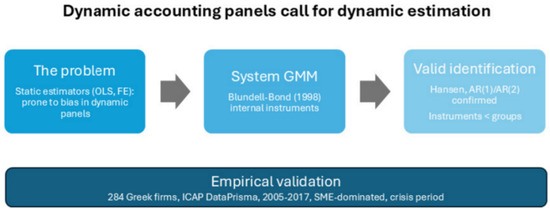
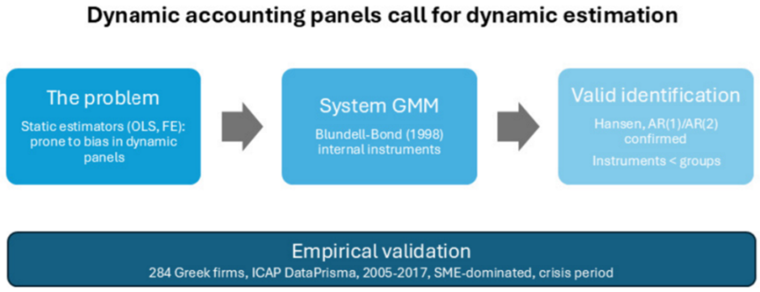
Graphical Abstract

1. Introduction

A balance sheet records the cumulative consequences of past decisions rather than a snapshot taken in isolation. Financial ratios carry their history with them: a firm’s return on equity in year t is shaped by its value in year t − 1, because the assets, financing structure, and retained earnings that produce it persist over time. This persistence is a property of how accounting information is generated, not an artefact of measurement. When an empirical model ignores it, the estimates it produces can misrepresent the relationships the study set out to measure.
Static estimators such as OLS and fixed effects are poorly suited to this setting. Applied to accounting panels, they tend to return biased and inconsistent results, for two reasons that are structural rather than incidental: unobserved differences between firms, and the dependence of each variable on its own past. Ref. [1] showed that the second of these alone biases the fixed-effects estimator in short panels, and the difficulty compounds when both are present. The choice of estimator therefore determines whether the reported relationships can be trusted.
Dynamic panel estimators were developed to address this combination of persistence and unobserved heterogeneity. The approach of [2], extended by [3] into the System GMM estimator, was built for panels with many cross-sectional units observed over short time spans, the structure that most firm-level accounting data share. Its adoption in journals such as Management Accounting Research, The Accounting Review, and European Accounting Review reflects a settled methodological position: claims about causality in accounting data are difficult to sustain without dynamic estimation.
The practical guidance on how to specify System GMM well, set out in [4,5], was developed largely with reference to large, stable corporate panels from advanced Western economies. Southeast European accounting panels depart from that setting in ways that matter for estimation. They are dominated by small and medium-sized firms, cover short time spans of roughly ten to thirteen years, run through periods of severe crisis-driven volatility, and sit within thinner institutional environments. Each of these features places additional strain on instrument validity, finite-sample behaviour, and the stability of the moment conditions the estimator relies on. Whether the standard guidance carries over to such data cannot be assumed; it has to be tested, and so far few studies have done so systematically. The present study takes up that task, using a short, unbalanced, SME-dominated panel of Greek companies that spans the crisis years to examine how the estimator’s diagnostics behave under conditions typical of the region.
On this basis, this study argues that System GMM is the appropriate estimator for accounting panels in the Southeast European context. Section 2 examines the features of financial statement data that create the estimation problem, and Section 3 sets out how System GMM resolves it. Section 4 applies the estimator to the ICAP panel, treating profitability and productivity as performance-measurement constructs for management control and decision support, and Section 5 reports the diagnostic tests that establish the validity of the results. Section 6 situates the findings within the international methodological literature, and Section 7 presents key conclusions. Throughout, the Greek firm-level panel is the empirical ground for the argument: it embodies the structural conditions of SME dominance, short horizons, and crisis volatility under which accounting researchers in the region typically work, and it shows that System GMM supports identification under them.

2. The Structural Econometric Problems of Accounting Data

Establishing why System GMM is the appropriate estimator first requires a precise account of the econometric problems that financial statement panels present. Four such problems recur in accounting research, and each one defeats simpler estimation strategies in a distinct way. Together they define the requirements that any adequate empirical design must meet.

2.1. Dynamic Persistence: Accounting Inertia

Financial statement variables are strongly autocorrelated over time, and that persistence has structural roots rather than incidental ones. Established customer relationships, accumulated specialised human capital, and brand equity all carry forward from one period to the next, and together with a firm’s accounting policy choices they hold reported figures on a stable path. Accounting numbers do not jump from year to year; they evolve as the business does. The standard way to capture this dependence is to place a lagged dependent variable, Yi, t − 1, on the right-hand side of the regression.
Doing so inside a fixed-effects model, however, creates a problem of its own. Ref. [1] showed that the lagged dependent variable introduces a bias of order O(1/T) that does not disappear as the cross-section grows. This bias is especially damaging in accounting research, where panels of financial statements are typically short, with T of roughly 5 to 15 years. It renders OLS and fixed effects estimates inconsistent and unsuitable for dynamic accounting analysis, which is what motivates the move to System GMM. The structure of modern financial data, in which the number of firms far exceeds the number of periods (N > T), reinforces the choice: under these conditions, GMM delivers consistent estimates [4,5] while accommodating the non-strict exogeneity that is built into accounting data, where current performance follows from earlier strategic decisions. Including the lagged dependent variable also encodes a substantive economic assumption, that firm behaviour evolves gradually rather than in abrupt steps [6].

2.2. Endogeneity and Bidirectional Causation

Clean, one-directional causality is rare in accounting research. More often the relevant forces operate in both directions at once, which complicates any attempt to read the data correctly. The link between export performance and profitability is a clear example. More profitable firms can absorb the high fixed costs of entering foreign markets and often build the necessary know-how before they begin to export. Once abroad, exposure to global competition and new sources of information feeds back into productivity, a mechanism usually called export learning. Firms that face capital constraints, by contrast, may never reach that point, because limited liquidity forecloses cross-border expansion.
When the relationship runs both ways, the explanatory variables end up correlated with the error term, which is the textbook form of endogeneity that pervades accounting research. Ordinary least squares are no longer adequate here, since its estimates are biased. The usual remedy is to find instruments, but in practice this is very hard: variables that are both exogenous and genuinely relevant are difficult to isolate among the tightly interlinked items of a set of financial statements. Ref. [2] addressed this by formalising a GMM approach that builds on the earlier instrumental-variable strategy of [7], whose authors first proposed first-differencing to remove fixed effects and using lagged levels as instruments, though without exploiting the full set of moment conditions that GMM uses. Rather than searching for external instruments that may not exist, the method draws on the lagged values of the variables themselves, which is its central advantage and the most dependable way to recover how the variables actually move over time.

2.3. Unobserved Heterogeneity of Firms: Accounting Policies and Management Quality

A further difficulty is the presence of unobserved, time-invariant firm characteristics that are correlated with both the explanatory and the dependent variables. In financial reporting, these include the aggressiveness of a firm’s accounting policies, expressed through the timing of revenue recognition or the choice of depreciation method, as well as the quality of its governance and the character of its organisational culture. None of these appears directly on the balance sheet, yet each shapes the numbers that do. Fixed-effects estimators try to eliminate this heterogeneity through the within-group transformation, but at a real cost: they discard all time-invariant information and, when a lagged dependent variable is present, reintroduce the Nickell bias, leaving the estimates inconsistent.
The Difference GMM estimator [2] removes the heterogeneity by taking first differences, but it weakens sharply when the variables are highly persistent, because the first-differenced instruments become weak. System GMM [3] resolves this by estimating the equations in levels and in differences together, which restores strong identification even when persistence is extreme. This combination, handling unobserved heterogeneity while retaining the information contained in the levels of the variables, is what makes System GMM a particularly suitable choice for empirical work on the dynamic, multidimensional nature of accounting data.

2.4. Measurement Error in Accounting Variables

Financial statement data also carry measurement errors, because accounting standards leave considerable discretion in how items are recognised and measured. That discretion serves the informational needs of management, but it introduces noise into the regressors and produces attenuation bias under OLS: coefficients are pulled artificially towards zero, so researchers systematically understate the true relationships between financial variables. System GMM addresses this through the strategic use of multiple lags as instruments for the affected variables. Averaging across lags dampens the measurement error specific to any single period and restores the accuracy of the estimates, so that the results reflect the underlying economic relationships rather than the imperfections of the reporting process.

3. System GMM Architecture and Accounting Justification

Having set out the structural econometric problems of accounting data, the analysis now turns to the mechanism through which System GMM addresses each of them, and to why the alternative estimators fall short of what a valid analysis of financial statement panels requires. The strength of System GMM is not its technical sophistication as such, but its capacity to accommodate the dynamic nature of accounting information, which the static estimators cannot.

3.1. The Blundell–Bond System GMM Estimator

The dynamic panel data model used by the System GMM for estimating financial performance relationships takes the following general form:
Yi,t = ci + β1 Yi,t−1 + β2 Xi,t + β3 Zi,t + Year Dummiest + εi,t
Here Yi,t is the performance measure for firm i in year t. The lagged term Yi,t−1 captures the dynamic persistence and time dependence that characterise accounting data. The vector Xi,t collects the main explanatory variables, which are treated as potentially endogenous because they frequently stand in a bidirectional relationship with the dependent variable. The vector Zi,t collects control variables taken as strictly exogenous, describing structural features of the firm, while the year dummies absorb common external shocks. Unobserved heterogeneity enters through ci, which holds the time-invariant characteristics of firm i, such as organisational culture. The final term, εi,t, is the idiosyncratic error, assumed to be independent and identically distributed. Specified this way, the model lets the System GMM estimator address endogeneity and the Nickell bias at the same time.
The estimator [3] combines two sets of moment conditions. The first is the Arellano–Bond set from the first-differenced equation, in which lagged levels serve as instruments. The second, which matters most for the present analysis, comes from the level equation and uses lagged first differences as instruments. Bringing the two together improves efficiency and reduces the finite-sample bias of the simpler Difference GMM estimator. The gain is substantial in accounting research, where financial variables are highly persistent: in that setting the lagged-level instruments used by Difference GMM become weak, and System GMM preserves identification where the alternatives tend to fail.

3.2. Internal Instruments: Accounting Justification

Using lagged values of the endogenous variables as instruments carries an accounting interpretation that standard econometric treatments usually leave implicit. Lagged accounting values meet the two conditions an instrument must satisfy, relevance and exogeneity. They are relevant because past performance predicts current performance through the accounting inertia described in Section 2. They are reasonably exogenous because, once the fixed firm effect is removed, past values cannot be driven by unexpected shocks to current profitability. The internal instrument structure of GMM is therefore well matched to the temporal structure of financial data.
This matters because external instruments that satisfy the exclusion restriction are, for most financial variables, almost impossible to find. It is very hard, for instance, to name a variable that influences a firm’s export activity without also bearing directly on its profitability, and such clean instruments are rare in practice. System GMM sidesteps the problem by drawing identification from the time structure of the panel itself, which is a more dependable basis than the questionable external instruments that appear in parts of the applied literature.

3.3. Why Not OLS, Fixed Effects or Random Effects?

Table 1 provides a systematic comparison of estimators for dynamic accounting panels, evaluating how System GMM addresses the four structural problems highlighted in Section 2.
Read from top to bottom, the table traces a progression. Pooled OLS fails on every count: it ignores firm-level heterogeneity entirely and, by treating endogenous regressors as exogenous, returns estimates that are biased and inconsistent. Fixed effects remove the time-invariant heterogeneity, but at the price of the Nickell bias once a lagged dependent variable enters the model, which is precisely the setting of dynamic accounting data. Random effects are more efficient in principle, yet they rest on the assumption that the firm effects are uncorrelated with the regressors, which rarely holds when accounting policy and management quality drive both. Instrumental-variable and two-stage least-squares estimators can address endogeneity, but only with external instruments that satisfy the exclusion restriction, and for most financial variables such instruments are not available.
The two GMM estimators resolve these problems internally. Difference GMM removes heterogeneity through first differencing and instruments the endogenous variables with their own past values, but it loses identifying power when the series are highly persistent, as accounting variables typically are, because the lagged-level instruments become weak. System GMM closes this gap by estimating the level and first-differenced equations jointly, which restores strong identification under persistence while retaining the information contained in the levels. System GMM allows researchers to account for all four econometric features simultaneously, making it an appropriate empirical choice for evaluating dynamic financial statement relationships under the conditions analysed in this study.

4. Processing and Empirical Analysis

The empirical analysis applies the System GMM estimator to a firm-level panel of Greek companies (ICAP DataPrisma), where profitability and productivity serve as performance measurement constructs for management control and decision support. A successful application at the firm level shows that the estimator supports identification in panel financial statement data of the kind that characterises the region.

4.1. Sample Structure and Variables

The analysis draws on a panel of Greek firms compiled from the ICAP DataPrisma database for the period 2005–2017. ICAP drew a stratified random sample of 284 manufacturing firms spanning 24 sectors of the Greek economy, subject to two inclusion criteria: an equal split of exporting and non-exporting firms (142 each) and data availability for at least 9 of the 13 annual periods per variable. Every firm is recorded across all thirteen years (3692 firm-year records); item-level missing values in certain performance variables and the loss of initial periods to lagging reduce the effective estimation samples to 2384–2669 observations across the reported specifications. The data form a structurally complete panel covering thirteen years, spanning the shift from pre-crisis expansion to the deep recession of 2010–2017. Because the number of firms far exceeds the number of years (N > T), the panel is well suited to System GMM, and the crisis period introduces substantial temporal variation that is useful for studying how firms adjust.
The sample comprises 284 firms, split evenly between 142 exporters and 142 non-exporters to keep the two groups comparable. Small and medium-sized enterprises dominate, accounting for 221 of the firms, which mirrors the actual structure of Greek business. It spans both traditional sectors (154 firms in food, textiles, wood, and paper) and higher-technology sectors (130 firms in chemicals, pharmaceuticals, IT, and mechanical equipment). Export status is a time-invariant, firm-level classification: a firm is designated an exporter if its export-to-sales ratio is at least 50% in each of its observed years. Any imbalance in the estimation samples concerns the performance variables, which have item-level missing values, not the export classification, which is fixed for each firm. The sample is split by design into equal numbers of exporting and non-exporting firms, since export activity is the focus of the study. As a time-invariant regressor, export status is absorbed by the within transformation under fixed effects and is identified only through the level equation of the system GMM estimator. Prior to estimation, the data were screened for outliers. Extreme values, identified through boxplot inspection, were treated by winsorizing the affected performance variables, including ROE, at the 5th and 95th percentiles. This bounds the influence of extreme observations, including firms with near-zero or negative equity that would otherwise inflate equity-scaled ratios, without discarding observations, and explains the bounded ranges reported in the descriptive statistics.
Table 2 lists the variables and their roles in the model.
Before the dynamic estimates, the following Table 3 and Table 4 summarise the data. The performance ratios are bounded (for example, ROE ranges from −0.28 to 0.38 and EBITDA/equity from −0.10 to 0.75), so the estimates are not driven by extreme values or by firms with negative equity, and the covariates are only weakly correlated.

4.2. Financial Performance: Productivity and Profitability (RQ1–RQ4)

The analysis addresses four research questions on the dynamic determinants of firm performance, measured through profitability and productivity, and on how export orientation, firm size, and the macroeconomic environment shape it.
RQ1. 
How is export activity associated with overall economic performance, measured through productivity and profitability?
RQ2. 
How does firm size (SME status) shape the relationship between export intensity and overall performance?
RQ3. 
How does the onset of the financial crisis alter the dynamic relationship between export orientation and firm performance?
RQ4. 
What is the joint effect of firm size and the crisis on the relationship between export activity and performance?
Table 5 reports four parallel one-step System GMM models. The dependent variables are labour productivity (LP), return on equity (ROE), and two EBITDA-based measures of operating profitability, scaled (a) by equity and (b) by total assets. Because EBITDA strips out depreciation, interest, and taxes, these two measures capture the firm’s underlying cash-generating capacity and can be read as indicators of operating resilience, that is, the capacity to sustain performance through adverse conditions, which is especially pertinent over a sample period dominated by the crisis. Estimating the same relationships across these alternative definitions also tests the stability of the findings, confirming that they do not hinge on a single measure of financial performance.
Estimation is by one-step System GMM [3] in Stata13 using xtabond2, with forward orthogonal deviations [8] and heteroskedasticity-robust standard errors with a finite-sample correction. The regressors fall into three groups by their identifying assumptions. First, the lagged dependent variable and capital structure are treated as endogenous and instrumented GMM-style with their own lagged levels of order two and higher. Second, firm size and the size–export interactions are time-invariant at the firm level and are therefore treated as strictly exogenous; because a time-invariant regressor is by construction uncorrelated with the idiosyncratic shocks, its contemporaneous values are valid instruments, and it is identified through the levels equation rather than the first-differenced equation, in which time-invariant regressors are eliminated. Third, firm age, the crisis dummy, and the sector, location, and year dummies are treated as exogenous controls; liquidity is treated as an exogenous instrument in the ROE and EBITDA models. Export status is likewise time-invariant by construction, since firms are classified as exporters or non-exporters for their entire observed period, which is what makes the fixed 142/142 split well defined; it too is identified through the levels equation, and its lagged values coincide with its level, so the estimates are unaffected by its instrumental treatment. Identification of the time-invariant terms through the levels equation rests on the standard system-GMM assumption that they are orthogonal to the firm-specific unobserved effects; this is supported here by the sampling design, in which export status and firm size are fixed by construction rather than outcomes of within-sample performance, and by the inclusion of sector and location controls, which absorb major sources of firm-level heterogeneity.
For the endogenous regressors, lag depth was set by role and by the persistence of the series. For the persistent dependent variables (ROE and EBITDA/equity) and the capital-structure regressor, GMM-style instruments use lags from the second up to the thirteenth (L2–L13); for the less persistent dependent variables (labour productivity and EBITDA/total assets), shallower lags suffice (L2–L3). These ranges were not fixed a priori but set, per model, to the shortest depth yielding valid diagnostics without instrument proliferation. The instrument matrix is collapsed [5] throughout, so instrument counts remain well below the number of groups (88–100 for 281–282 groups). That this design avoids over-instrumentation is confirmed by the Hansen statistics (p = 0.10–0.18), which lie in a healthy range rather than near one; the difference-in-Hansen tests (p = 0.51–0.94) assess the additional level moment conditions that distinguish the system estimator and are likewise not rejected. This parsimony guards against instrument proliferation and preserves the power of the Hansen test, the central reporting requirement for any dynamic panel study.
Across all four models, the lagged dependent variable is highly significant (p < 0.01), with coefficients ranging from 0.503 (ROE) to 0.819 (LP), which confirms that firms’ financial figures carry a strong memory of their past. Methodologically, this is what System GMM is designed to accommodate: a static model could not capture this dynamic and would return seriously biased estimates.
The Arellano–Bond test confirms first-order (p < 0.001) but no second-order serial correlation (p = 0.200). The Hansen J test does not reject the overidentifying restrictions (p = 0.102), and the difference-in-Hansen test does not reject the exogeneity of the additional level instruments (p = 0.813), supporting the use of system rather than difference GMM.
Export activity, the main explanatory variable, is negatively correlated with all of the profitability measures on its own. Its real contribution emerges only through the interaction terms, which reveal the conditions under which exporting becomes advantageous. For the second research question (RQ2), the Export Activity × SME term is positive in every model but is interpreted through the joint interaction tests and combined marginal effects reported below rather than through the individual coefficient. On that basis the size–export interaction is supported for labour productivity, where the interaction terms are jointly significant and the combined marginal effect is positive, while for the profitability measures the interaction terms are not jointly significant, so a corresponding profitability advantage cannot be established from these data. This evidence thus provides statistical support for a productivity advantage among exporting SMEs, while remaining inconclusive for profitability.
The crisis (RQ3) reveals a telling asymmetry. Export firms managed to raise their productivity (0.194, p < 0.05), most likely through intensified survival efforts, but this gain did not carry over into higher profitability, which marks the limit of the ‘export shield’ against so deep and prolonged a recession.
The triple interaction (SME × Export Activity × Crisis) exposes a weak point in the resilience of smaller firms: despite their overall advantage, exporting SMEs could not sustain their productivity edge at the height of the crisis, held back by fragile supply chains and limited access to finance that left them more exposed to shocks.
To assess the interaction structure formally, the joint significance of all interaction terms is tested in each model. In the labour-productivity model they are jointly significant (Wald F(4281) = 2.71, p = 0.030); combining the relevant coefficients, the total marginal effect of export status for SMEs during the crisis is positive and significant (0.340, p = 0.012), indicating that exporting SMEs sustained higher productivity through the crisis. For the profitability measures, the interaction terms are jointly insignificant (ROE, p = 0.105; EBITDA/equity, p = 0.134; EBITDA/assets, p = 0.055), so the crisis is interpreted as reshaping productivity dynamics rather than profitability. Correlations among the main covariates are low (the highest is 0.34, between capital structure and liquidity), so multicollinearity is not a concern for the core regressors; any imprecision in the higher-order interaction terms reflects the limited number of large exporting firms rather than collinearity among the main variables.
Finally, the control variables fit the broader picture. Size (SME status) is generally associated with lower returns than for large firms, consistent with economies of scale, while liquidity carries a negative sign, suggesting that accumulated cash can at times mask inefficient use of capital structure. The diagnostic statistics, reported in Section 5, indicate that the models are statistically sound and that the moment conditions are not rejected by the data.

5. Diagnostic Checks: Validation of the GMM Specification

All models are estimated with the one-step System GMM estimator. Two-step GMM with [9] finite-sample correction is asymptotically more efficient, but the one-step estimator is adopted here as the baseline: in finite samples the two-step standard errors can be downward-biased even after the Windmeijer correction, which makes one-step the more conservative and reliable basis for inference [4,9,10], in simulations calibrated to panels of comparable dimensions, find that the one-step estimator minimises bias and yields more dependable standard errors, which reinforces this choice. System GMM is also preferred over its Difference counterpart for the reason it suits persistent accounting data: under the firm-level heterogeneity and high persistence of this sample, the system estimator is the more robust of the two [11]. One-step results are reported throughout for consistency and comparability across all specifications.

5.1. The Hansen Test

The [12] J test evaluates the null hypothesis that the instruments are jointly valid and uncorrelated with the error term. A low p-value rejects validity, but a value approaching unity is itself a warning sign of instrument proliferation. Following [5], sound practice keeps the p-value within roughly 0.10 to 0.25, which balances validity against statistical power, particularly when the sample is limited. In every model here the Hansen p-value fell within this range, confirming that lagged accounting values act as legitimate instruments for the endogenous financial variables.

5.2. The Arellano–Bond AR(2) Test

The Arellano–Bond test for second-order serial correlation in the first-differenced residuals, AR(2), is the decisive check on the core GMM assumption that the error term is not serially correlated in levels. First-order correlation, AR(1), is expected and is a normal feature of models estimated in first differences, but second-order correlation would invalidate the second-lag instruments. In every model, the AR(2) p-value lay well above conventional thresholds, so the null of no second-order autocorrelation cannot be rejected, which confirms the validity of the moment conditions.

5.3. Instrument Count Discipline

Too many instruments can produce a spuriously clean Hansen test [12], masking weaknesses in the specification. The risk is acute in panel data, where combining multiple lags with several time periods quickly inflates the number of moment conditions. To guard against it, the instrument count was held strictly below the number of firms in every specification, the same purpose served by the collapse option noted above. This keeps the diagnostic tests at full power and the estimates reliable, in line with the standards expected in contemporary accounting research, as summarised in the compliance checklist of Table 6.
Beyond these instrument-based diagnostics, the specification was also checked for stability across the alternative performance measures reported in Section 4—labour productivity, return on equity, and the two EBITDA-based measures. The estimated relationships hold across all of them, confirming that the findings do not depend on a single definition of financial performance, as recorded in the final row of Table 6.

5.4. Comparison with Static Estimators and Robustness Across GMM Variants

To show with this study’s own data that static estimators are biased for these dynamic relationships and that the findings do not depend on a single GMM variant, the same specification was estimated by five estimators: pooled OLS, fixed effects, one-step System GMM, two-step System GMM with Windmeijer-corrected standard errors, and Difference GMM. Table 7 reports, for all four models, the coefficient on the lagged dependent variable, the size–export interaction, the joint test of all interaction terms, and the GMM diagnostics.
Three patterns emerge. First, the coefficient on the lagged dependent variable is bracketed in every model by the upward-biased pooled OLS estimate and the downward-biased fixed-effects estimate, with the System GMM estimate falling between these bounds—the pattern predicted by [1,4]. Pooled OLS overstates persistence by conflating it with unobserved firm heterogeneity, whereas fixed effects understate it through the downward Nickell bias in short panels. The System GMM estimates are stable across the one- and two-step forms. Second, the joint significance of the size–export interaction for labour productivity is confirmed under both one- and two-step System GMM (p = 0.030 and p = 0.004), while the profitability interactions remain jointly insignificant throughout; the substantive conclusion—a productivity advantage for exporting SMEs, with profitability inconclusive—is therefore not an artefact of the one-step estimator. Third, under Difference GMM, the level information on the time-invariant regressors is discarded: the main export and firm-size terms drop out of the first-differenced equation, and the size–export interaction, identified only through its overlap with the time-varying crisis structure, is estimated imprecisely and is not jointly significant. This weak identification of near-time-invariant terms under Difference GMM is precisely the limitation that the system estimator was designed to overcome [3], and the difference-in-Hansen tests do not reject the additional level moment conditions on which System GMM relies. Taken together, these results provide direct empirical support, on the authors’ own data, for adopting System GMM as the benchmark estimator.
It should be noted that while the Hansen and AR(2) diagnostic tests confirm that the specified moment conditions are not rejected by the data, they do not automatically prove causal validity or theoretical priority. Instead, they serve as crucial specification checks demonstrating that the System GMM estimator is empirically well-behaved and appropriate under the specific conditions of the analysed sample.

6. What GMM Identification Changes: Evidence from Literature

The methodological case made in Section 2 and Section 3 is not only theoretical. A body of empirical work across accounting and corporate finance has shown, in concrete and replicable terms, what GMM identification changes relative to static estimators, and what would have been concluded incorrectly had OLS or Fixed Effects been used instead. These studies share a consistent pattern: static estimators distort the magnitude, direction, or causal interpretation of relationships between financial variables, and GMM corrects those distortions in ways that change the substantive conclusions.
Ref. [13] offers perhaps the clearest case in the capital structure literature. Estimating a large panel of US firms with System GMM, the authors found that firms move toward their target leverage ratios far faster than OLS or Fixed Effects imply, a result that overturns a substantial body of prior work and reshapes how financial flexibility is understood. The distortion came from exactly the Nickell bias that affects Fixed Effects models with a lagged dependent variable, the bias documented in Section 2.1. Ref. [14] shows something similar for the link between export activity and firm liquidity: estimated dynamically rather than statically, it reveals a link from exporting to stronger financial health that OLS obscures behind simultaneity bias. Ref. [15] reaches an analogous conclusion for working capital and SME profitability, where GMM uncovers a negative relationship between the cash conversion cycle and profitability that cross-sectional OLS had overstated because of unobserved firm heterogeneity. Across these cases, the lesson is the same: the choice of estimator is not a technical formality but the difference between reliable and unreliable conclusions. The findings of the present study should be read in this light, since the performance relationships identified in the ICAP panel can be interpreted more reliably because the estimation strategy corrects for the biases that would otherwise undermine them.
The Growing Use of GMM in Leading Journals
Table 8 summarises the studies discussed above together with further applications across the breadth of accounting and finance research. Following the adoption of GMM from the foundational work of [2,3] through to recent corporate finance applications shows that handling endogeneity and temporal dependence properly can materially affect the reliability of conclusions drawn from panel financial data.
As the review makes clear, System GMM is now applied across the whole range of financial reporting: from earnings quality [16] and capital structure [12] to export performance and profitability [15]. Refs. [14,17] are of particular relevance here, since both documents that export activity and its relationship to firm performance are inherently dynamic and cannot be identified reliably by static estimators. The present study carries this line of validation into the Southeast European context, showing that the same specification discipline, controlling for accounting inertia, correcting for bidirectional causality, and holding the instrument count in check, supports identification in an SME-dominated Greek firm panel. That evidence, under the specific conditions of Southeast European accounting data, is this study’s primary contribution to methodological literature.
Table 8. Representative studies adopting dynamic GMM methods in accounting and finance research.
StudyMagazineGMM ApplicationAccounting Variable
[2]Rev. Econ. StudiesDifference GMMEmployment, investments
[3]J. EconometricsSystem GMMProduction functions
[12]J. Corporate FinanceSystem GMM—capital structureIndicators leverage (Balance sheet)
[14]J. Int. EconomicsDynamic GMMexport market participation decision/export status/export intensity (robustness checks), liquidity
[15]J. Business Finance & Acc.System GMMWorking capital, profitability
[18]J. Financial EconomicsDynamic (system) GMMBoard structure, firm performance (ROA, Tobin’s Q)

7. Theoretical Rationale and Concluding Remarks

The empirical validation in this study centres on the ICAP firm-level panel, where System GMM delivered consistent identification under the conditions that characterise Southeast European accounting research: short panels, SME dominance, and crisis-period volatility. The result is a reproducible methodological benchmark for accounting research carried out under these conditions.
This preference follows from the nature of accounting variables rather than from any taste for technical sophistication. An accounting figure is determined by carrying financial information forward through time, which makes temporal continuity part of its structure. Every number on a balance sheet is an accumulated result of flows that began in earlier years and end in the present. Whether a study concerns earnings quality or capital structure, the same logic holds that accounting measures have a memory that must be modelled rather than set aside. Static methods have their place in genuinely cross-sectional work, but using them on dynamic accounting data calls for a strong justification that is, in most cases, simply absent.
Seen this way, a static regression that treats each observation as a separate, independent event is a poor representation of the accounting process. System GMM addresses this by building time dependence directly into the model, so that the lagged variable is no longer a statistical nuisance to be removed but a structural feature of the underlying economic reality. It is this correspondence between the method and the object it studies that distinguishes substantive analysis from estimation without theoretical grounding.
Drawing on the firm-level evidence from the ICAP panel and on the comparison with applications published in leading journals, this study has shown that System GMM can handle endogeneity, unobserved heterogeneity, and the dynamic persistence of accounting variables at the same time. For researchers working with panel financial statements, particularly in the SME-dominated, short-panel settings typical of the Southeast European region, System GMM is a methodologically appropriate benchmark, provided it is applied with the specification discipline and diagnostic validation set out here.

Author Contributions

Conceptualization, M.K., A.G., E.A. and I.C.L.; methodology, M.K., E.A.; writing-original draft preparation, M.K.; writing-review and editing, M.K., E.A. and I.C.L.; supervision, A.G. All authors have read and agreed to the published version of the manuscript.

Funding

This research received no external funding.

Institutional Review Board Statement

Not applicable.

Informed Consent Statement

Not applicable.

Data Availability Statement

Restrictions apply to the availability of these data. Data were obtained from the ICAP DataPrisma database and are available from the authors with the permission of the ICAP DataPrisma database.

Conflicts of Interest

The authors declare no conflicts of interest.

Abbreviations

The following abbreviations are used in this manuscript:
2SLSTwo-Stage Least Squares
ABArellano–Bond (estimator)
AR(2)Second-order autocorrelation (Arellano–Bond test)
BBBlundell–Bond (estimator)
DVDependent Variable
EBITDAEarnings Before Interest, Taxes, Depreciation, and Amortization
GLSGeneralized Least Squares
GMMGeneralized Method of Moments
ICAPICAP DataPrisma firm-level database (data source)
IVInstrumental Variables
LPLabor Productivity
NNumber of cross-sectional units (firms)
OLSOrdinary Least Squares
ROAReturn on Assets
ROEReturn on Equity
RQResearch Question
SEESoutheast Europe
SMESmall and Medium-sized Enterprise
TNumber of time periods

References

  1. Nickell, S. Biases in dynamic models with fixed effects. Econometrica 1981, 49, 1417–1426. [Google Scholar] [CrossRef] [Scilit]
  2. Arellano, M.; Bond, S. Some tests of specification for panel data: Monte Carlo evidence and an application to employment equations. Rev. Econ. Stud. 1991, 58, 277–297. [Google Scholar] [CrossRef] [Scilit]
  3. Blundell, R.; Bond, S. Initial conditions and moment restrictions in dynamic panel data models. J. Econom. 1998, 87, 115–143. [Google Scholar] [CrossRef] [Scilit]
  4. Bond, S.R. Dynamic panel data models: A guide to micro data methods and practice. Port. Econ. J. 2002, 1, 141–162. [Google Scholar] [CrossRef] [Scilit]
  5. Roodman, D. How to do xtabond2: An introduction to difference and system GMM in Stata. Stata J. 2009, 9, 86–136. [Google Scholar] [CrossRef] [Scilit]
  6. Fiordelisi, F.; Molyneux, P. The determinants of shareholder value in European banking. J. Bank. Financ. 2010, 34, 1189–1200. [Google Scholar] [CrossRef] [Scilit]
  7. Anderson, T.W.; Hsiao, C. Formulation and estimation of dynamic models using panel data. J. Econom. 1982, 18, 47–82. [Google Scholar] [CrossRef] [Scilit]
  8. Arellano, M.; Bover, O. Another Look at the Instrumental Variable Estimation of Error-Component Models. J. Econom. 1995, 68, 29–52. [Google Scholar] [CrossRef] [Scilit]
  9. Windmeijer, F. A finite sample correction for the variance of linear efficient two-step GMM estimators. J. Econom. 2005, 126, 25–51. [Google Scholar] [CrossRef] [Scilit]
  10. Judson, R.A.; Owen, A.L. Estimating dynamic panel data models: A guide for macroeconomists. Econ. Lett. 1999, 65, 9–15. [Google Scholar] [CrossRef] [Scilit]
  11. Van Biesebroeck, J. Robustness of productivity estimates. J. Ind. Econ. 2007, 55, 529–569. [Google Scholar] [CrossRef] [Scilit]
  12. Hansen, L.P. Large sample properties of generalized method of moments estimators. Econometrica 1982, 50, 1029–1054. [Google Scholar] [CrossRef] [Scilit]
  13. Flannery, M.J.; Hankins, K.W. Estimating dynamic panel models in corporate finance. J. Corp. Financ. 2013, 19, 1–19. [Google Scholar] [CrossRef] [Scilit]
  14. Greenaway, D.; Guariglia, A.; Kneller, R. Financial factors and exporting decisions. J. Int. Econ. 2007, 73, 377–395. [Google Scholar] [CrossRef] [Scilit]
  15. García-Teruel, P.J.; Martínez-Solano, P. Effects of working capital management on SME profitability. Int. J. Manag. Financ. 2007, 3, 164–177. [Google Scholar] [CrossRef] [Scilit]
  16. Dechow, P.; Ge, W.; Schrand, C. Understanding earnings quality: A review of the proxies, their determinants and their consequences. J. Account. Econ. 2010, 50, 344–401. [Google Scholar] [CrossRef] [Scilit]
  17. Love, J.H.; Mansury, M.A. Exporting and productivity in business services: Evidence from the United States. Int. Bus. Rev. 2009, 18, 630–642. [Google Scholar] [CrossRef] [Scilit]
  18. Wintoki, M.B.; Linck, J.S.; Netter, J.M. Endogeneity and the dynamics of internal corporate governance. J. Financ. Econ. 2012, 105, 581–606. [Google Scholar] [CrossRef] [Scilit]
Table 1. Comparison of panel estimators’ data for dynamic accounting research.
EstimatorLagged DVEndogeneityUnobserved HeterogeneitySuitable for Persistent Dynamic Danels
OLS (Pooled)Biased and inconsistentNot addressedNot controlledUnsuitable
Fixed Effects (Within)Nickell biasTime-varying onlyRemoved by within transformationUnsuitable for dynamic panels
Random Effects (GLS)BiasedAssumes exogeneityPartially controlledOnly under restrictive assumptions
IV/2SLSRequires external instrumentsAddressed if instruments validDepends on specificationExternal instruments rarely available
Difference GMM (AB)Consistent (internal instruments)Internal instrumentsRemoved by first-differencingWeak instruments under high persistence
System GMM (BB)Consistent and efficientInternal instrumentsLevels-and-differences systemJointly addresses all four panel issues
Notes: DV = dependent variable, AB = Arellano–Bond, BB = Blundell–Bond.
Table 2. Variable definitions and operationalization (based on firm-level data extracted from ICAP DataPrisma, 2005–2017).
#Variable Role in the Model Definition
1ROEDependent variableNet Profit/Total Equity (%)
2EBITDA/EquityDependent variable (robustness)EBITDA/Equity
3EBITDA/Total AssetsDependent variable (robustness)EBITDA/Total Assets
4Labor ProductivityDependent variableSales/Total Employees (ln)
5Export ActivityMainly independent variable Binary: 1 = Exporter (export-to-sales ratio > = 50% in each observed year), 0 = Non-exporter
6SMEsModerator/Control (fixed at firm level)EU Recommendation 2003/361: 1 = SME, 0 = Large Enterprise
7CrisisModerator (macroeconomic framework)Binary: 1 = 2010–2017 (crisis), 0 = 2005–2009 (no expansion)
8Export Activity × SMEInteraction variable (size) Differentiated impact of export activity for SMEs versus large
9Export Activity × CrisisInteraction variable (crisis) Differentiated impact of export activity in a period of crisis
10SME × CrisisInteraction variable (size × crisis)Differentiated impact of the crisis for SMEs versus large firms
11SME × Export Activity × CrisisTriple interaction variable Combined effect of size and crisis on the export-performance relationship
12AgeControl variableYears from establishment to observation year (ln)
13Capital StructureControl variableEquity to Total Assets Ratio (ln)
14LiquidityControl variableCurrent Assets/Short-Term Liabilities (Current Ratio)
15SectorControl variableBinary: 1 = High technology, 0 = Traditional industry
16LocationControl variable Binary: 1 = Urban areas, 0 = Other areas
Table 3. Descriptive statistics.
VariableMeanSDMinMaxN
ROE0.0470.148−0.2820.3803639
Labor productivity11.9880.9524.65416.1563636
EBITDA/equity0.2170.207−0.0970.7483639
EBITDA/total assets0.0780.065−0.0340.2183639
SMEs (dummy)0.7500.433013692
Export Activity (dummy)0.5000.500013692
Crisis (dummy)0.6150.487013692
Firm Age3.2090.66305.0563688
Capital Structure−0.9690.734−7.511−0.0113537
Liquidity2.0772.2610.04649.6473639
Notes: N varies (3537–3692) owing to item-level missingness. ROE and productivity derive from a separate data file from the EBITDA measures.
Table 4. Correlation matrix.
ROELPEB/eqEB/taSMEsExpCrisisAgeCapital Struct.Liq
ROE1.00
Labor Productivity0.121.00
EBITDA/equity0.650.191.00
EBITDA/total assets0.660.150.651.00
SMEs (dummy)−0.03−0.07−0.00−0.041.00
Export Activity (dummy)−0.020.07−0.03−0.02−0.011.00
Crisis (dummy)−0.140.02−0.15−0.14−0.010.001.00
Firm Age−0.000.15−0.09−0.00−0.18−0.050.241.00
Capital Structure0.12−0.08−0.400.180.02−0.000.030.091.00
Liquidity−0.03−0.06−0.19−0.010.060.010.060.050.341.00
Notes: Pairwise correlations. Coefficients significant at p < 0.05 in the source output.
Table 5. One-step system GMM results.
Variable Labor ProductivityROEEBITDA/EquityEBITDA/Total Assets
L.lnproductivity0.8189 ***
(0.0554)
---
L.ROE-0.5025 ***
(0.0826)
--
L.EBITDA_Equity--0.6034 ***
(0.0553)
-
L.EBITDA_Total Assets---0.6433 ***
(0.0516)
Export Activity−0.0487
(0.1189)
−0.1724 ***
(0.0566)
−0.1264 **
(0.0564)
−0.0513 ***
(0.0169)
Export Activity × Crisis0.1939 **
(0.0755)
0.0398
(0.0306)
0.0376
(0.0299)
0.0130
(0.0081)
Export Activity × SME0.4112 ***
(0.1424)
0.1259 *
(0.0651)
0.1487 **
(0.0686)
0.0581 ***
(0.0217)
SME × Export Activity × Crisis−0.2158 **
(0.0941)
−0.0239
(0.0332)
−0.0273
(0.0356)
−0.0099
(0.0095)
SME × Crisis0.0666
(0.0556)
0.0255
(0.0306)
0.0211
(0.0292)
0.0066
(0.0079)
SMEs−0.2720 ***
(0.0902)
−0.1303 ***
(0.0495)
−0.1390 ***
(0.0466)
−0.0482 ***
(0.0158)
Age0.0226
(0.0254)
0.0060
(0.0094)
−0.0061
(0.00917)
−0.0004
(0.0031)
Capital Structure0.0883 ***
(0.0309)
0.0345 ***
(0.0012)
−0.0371 ***
(0.0143)
0.0081 **
(0.0035)
Liquidity−0.0132
(0.0124)
−0.0056 **
(0.0025)
−0.0047 *
(0.00262)
−0.0020 **
(0.0009)
Sector−0.0652 **
(0.0322)
0.0042
(0.0087)
−0.0028
(0.00851)
0.0021
(0.0029)
Location0.0070
(0.0457)
−0.0197 *
(0.0117)
−0.0045
(0.0156)
−0.0041
(0.0045)
Year DummiesYESYESYESYES
AR(1) p0.0000.0000.0000.000
AR(2) p0.1390.2000.5500.182
Hansen p0.1800.1020.1770.144
Diff-in-Hansen p0.5140.8130.6470.935
Observations 2407238426692669
Number of instruments < Number of Groups100 < 28296 < 28195 < 28288 < 282
Notes: Dependents variables: Labor Productivity, ROE, EBITDA/Equity, EBITDA/Total Assets. *** p < 0.01, ** p < 0.05, * p < 0.10. Standard errors in parentheses.
Table 6. Compliance with one-step System GMM validation rules across all model specifications.
One—Step System GMM Validation RuleResults Across All Reported Models
Lagged dependent variable statistically significant (1 year lag)
Hansen test
Control AR(2)
Number of Instruments < Number of Groups
Stability across alternative performance measures
Table 7. Robustness across estimators.
Pooled OLSFixed EffectsSystem GMM (1-Step)System GMM (2-Step)Difference GMM
Labour productivity
Lagged DV0.918 ***0.677 ***0.819 ***0.816 ***0.612 ***
Export × SME--0.411 ***0.376 ***0.318
Joint interaction test (p)--0.0300.0040.207
Hansen (p)--0.1800.1800.071
AR(2) (p)--0.1390.1330.127
Instruments--10010076
ROE
Lagged DV0.562 ***0.265 ***0.503 ***0.596 ***0.368 ***
Export × SME--0.126 *0.0630.027
Joint interaction test (p)--0.1050.3780.275
Hansen (p)--0.1020.1020.064
AR(2) (p)--0.2000.1230.316
Instruments--969665
EBITDA/equity
Lagged DV0.654 ***0.383 ***0.603 ***0.641 ***0.532 ***
Export × SME--0.149 **0.0910.067
Joint interaction test (p)--0.1340.2660.186
Hansen (p)--0.1770.1770.114
AR(2) (p)--0.5500.5000.678
Instruments--959565
EBITDA/total assets
Lagged DV0.723 ***0.392 ***0.643 ***0.630 ***0.477 ***
Export × SME--0.058 ***0.0340.099
Joint interaction test (p)--0.0550.3260.064
Hansen (p)--0.1440.1440.035
AR(2) (p)--0.1820.1670.275
Instruments--888865
Notes: Same specification across estimators. Robust standard errors; two-step System GMM uses Windmeijer-corrected standard errors. *** p < 0.01, ** p < 0.05, * p < 0.10. Under Difference GMM the main export and firm-size terms drop out of the first-differenced equation; the size–export interaction is identified only weakly, through its overlap with the time-varying crisis structure. The joint interaction test is a Wald test of all interaction terms.
Disclaimer/Publisher’s Note: The statements, opinions and data contained in all publications are solely those of the individual author(s) and contributor(s) and not of MDPI and/or the editor(s). MDPI and/or the editor(s) disclaim responsibility for any injury to people or property resulting from any ideas, methods, instructions or products referred to in the content.