Article

Evaluation of Water Vapor Feedback Using a Two-Layer Atmospheric Box Model


Department of Environmental Sciences, University of Yamanashi, 4-4-37, Takeda, Kofu 400-8510, Yamanashi, Japan
*
Author to whom correspondence should be addressed.
Mod. Math. Phys. 2026, 2(2), 4; https://doi.org/10.3390/mmphys2020004
Submission received: 8 January 2026 / Revised: 14 April 2026 / Accepted: 20 April 2026 / Published: 23 April 2026

Abstract

Massive-scale, ultra-high-resolution numerical simulations for climate change prediction provide data of exceptional accuracy and reliability. However, this comes at the cost of enormous computational resources, and the underlying processes often remain a “black box”. In contrast to these sophisticated methods, we theoretically analyzed the water vapor feedback effect using a highly simplified model that focuses exclusively on the most critical physical factors governing climate change. Specifically, we formulated a two-layer box model by dividing the entire atmosphere into layers of equal optical thickness. Using this model, we quantitatively verified the extent to which the water vapor feedback effect—a key driver of global warming—can be theoretically reproduced.

1. Introduction

The development of computer simulation models for predicting climate change, along with their associated computational techniques, has undergone significant advancement to date. The origins of the climate model trace back to the one-dimensional vertical model formulated by Manabe and Stricker in 1964 [1]. This model posits a columnar atmosphere extending vertically from the ground upward, describing the spatial distribution of atmospheric temperature with altitude under two conditions: radiative equilibrium and radiative-convective equilibrium. Using this model, it becomes possible to predict temperature changes resulting from a doubling of the atmospheric carbon dioxide level. This one-dimensional vertical model was later expanded into a three-dimensional general circulation model by Manabe and Bryan in 1969 [2]. The latter three-dimensional model consists of an atmospheric general circulation model, an oceanic general circulation model, and a two-dimensional heat/water balance model for continents, enabling the reproduction of both vertical and horizontal heat transport.
Climate models have continued to evolve and become increasingly complex [3,4]. Consequently, the state-of-the-art technology now enables the effective utilization of supercomputers equipped with approximately 5000 GPUs (graphics processing units) to run ultra-high-resolution climate simulation models [5]. Here, the term “resolution” refers to the degree to which the Earth’s surface is subdivided. For instance, a resolution value of 1 km means the Earth’s surface is divided into approximately 10 14 grid cells. Analyzing the exchange of energy and matter across all these regions requires an enormous computational cost. Indeed, the data volume handled by the CMIP6 (Coupled Model Intercomparison Project Phase 6), the international project underpinning the scientific basis of the IPCC’s Six Assessment Report, was estimated to range from approximately 20 to 40 petabytes [6]. As these facts illustrate, increasing computational accuracy and resolution inevitably lead to a massive increase in computational effort. Consequently, predicting climate change using these models requires substantial time and financial resources.
In the field of climate prediction, quantitative and highly accurate forecast data generated by large-scale computing is often required. Conversely, from an academic perspective, particularly in the field of physics, simplified theoretical models that extract the intrinsic essence of phenomena are often preferred [7,8]. By focusing solely on the critical physical factors governing climate change and omitting secondary ones, it becomes easier to establish governing laws and perform theoretical analysis of the phenomena. Furthermore, advancing analysis based on simplified models can transform complex concepts within the climate system into intuitive and comprehensible representations.
The present study adopts the latter approach, constructing a simplified radiative balance model that decomposes the entire atmosphere into two homogeneous layers. Using this model, we analyzed the water vapor feedback effect on atmospheric temperature and verified its quantitative validity. Water vapor is the primary contributor to the greenhouse effect on Earth, along with carbon dioxide (CO2) and methane [9]. An increase in atmospheric water vapor content accompanying rising temperatures is thought to produce a positive feedback effect, where the increased moisture further drives temperature rise [10]. We utilized an independently developed two-layer atmospheric box model to verify the extent to which this feedback effect, deeply involved in global warming, can be quantitatively reproduced.

2. Atmospheric Box Model

A box model is a simplified theoretical framework that discretizes a complex continuum into several discrete “boxes”. It accounts for the inflow, outflow, generation, and removal (sink) of physical quantities within and between these boxes. By dividing continuous space into multiple regions and assuming internal homogeneity, the model uses balance equations to describe the transport of matter and energy. This approach is widely applied not only in climate change analysis [11] but also in fields such as hydrology, carbon cycling, atmospheric and aquatic pollutant transport, and ecology [12,13,14,15].
In this study, we employ a two-layer box model that divides the atmosphere into two layers of equal optical thickness, accounting for radiative transfer between them. This model assumes a spatially uniform temperature within each layer and focuses exclusively on the interactions between four components: the Earth’s surface, the lower atmosphere, the upper atmosphere, and outer space. Compared to complex, large-scale climate models, this approach significantly reduces computational costs. By incorporating only the most critical physical factors into the radiation balance, the model enhances theoretical clarity and provides a better qualitative understanding of the phenomena, following the framework proposed by Goody and Walker (1972) [16]. The primary advantages of this model include its mathematical solubility with low computational effort, ease of tracking energy and material balances, and simplified sensitivity analysis. Its main limitation, however, is the inability to reproduce detailed spatial distributions due to the assumption of homogeneity within each box.
Notably, Manabe and Wetherald [17] demonstrated that temperature distributions calculated using 9-layer and 18-layer atmospheric models were nearly identical. This suggests that extending our two-layer model to three, four, or more layers may yield results that progressively converge toward the actual vertical temperature distribution.

3. Water Vapor Feedback

We analyze the feedback effects of water vapor using a two-layer atmospheric radiative balance box model. Water vapor is the most significant greenhouse gas on Earth, as it absorbs terrestrial radiation across a broader spectral range than other gases [18]. Therefore, fluctuations in water vapor content are expected to exert strong feedback on atmospheric temperature [19].
Here, “feedback” refers to natural mechanisms where initial climate alterations—such as changes in atmospheric or surface conditions—trigger subsequent changes that either amplify or suppress the original trend. For example, as global temperatures rise due to increased carbon dioxide concentrations, the atmospheric water vapor capacity increases. Since water vapor is a potent greenhouse gas, this increase further accelerates global warming, a process known as positive feedback. Conversely, rising global temperatures can promote surface water evaporation and ice melt, strengthening convection that transports heat from the surface upward. This enhanced upward heat flow can lead to a relative cooling of the surface, a process known as negative feedback. Beyond these examples, various feedback loops arising from changes in atmospheric water vapor content must be considered to understand their collective impact on the climate system.
The importance of examining water vapor feedbacks lies in the distinction between the climate’s initial trigger and its subsequent responses. While the primary driver of atmospheric changes—increased CO2 concentrations—is a direct consequence of anthropogenic activities, the ensuing mechanisms of temperature change are governed by the natural laws of physics. For example, the observed increase in atmospheric water vapor over the past two decades cannot be attributed to direct human emissions. Although activities such as irrigation and power plant cooling release water vapor, their contribution is negligible compared to the total observed increase [20]. This indicates that the rise in water vapor is primarily driven by natural feedback mechanisms. Nevertheless, the specific conditions under which these various feedbacks contribute to temperature change, as well as the relative strength and breakdown of their contributions, remain far from self-evident. Simplified climate models, such as the two-layer atmospheric box model, serve as powerful tools for theoretically elucidating these complex interactions. Motivated by this, the present study focuses on the following four physical factors, using a two-layer model to quantitatively estimate their feedback strengths and evaluate their respective influences on surface air temperature.
(1)
Enhancement of the Atmospheric Greenhouse Effect
This feedback stems from the direct amplification of the greenhouse effect. As previously discussed, rising temperatures increase atmospheric water vapor capacity. Since water vapor is a potent greenhouse gas, its accumulation further traps terrestrial radiation, leading to additional warming.
This mechanism constitutes a positive feedback for the following reasons: first, an enhanced greenhouse effect increases the absorption and re-emission of radiation by the atmosphere, raising surface temperatures (+). Second, this warming facilitates further increases in atmospheric water vapor, reinforcing the greenhouse effect (+). Since both steps amplify the initial warming, the net feedback is positive.
(2)
Increased Albedo Due to Cloud Cover
This feedback involves changes in the Earth’s reflectivity. An increase in water vapor often leads to greater cloud cover [21]. Low-level clouds, in particular, possess a high albedo and reflect a significant portion of incoming solar radiation back into space [22]. Consequently, increased cloudiness reduces the solar flux reaching the surface, exerting a cooling effect.
This is considered a negative feedback: rising surface temperatures increase cloud cover, which elevates the planetary albedo (+). However, this higher albedo reduces surface solar absorption, thereby lowering surface temperatures (−). Because the resulting temperature change opposes the initial warming, this feedback is negative.
(3)
Enhanced Latent Heat Transport
This factor focuses on the redistribution of energy through phase changes of water. Vast amounts of liquid water evaporate from the surface, absorbing energy and ascending as water vapor. As this vapor reaches the cooler upper atmosphere, it condenses into liquid (forming precipitation) and releases the stored energy. This process effectively pumps heat from the surface to the upper atmosphere.
Latent heat transport intensifies as temperatures rise because warmer air can carry more moisture, the primary medium for this transport. As this upward heat flux increases, it removes more energy from the surface, causing a relative cooling.
This constitutes a negative feedback: an initial rise in surface temperature boosts atmospheric water vapor and latent heat transport (+). The intensified transport then moves more heat away from the surface, leading to a temperature drop (−). The opposing directions of these effects result in a negative feedback.
(4)
Reduction of the Atmospheric Window Due to Increased Cloud Cover
The “atmospheric window” refers to the spectral band (approximately 8–12 µm) where the atmosphere is relatively transparent to outgoing terrestrial radiation. While most infrared radiation is absorbed by gases, radiation within this window typically escapes directly to space. However, increased cloud cover—particularly from high-level clouds—can “plug” this window by absorbing radiation that would otherwise escape [23].
As surface temperatures and water vapor levels rise, the resulting increase in cloud cover shrinks the atmospheric window, trapping more radiation within the Earth system.
This is a positive feedback: rising surface temperatures increase cloud cover, which reduces the amount of radiation escaping through the atmospheric window (−). A reduction in escaping radiation leads to higher surface temperatures (−). Since both components of the causal chain work to amplify the initial warming, this feedback is positive.

4. Two-Layer Radiative Equilibrium Model

4.1. Modeling Strategy

The four physical factors discussed in the previous section are all intrinsically linked to atmospheric water vapor content. Accordingly, our modeling strategy proceeds as follows. First, we formalize the dependence of atmospheric water vapor on surface temperature changes (Section 4.2). Next, we develop a radiative balance model to determine surface air temperature (Section 4.3 and Section 4.4). Surface temperature is governed by the energy balance of various radiative and absorptive processes, including incoming solar radiation, terrestrial emission into space, and the absorption and re-emission of radiation by atmospheric greenhouse gases. Since the four physical factors identified earlier also modulate this energy balance, we integrate them into a single governing equation for surface air temperature (Equation (19), presented later). By expressing surface temperature as a function of these four variables, we can quantitatively compare the individual feedback contributions of each factor to overall temperature changes (Section 5 and Section 6).

4.2. Dependence of Atmospheric Water Vapor Content on Earth’s Surface Temperature

This section formulates the total amount of water vapor contained in the atmosphere and explores how it depends on the Earth’s surface temperature. To simplify the discussion, the Earth is approximated as a perfect sphere, and the sphere’s radius R E is approximated as equal to the actual Earth’s equatorial radius (approximately 6.4 × 10 6 m). Strictly speaking, the Earth is an ellipsoid slightly bulging at the equator, but its flattening ratio is negligible at 3.35 × 10 3 , and thus can be ignored [24]. Minor spatiotemporal variations in sea level due to tides are also disregarded. Given the assumption, we consider a line segment connecting a point in space at height h above the Earth’s surface to the center of the Earth. Let S h and V h be the surface area and the volume, respectively, of the sphere with this line segment as its radius. Then the following equation holds:
S h = d V h d h = 4 π R E + h 2
By separating variables in this equation, the volume d V h of a spherical shell with thickness d h in the infinitesimal interval can be expressed as follows.
d V h = 4 π R E + h 2 d h
The amount of water vapor per unit volume (i.e., water vapor density) at a given altitude, denoted h , is denoted as ρ H 2 O h [mol/m3]. Integrating the product of ρ H 2 O h with d V h from the Earth’s surface h = 0 to the top of the troposphere h = h t r o p yields the total amount of water vapor contained within the troposphere, denoted by N H 2 O [mol] as
N H 2 O = ρ H 2 O h d V ( h ) = 4 π h = 0 h = h t r o p ρ H 2 O h R E + h 2 d h
On Earth, most water vapor is contained within the troposphere (the layer of air extending from the surface to approximately 11 km above), where vertical air movement (convection) is active. Therefore, this paper estimates the amount of water vapor in the atmosphere limited to the troposphere boundary layer (the upper edge of the troposphere). Note that while temperatures in the upper troposphere can drop below freezing, the presence of water vapor has been confirmed [25], so the entire troposphere, including its upper layers, is considered. Since the average height of the upper boundary of the troposphere is 11 km [26], we set h t r o p = 11,000 m.
Next, we determine the altitude ( h ) dependence of the water vapor density ρ H 2 O h contained in the integrand of Equation (3). The term e s T is employed to denote the vapor pressure at saturation, defined as the state at which the relative humidity (RH) is equivalent to 100%. The ideal gas law of state
P V = n R T
implies that N H 2 O can be expressed as
N H 2 O = e s T V R T
Here, R = 8.31 [J/(K·mol)] is the gas constant. Dividing both sides of Equation (5) by the volume V yields the molar density of water vapor, ρ H 2 O [mol/m3], as follows.
ρ H 2 O T = e s T R T
The temperature dependence of saturated vapor pressure e s ( T ) is expressed as follows using the Clausius–Clapeyron relation, which represents the slope of the vapor pressure curve [27].
e s T = e 0 · exp H H 2 O R H 2 O 1 T s 1 T h
Here, R H 2 O is the value obtained by dividing the gas constant R by the molar mass of water vapor (18 g/mol), resulting in 461.5 J/(K·kg) [26]. H H 2 O signifies the enthalpy of vaporization (heat of vaporization) of water, which is 2.45 × 10 6 J/kg at 1 atm and 25 °C [24]. It should be noted that while H H 2 O is a temperature-dependent quantity, its temperature dependence is negligible, with a decrease of only 2.53 × 10 3 J/kg per 1 °C increase. e 0 denotes the saturated vapor pressure at the Earth’s surface, with a value of 1689 Pa [24].
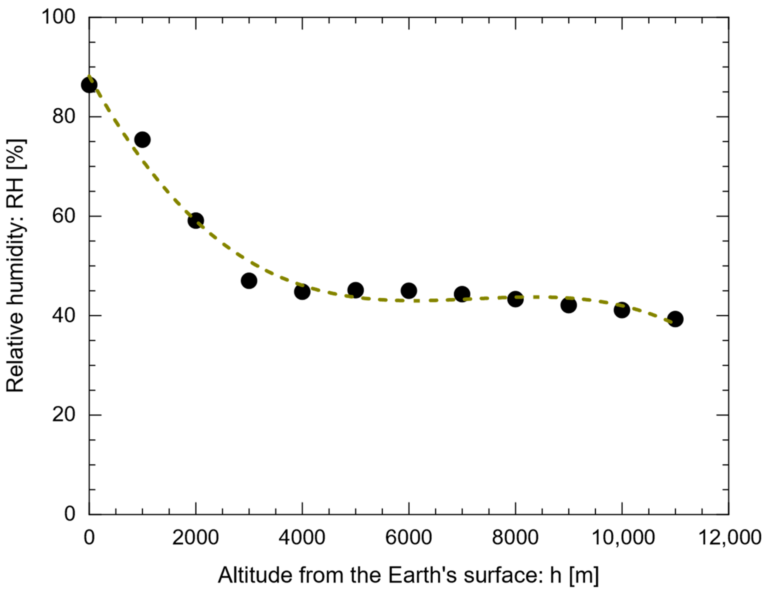
It is important to note that the discussion so far is valid only under the assumption that relative humidity (RH) is always RH = 100%. In the actual atmosphere, relative humidity decreases with increasing altitude. Figure 1 shows the altitude distribution of relative humidity and its approximation curve. The measured data shown in Figure 1 represents the average of monthly mean values for the vertical distribution of relative humidity, calculated using radiosonde observations from 353 locations worldwide over a 10-year period (1980–1989) [28]. The dotted line in Figure 1 represents the result of approximating this measured data with a third-order polynomial curve, expressed by the following polynomial R H h with respect to altitude h [m].
R H h = 1.28 × 10 12 h 3 + 2.78 × 10 8 h 2 1.96 × 10 4 h + 0.882
Similar to relative humidity R H h , the temperature T in the troposphere also declines with increasing altitude. Assuming a temperature lapse rate of Γ = 6.5 × 10 3 K/m and denoting the surface temperature as T s , the altitude dependence of temperature T is written by
T h = T s Γ h
Replacing e s T in Equation (6) with R H h e s T and converting the independent variable from T to h using Equation (9), the water vapor density at a given height h can be expressed as
ρ H 2 O h = R H h · e s h R · T h
Substituting Equation (10) into Equation (3) and performing the integration leaves only the surface air temperature T s as the sole variable on the right-hand side, as all others are constants.
N H 2 O T s = 4 π e 0 R h = 0 h = h t r o p R H h T s Γ h · exp H H 2 O R H 2 O 1 T s 1 T s Γ h R E + h 2 d h
Equation (11) establishes a correlation between the water vapor content, N H 2 O , and the surface air temperature, T s . This equation allows us to determine the increase in water vapor content N H 2 O when the surface air temperature T s changes.
It should be noted that the derivation above assumed that atmospheric temperature changes linearly with altitude (Equation (9)). However, the two-layer box model described later assumes that the temperature is uniform within each of the two stacked atmospheric layers. Therefore, in our actual calculations, we proceeded by discretizing the atmospheric temperature along altitude. See Appendix A for details.

4.3. Radiation Balance in the Two-Layer System

The Earth’s temperature is determined by the equilibrium between the solar radiation it receives and the terrestrial radiation it emits. These two fluxes are maintained in a constant state of balance. This is because nature possesses an inherent compensatory mechanism: even if a change in the atmosphere or the surface temporarily reduces the outgoing radiation, the system naturally adjusts to increase the radiation until energy balance is restored.
According to the Stefan-Boltzmann law, the energy E of electromagnetic waves emitted by a substance is proportional to the fourth power of its absolute temperature T assuming the substance acts as a blackbody—an idealized object that perfectly absorbs and emits incident electromagnetic radiation across all wavelengths. The Stefan-Boltzmann law reads as
E = σ T 4
Here, σ is the Stefan-Boltzmann constant, having a numerical value of 5.67 × 10 8 W·m−2·K−4. Therefore, even if the energy balance is temporarily disrupted, fluctuations in the temperature of the Earth’s surface and atmosphere cause changes in the radiant energy leaving the planet. Eventually, this radiant energy will balance the radiation coming from the Sun, leading to a new equilibrium. For example, even if increased atmospheric greenhouse effects cause more radiation to be reflected back to the surface, this raises surface temperatures, which in turn increases Earth’s outgoing radiation, leading to a new equilibrium. This process is called the Planck feedback and functions as a negative feedback mechanism inherent to Earth. Without it, Earth’s greenhouse effect is said to spiral out of control [29].
The mechanism of this radiation balance cannot be understood by considering only the radiation reaching Earth from the Sun and the radiation escaping from Earth into space. It is also necessary to account for solar radiation reflected by the Earth’s surface and clouds, as well as solar radiation and terrestrial radiation absorbed or re-emitted by the atmosphere. Furthermore, the heat exchange between the Earth’s surface and the atmosphere via convection and latent heat transport must also be considered. In this section, we construct a radiation balance model incorporating these factors and formalize the relationship between surface temperature and various energy transfers (the derived result is shown as Equation (19) later).
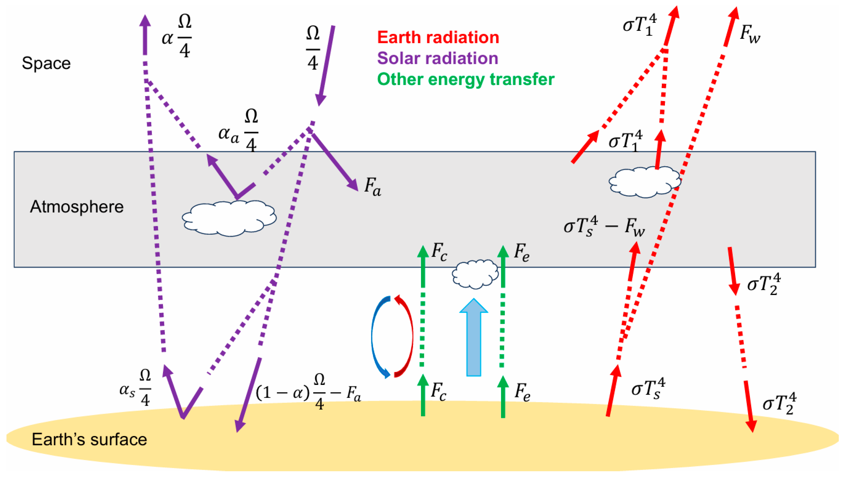
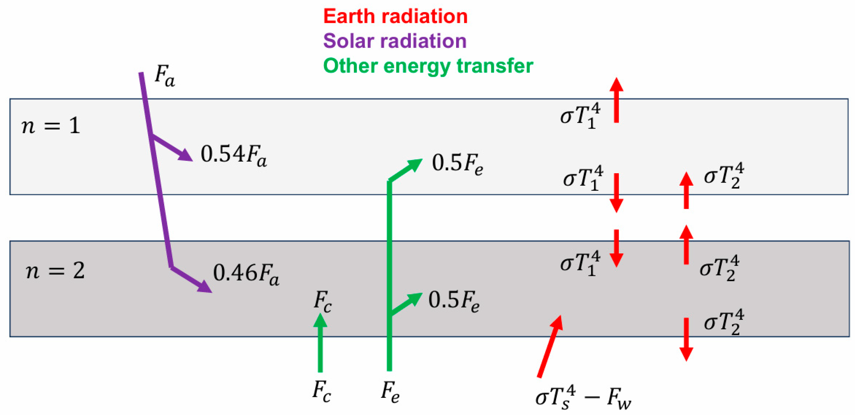
Figure 2 and Figure 3 illustrate a box model composed of a two-layer atmosphere. The numerical values of the parameters shown in the figures are summarized in Table 1. The interior of each layer maintains a constant temperature ( T 1 and T 2 ), and the atmosphere is assumed to be a blackbody. When determining the spatial thickness of each atmospheric layer, the optical thicknesses of the two layers were set equal by ensuring the amount of water vapor contained in the atmosphere is the same in both layers.
The radiation intensity shown in the table refers to the energy carried by electromagnetic waves per unit time and per unit area, with the unit being W/m2. This quantity is also called the radiant energy flux. α represents albedo, indicating the percentage of incident radiation reflected by a material, i.e., its reflectance. The value of α , the Earth’s total albedo, is taken as 0.3 [26]. Of this, three-quarters is attributed to the atmosphere and clouds, and the remainder to the Earth’s surface. Thus, α a and α s are set to 0.3 × (3/4) and 0.3 × (1/4), respectively [30].
F a represents the flux absorbed by the atmosphere and clouds before reaching the Earth’s surface out of the total flux arriving from the Sun. In this study, based on reference [26], approximately 20% of the total flux reaching Earth from the Sun (i.e., Ω / 4 ) is assumed to be absorbed by the atmosphere, setting F a to 68.5 W/m2. The distribution of radiative flux absorbed by the two atmospheric layers is set as 0.54 for Atmosphere 1 and 0.46 for Atmosphere 2. The rationale for this is detailed in Appendix B.
F c represents convective heat transport, specifically sensible heat transport. Within the troposphere, air temperature decreases with increasing altitude. Air masses cooled at higher altitudes become denser and heavier, causing them to gradually descend. Conversely, air masses warmed near the surface gradually ascend. This signifies heat transfer from the surface to the atmosphere, and this heat is denoted as F c . In this study, based on reference [31], this value is set to 20 W/m2. Note that this sensible heat transport occurs in the boundary layer from the surface to an altitude of 100 m and in the mixed layer from there to an altitude of 1 km. Since convection is minimal in the atmosphere above these layers [26], F c is considered only for transport from the surface to the lower atmosphere (Atmosphere 2).
F e represents heat transport associated with the water cycle, specifically latent heat transport. This refers to the energy released into the atmosphere when water evaporated near the surface is transported as water vapor to the upper atmosphere, cooled there, and then liquefies again. In other words, F e signifies the energy transported from near the surface to the upper atmosphere through the gas-liquid phase transition of water. In this study, the value of F e is set to 80 W/m2 [31]. Furthermore, since it is assumed that the two atmospheric layers contain equal amounts of water vapor, F e is distributed equally between Atmospheric Layer 1 and Atmospheric Layer 2.
F w refers to the flux emitted from the Earth’s surface that escapes directly into outer space without being absorbed by the atmosphere. The atmosphere strongly absorbs Earth’s radiation emitted from the surface across nearly all wavelength ranges, with the exception of the 8–12 µm wavelength range, where absorption is weak. It is known that Earth’s radiation in this wavelength range is not significantly absorbed by the atmosphere, and this range is called an atmospheric window [26]. The subscript W in F w originates from “window”. In this study, the value of F w is set to 40 W/m2 [31].
It is noteworthy to clarify whether the concept of an “atmospheric window” and the assumption of the atmosphere as a blackbody can coexist in this model. Theoretically, these two premises are inherently contradictory: a blackbody assumes 100% absorption and emission across all wavelengths, whereas the atmospheric window represents a specific band of transparency (approx. 8–12 micrometers). In this study, we resolve this contradiction by partitioning the radiative flux into two distinct channels. Specifically, the total radiant energy from the surface is divided into (1) a component absorbed by the atmospheric layers (treated as blackbodies) and (2) a component that bypasses the atmosphere through the “window” to be emitted directly into space. By introducing a weighting factor X (the window ratio), we maintain the atmospheric layers as fully absorbing blackbodies while allowing a fraction X of the surface radiation to escape without interaction. For instance, if X = 0.1 , then 10% of the surface radiation is emitted directly to space, while the remaining 90% is absorbed and re-emitted by the blackbody layers. This “energy bifurcation” allows our simple box model to incorporate the effects of the atmospheric window, resulting in surface temperature derivations that are more consistent with observations than those of a standard n -layer model.

4.4. Derivation of the Equation Determining Earth’s Surface Temperature

Taking into account the various energy transfers defined in the previous section, this section derives the equation determining surface air temperature. The balance of fluxes entering and leaving the space, upper atmosphere, and lower atmosphere is described by the following equations, respectively.
Ω 4 = α Ω 4 + σ T 1 4 + F w
2 σ T 1 4 = σ T 2 4 + 0.5 F e + 0.54 F a
2 σ T 2 4 = σ T 1 4 + σ T s 4 + F c + 0.5 F e + 0.46 F a F w
Solving this system of equations for σ T 1 4 , σ T 2 4 , and σ T s 4 yields the following solutions.
σ T 1 4 = 1 α Ω 4 F w
σ T 2 4 = 2 1 α Ω 4 2 F w 0.5 F e 0.54 F a
σ T s 4 = 3 1 α Ω 4 2 F w F c 1.5 F e 1.54 F a
Equation (18) establishes a correlation between surface temperature T s and various forms of energy transfer. Note that this equation has been derived from a two-layer atmospheric box model, which divides the entire atmosphere surrounding the Earth into two layers of equal optical thickness.
By solving the system of Equations (16)–(18) using the constants listed in Table 1, we obtain the values for the upper and lower atmospheric temperatures T 1 and T 2 in addition to the surface temperature T s . These solutions allow us to quantitatively verify that the incoming and outgoing energy fluxes are balanced for the upper atmosphere, lower atmosphere, and the surface, respectively. For reference, a detailed breakdown of these energy fluxes is provided in Appendix C.

4.5. Approximate Representation of the Greenhouse Effect Caused by Increased Water Vapor Content

As previously stated, water vapor demonstrates a pronounced greenhouse effect due to its capacity to absorb Earth’s radiation over a wide spectrum of wavelengths. Consequently, an increase in the amount of water vapor in the atmosphere results in an increase in the overall optical thickness of the atmosphere. In the following discourse, this increase in the optical thickness of the atmosphere (prior to division) due to elevated water vapor content is expressed as an escalation in the number of atmospheric layers post-division. Specifically, this approach maintains the optical thicknesses of atmospheres 1 and 2 as assumed when deriving Equation (18) in the previous section, while adding an additional atmospheric layer possessing the same optical thickness. By making the following modifications to the coefficients of the first and second terms on the right-hand side of Equation (18), we can describe the determination equation for surface temperature T s that accounts for the increased greenhouse effect due to rising water vapor content.
σ T s 4 = n + 1 1 α Ω 4 n F w F c 1.5 F e 1.54 F a
Here, the n contained in the first and second terms on the right-hand side serves as an indicator of the degree to which the greenhouse effect increases. It can generally take values other than integers. For details on the derivation of Equation (19), please refer to Appendix C.
It should be emphasized here that the definition of n will be extended to allow the variable to take not only integer but also real values. This extension is justified as follows. In the present model, the layer number n physically represents the “optical thickness” of the atmosphere, characterized by two primary aspects. First, it serves as an indicator of the greenhouse effect intensity; as n increases, the frequency of absorption and re-emission of surface radiation before reaching space also increases. This effectively simulates the increase in atmospheric optical thickness due to higher greenhouse gas concentrations. Second, n discretizes the vertical temperature structure. Although the actual atmosphere is a continuum, this model represents it as a series of n layers. A larger n thus implies a greater cumulative temperature lapse rate between the surface and the upper atmosphere.
The validity of treating n as a real number stems from the concept of optical thickness. While using integers (e.g., 1 or 2 layers) simplifies the model for intuitive understanding, extending n to a continuous real number redefines it from a discrete “number of layers” to a continuous physical quantity of “atmospheric opacity”. Under this definition, n becomes a continuous variable dependent on greenhouse gas concentration. This extension enables the analysis of gradual climate change, such as quantifying how a subtle increase in greenhouse gases modifies the atmospheric shielding capacity (e.g., to an equivalent of “1.03 layers”).

5. Formulation of Water Vapor Feedback

This section explains the definition and calculation method of the feedback parameter that represents the sign and strength of the feedback (water vapor feedback) associated with an increase in water vapor content. Firstly, the flux F leaving the surface depends on the four physical factors p j   ( 1 j 4 ) , as delineated in Section 3. Concurrently, each of the four factors, p j , depends on T s . These functional relationships can be expressed as follows.
F = f p 1 T S , p 2 T S , p 3 T S , p 4 T S
Using this relation, the feedback parameter λ is defined as follows.
λ = j = 1 4 λ p j ,           λ p j = F p j p j T s
The value of the λ roughly indicates how much the flux F leaving the Earth’s surface changes per 1 K increase in temperature, and its unit is W·m−2·K−1. The sign of the feedback driven by factor p j , denoted by λ p j , is determined by the combination of signs of the two partial derivatives, as illustrated in the second equation of Equation (21). If the two partial derivatives have the same sign, the feedback driven by that factor p j is positive; if they have different signs, the feedback is negative.
This section formulates the partial derivative coefficients p j / T s for the four physical factors p j T s that can drive temperature changes. These four factors are: n , representing the strength of the greenhouse effect; α , the Earth’s albedo; F e , the latent heat flux from the surface to the atmosphere; and F w , the radiative flux emitted through atmospheric windows. The four physical factors under consideration are functions that are dependent solely on the atmospheric water vapor content, denoted by N H 2 O . The atmospheric water vapor content, in turn, is a function that is dependent on the surface temperature, denoted by T s . In the following discussion, therefore, we first derive the relationship linking the change in physical factor p j T s , designated as Δ p j , to the change in water vapor content, denoted as N H 2 O . Next, we derive the relationship between N H 2 O and the change in surface air temperature, indicated by Δ T s . By integrating these two relationships, we determine the four partial derivatives p j / T s contained in the second equation of Equation (21).
(1)
Change in n Expressing the Strength of the Greenhouse Effect
As previously stated, the intensification of the greenhouse effect due to an increase in water vapor content N H 2 O is depicted by a modification in the number of atmospheric layers n in the box model. Below, we assume that n and N H 2 O are proportional. Furthermore, we denote by N H 2 O ( = N H 2 O N H 2 O ( 0 ) ) the change in N H 2 O from its initial value N H 2 O ( 0 ) . Similarly, we denoted by Δ n the change in n from its initial value n 0 caused by N H 2 O . Then we obtain
Δ n n 0 = N H 2 O N H 2 O ( 0 )
To proceed with the discussion using specific numerical values, we define n and N H 2 O below as the changes in n and N H 2 O , respectively, when the surface air temperature is elevated by 1 K from its initial state specified by n 0 and N H 2 O ( 0 ) . The number of atmospheric layers in the initial state, n 0 is set to n 0 = 2.
(2)
Change in Albedo α
Since the majority of Earth’s albedo is due to cloud cover [30], fluctuations in cloud cover give rise to corresponding alterations in Earth’s albedo. Because cloud cover depends on the supply of water vapor from the surface—that is to say, the amount of water vapor in the atmosphere—the albedo α is also influenced by the amount of water vapor.
The fraction ε of the Earth’s surface area covered by clouds is taken as ε = 0.68 [22]. Additionally, the fraction η of Earth’s albedo contributed by clouds is taken as η = 0.75 . Using these constants and performing calculations analogous to those for n , the relative change in α can be expressed as follows.
Δ α α 0 = η ε · N H 2 O N H 2 O ( 0 )
In Equation (23), α 0 denotes the Earth’s albedo prior to an increase in water vapor, designated as the initial state. This parameter is set to α 0 = 0.3.
It is mentioned as a supplement that on Earth, factors other than water vapor content—such as aerosol concentration in the atmosphere, atmospheric stability, and wind speed—also influence albedo [26]. Furthermore, the albedo exhibits a substantial variation between high-level and low-level clouds. Low-level clouds demonstrate a high capacity for reflecting shortwave radiation from the Sun, while high-level clouds do not manifest a discernible absorption band for shortwave radiation [32]. However, for simplification in this study, we assumed that cloud cover is determined solely by atmospheric water vapor content, and differences due to cloud type are not considered.
(3)
Change in Latent Heat Flux F e
Latent heat transport from the surface accompanies the movement of water vapor; therefore, an increase in atmospheric water vapor content leads to an increase in latent heat transport. Using calculations analogous to those performed for n and α , the relative change in F e can be expressed by the following equation.
Δ F e F e , 0 = N H 2 O N H 2 O ( 0 )
The initial value of F e is set to F e , 0 = 80 W/m2, as previously mentioned. Note that in the real Earth, turbulence occurring in the atmosphere also affects latent heat transport [33], but this is ignored in this case.
(4)
Change in Atmospheric Window Emission F w
The atmospheric window refers to the wavelength range of 8–12 µm, where Earth’s radiation absorption by the atmosphere is weak. Nevertheless, even within this wavelength range, increased cloud cover inhibits part of the flux that would otherwise pass directly from the Earth’s surface into space. Therefore, the following section formulates the decrease in F w due to increased cloud cover. Incidentally, high-altitude clouds such as cirrus clouds have a high absorption rate for Earth’s radiation and exhibit a strong greenhouse effect [32]. But for simplification in this paper, cloud cover is considered to depend solely on the amount of water vapor in the atmosphere, and differences in greenhouse effect due to cloud type are ignored.
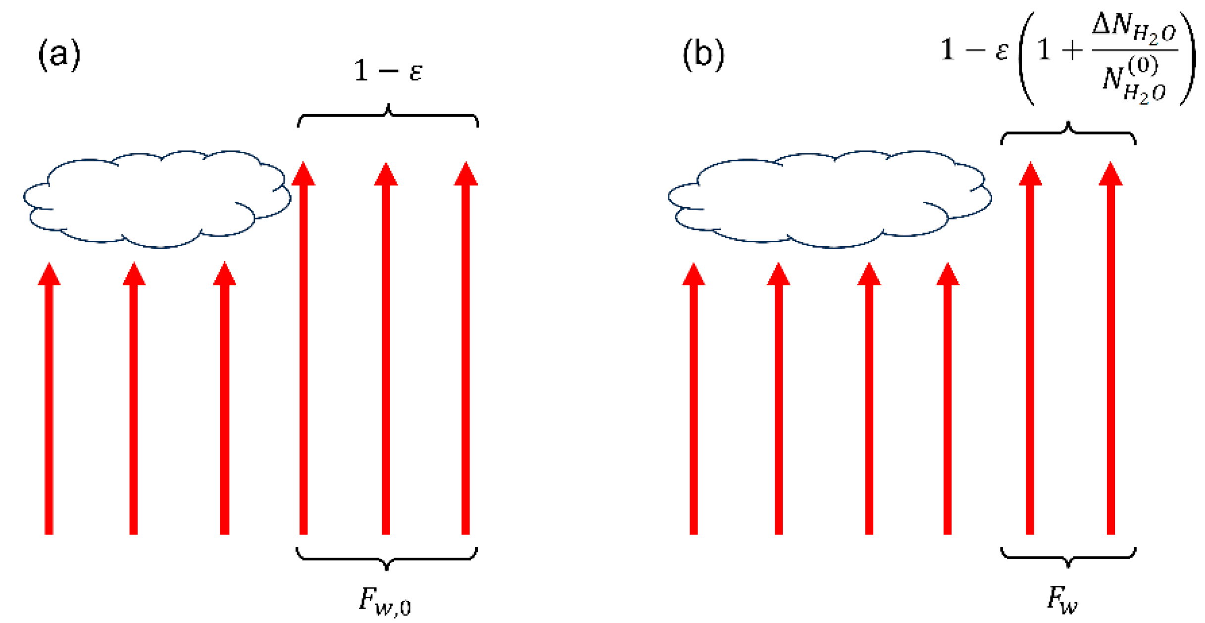
The initial cloud cover fraction ε is set to 0.68, consistent with the previous discussion. Additionally, the initial value of F w is set to F w , 0 = 40 W/m2. Subsequently, we hypothesize that the amount of water vapor will increase as the temperature rises. Assuming a proportional relationship between cloud cover and atmospheric water vapor content, the Earth’s cloud cover ratio after the temperature rise becomes ε 1 + N H 2 O N H 2 O ( 0 ) . Consequently, after the water vapor content increases, F w signifies the radiation that escapes from the Earth’s surface into space through an area encompassing 1 ε 1 + N H 2 O N H 2 O ( 0 ) of the total surface area of the Earth’s atmosphere (see Figure 4). The relationship between the variables can be expressed as follows.
1 ε F w , 0 = 1 ε 1 + N H 2 O N H 2 O ( 0 ) F w
By rearranging the equation using the definition of the derivative, i.e., F w = F w F w , 0 , we obtain
Δ F w F w , 0 = ε 1 ε N H 2 O N H 2 O ( 0 )
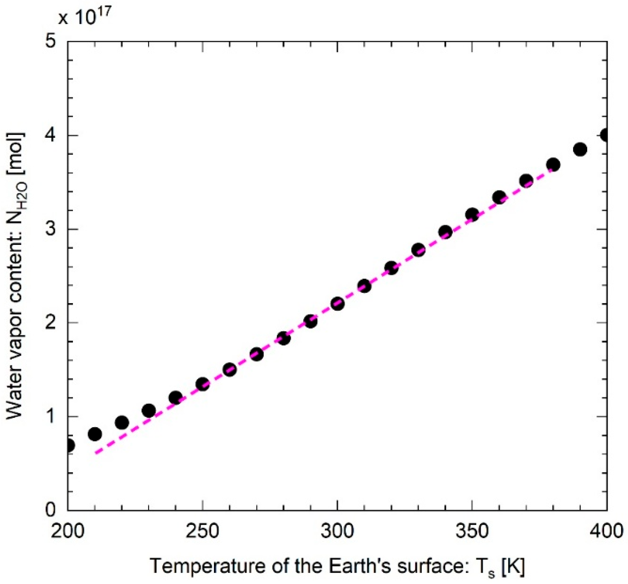
Through the derivations thus far, we have formulated the dependencies of n , α , F e , and F w on N H 2 O . Next, we derive t the relationship linking the change in water vapor content N H 2 O to the change in surface air temperature Δ T s . Figure A3 shows the values of N H 2 O near T s = 295 K, close to the actual Earth’s surface temperature, obtained by numerically integrating the right-hand side of Equation (11). As can be seen from Figure A3, within the temperature range proximate to room temperature, N H 2 O is a linear function of T s , and thus the following equation is applicable.
N H 2 O = N H 2 O T s Δ T s
Now let us redefine the change in N H 2 O when T s increases by 1 K as N H 2 O ; then N H 2 O = N H 2 O / T s , so we obtain the following equation:
p j T s = p j N H 2 O N H 2 O T s Δ p j Δ N H 2 O Δ N H 2 O = Δ p j
This result implies the following representations: n = n T s , α = α T s , F e = F e T s , and F w = F w T s ; it thus follows that:
n T s = n 0 N H 2 O N H 2 O ( 0 )
α T s = α 0 ε η N H 2 O N H 2 O ( 0 )
F e T s = F e , 0 N H 2 O N H 2 O ( 0 )
F w T s = F w , 0 ε · N H 2 O N H 2 O ( 0 ) 1 ε
The partial derivatives F / p j can be readily calculated by rewriting the left-hand side of Equation (19) as F and subsequently taking the partial derivative of both sides as
F n = F w + Ω 4 1 α
F α = Ω 4 n + 1
F F e = 1.5
F F w = n
Using the above results, we can determine the value and sign of the feedback parameter λ p j defined in the second equation of Equation (21).

6. Results

Table 2 presents the numerical results of the eight partial derivatives required to determine the four feedback parameters λ p j . Table 3 summarizes the λ p j values obtained through the proposed model. Within the scope of a simplified two-layer atmospheric model, these numerical results indicate that feedbacks related to the number of atmospheric layers and the atmospheric window are positive, while those stemming from albedo and latent heat act as negative feedbacks.

7. Discussion

This section discusses the validity of the feedback analysis results obtained using a simple two-layer atmospheric box model. The comparison is made with the feedback parameter values listed in the IPCC Sixth Assessment Report [30] (Table 4). The IPCC evaluated these parameters using the three climate model categories: CMIP5 GCMs, CMIP6 ESMs, and AR6 Assessed Ranges [30]. It is important to note that in the IPCC analysis, the radiative flux F is defined as the flux radiated from the top of the atmosphere. Therefore, the feedback parameter values obtained in our present study (where F represents the flux from the Earth’s surface) do not fully match the values published by the IPCC. Nevertheless, comparing the signs and the order of magnitude of the values remains meaningful.
First, the parameter λ n , which represents the water vapor feedback related to the enhanced greenhouse effect in the atmosphere, was estimated from satellite observations to be 1.85 ± 0.32 W·m−2·K−1 [34], while values obtained from CMIP5 and CMIP6 models are 1.77 ± 0.20 W·m−2·K−1 [35]. The value of 2.20 W·m−1·K−1 obtained in the present study is marginally larger than the IPCC-reported values, but the two sets of values are broadly consistent. This finding suggests that even a very simplified two-layer atmospheric box model can reproduce, to some extent, the enhanced greenhouse effect due to increased water vapor.
Next, we consider the feedback parameter λ α , which is associated with increased cloud cover (i.e., increased albedo). The IPCC reports describe the subtropical marine low-level cloud feedback, quantifying its global contribution as 0.14–0.36 W·m−2·K−1 [36]. In contrast, the result obtained in this study is 1.44 W·m−2·K−1. This indicates a mismatch in the sign of the feedback. A possible reason is that the assumption of increased low-level clouds due to global warming may not have been appropriate for quantitative comparison with the IPCC report. The reason for this is briefly noted below.
According to Qu [37] and Kawai [38], two dominant factors have been identified for subtropical low-level clouds. The first is a thermodynamic effect driven by rising sea surface temperatures, which reduces low-level clouds by enhancing the entrainment of dry air into the cloud tops. The second is a stability effect associated with increased inversion layer strength, which in turn increases the low clouds. Fundamentally, these two factors counteract each other. However, the former effect—reducing low-level clouds—is stronger. Consequently, verification using multiple ESM models has shown that as temperatures rise, low-level clouds actually decrease [30].
Thirdly, we consider the feedback parameter λ F e , associated with augmented latent heat transport. The IPCC explains this feedback as the temperature lapse rate feedback, meaning a change in the temperature lapse rate due to increased atmospheric water vapor content [30]. In fact, it has been experimentally observed that the temperature lapse rate tends to decrease as the atmospheric water vapor content increases. For instance, when the atmosphere contains a large amount of water vapor, the cooling of rising air causes the water vapor to condense, releasing latent heat. This released heat suppresses the temperature drop of the air, thereby keeping the temperature lapse rate at a relatively small value. Conversely, when the water vapor content is low, the lack of heat supply from condensation means that the decrease in internal energy due to air expansion leads directly to a drop in air temperature, resulting in a relatively large temperature lapse rate. The IPCC explains the sign and value of the latent heat-related feedback parameter can be attributed to this effect, reporting the average value of this feedback during ongoing global warming being 0.50 ± 0.20 W·m−2·K−1 [35,39,40,41]. Comparing this value, our value of −1.10 W·m−2·K−1 has the same sign but a slightly larger absolute value. If the derivation process could incorporate not only the rate of increase in water vapor content but also the change in the temperature lapse rate due to the atmosphere becoming more humid, it is conceivable that a value closer to those in the cited references could be obtained.
Finally, the feedback parameter λ F w is taken into consideration; it describes the feedback mechanism where increased cirrus clouds absorb outgoing radiation from Earth, which is then re-emitted from the colder upper atmosphere, raising surface temperatures. The IPCC report states that positive feedback exists due to the increase in thin cirrus clouds with low optical thickness in the troposphere-stratosphere boundary layer, with an estimated effect of 0.09 ± 0.09 W·m−2·K−1 [42]. The value we have obtained is 1.56 W·m−2·K−1; this is considerably larger than the result reported in the IPCC document. Possible reasons include overestimating the cloud cover caused by cirrus clouds and overestimating the greenhouse effect from cirrus clouds by assuming that all wavelengths in the atmospheric window region are blocked by cirrus clouds.
It is noteworthy that even the most advanced computer simulation models still have significant margins of error when it comes to feedback related to clouds. The IPCC Sixth Assessment Report presents the combined cloud feedback parameters. For CMIP5 GCMs, the estimated median is 0.41 W·m−2·K−1, with a range of 0.09 to 1.10 W·m−2·K−1. For CMIP6 ESMs, the estimated median is 0.49 W·m−2·K−1, with a range of −0.08 to 1.10 W·m−2·K−1. The AR6 Assessed Ranges demonstrate a central estimate of 0.42 W·m−2·K−1, with a range of 0.10 to 1.94 W·m−2·K−1 [30]. The wide margin of error observed even in the latest research stems from several factors. They include: the cloud formation process involves numerous complex microphysical factors; differences exist in the formation process not only with altitude but also with latitude and land-sea variations; and the role of different cloud types in the greenhouse effect also varies.
This study focused on only two cloud-related factors and aimed to determine feedback parameters using the simplest possible approximation. However, the results differed from previously reported values. Regarding cloud-related factors, even in simplified models, it is considered necessary to incorporate other elements closer to the actual atmosphere before proceeding with the discussion.

8. Conclusions

In this study, we investigated water vapor feedback using a simplified two-layer atmospheric box model. By incorporating only the most essential physical factors and formulating the energy exchange between the two atmospheric layers, outer space, and the Earth’s surface, we constructed an effective equation directly linking atmospheric water vapor content to surface temperature. Calculating the strength and components of the water vapor feedback using this equation yielded results consistent with those obtained from high-precision, high-resolution simulations. Conversely, we found that achieving sufficient quantitative validity for cloud-related factors remains challenging. This issue could potentially be addressed by separately considering the formation processes and greenhouse effects of high-level and low-level clouds.

Author Contributions

Conceptualization, K.M. and H.S.; methodology, K.M. and H.K.; software, K.M.; validation, K.M. and H.S.; formal analysis, K.M. and H.S.; investigation, K.M.; data curation, K.M.; writing—original draft preparation, K.M. and H.S.; writing—review and editing, H.K. and H.S.; visualization, K.M. and H.S.; supervision, H.S. All authors have read and agreed to the published version of the manuscript.

Funding

This work was supported by JSPS KAKENHI Grant Numbers JP24K01111.

Data Availability Statement

The original contributions presented in this study are included in the article. Further inquiries can be directed to the corresponding author.

Conflicts of Interest

The authors declare no conflict of interest.

Appendix A. Discretization of Atmospheric Temperature Distribution

In general, the box model operates under the assumption that the temperature is uniform within each layer. Additionally, it is postulated that the fluxes radiated from the top and bottom of the layer are equal to each other (Figure 2). Equation (11), however, signifies a continuous temperature variation within the layer. To resolve this discrepancy, Appendix A approximates the air temperature distribution as a step function. In the following discussion, the two-layer atmosphere is assumed to have the same optical thickness for Earth’s radiation as it does for shortwave radiation. That is, both layers possess the same capacity to absorb and re-emit radiation.
First, we assume that the amount of water vapor contained within a single atmospheric layer is approximately proportional to its optical thickness for Earth’s radiation. Next, the boundary between Atmospheric Layer 1 and Atmospheric Layer 2 is determined such that the water vapor content is equal. By adjusting the upper limit of the integration range in Equation (11) and calculating the altitude where the water vapor content is half the value at 11,000 m, the boundary between the first and second layers was found to be approximately 1164 m. In other words, the upper atmosphere (Atmosphere 1) is defined as the range from a height h m = 1164 m to h t = 10,000 m, while the lower atmosphere (Atmosphere 2) is defined as the range from the surface h b = 0 m up to a height h m = 1164 m. In light of these findings, the altitude distribution of air temperature is represented by the following step function.
T h = T 2           h b h h m T 1         h m < h h t
The temperatures of the atmospheres are determined by Equations (16) and (17) from the radiative balance model as T 1 = 243.6 K and T 2 = 274.6 K. Additionally, the surface air temperature is calculated in Equation (18) as T s 0 = 288.7 K. This value is proximate to the mean observed surface air temperature of 288 K. Furthermore, Equation (A1) is modified as follows.
T h = T 2 + T s T s 0           h b h h m T 1 + T s T s 0         h m < h h t
The term T s T s 0 corrects for the fact that atmospheric temperature changes in response to changes in surface air temperature.

Appendix B. Layer Dependence of the Radiative Flux Absorption

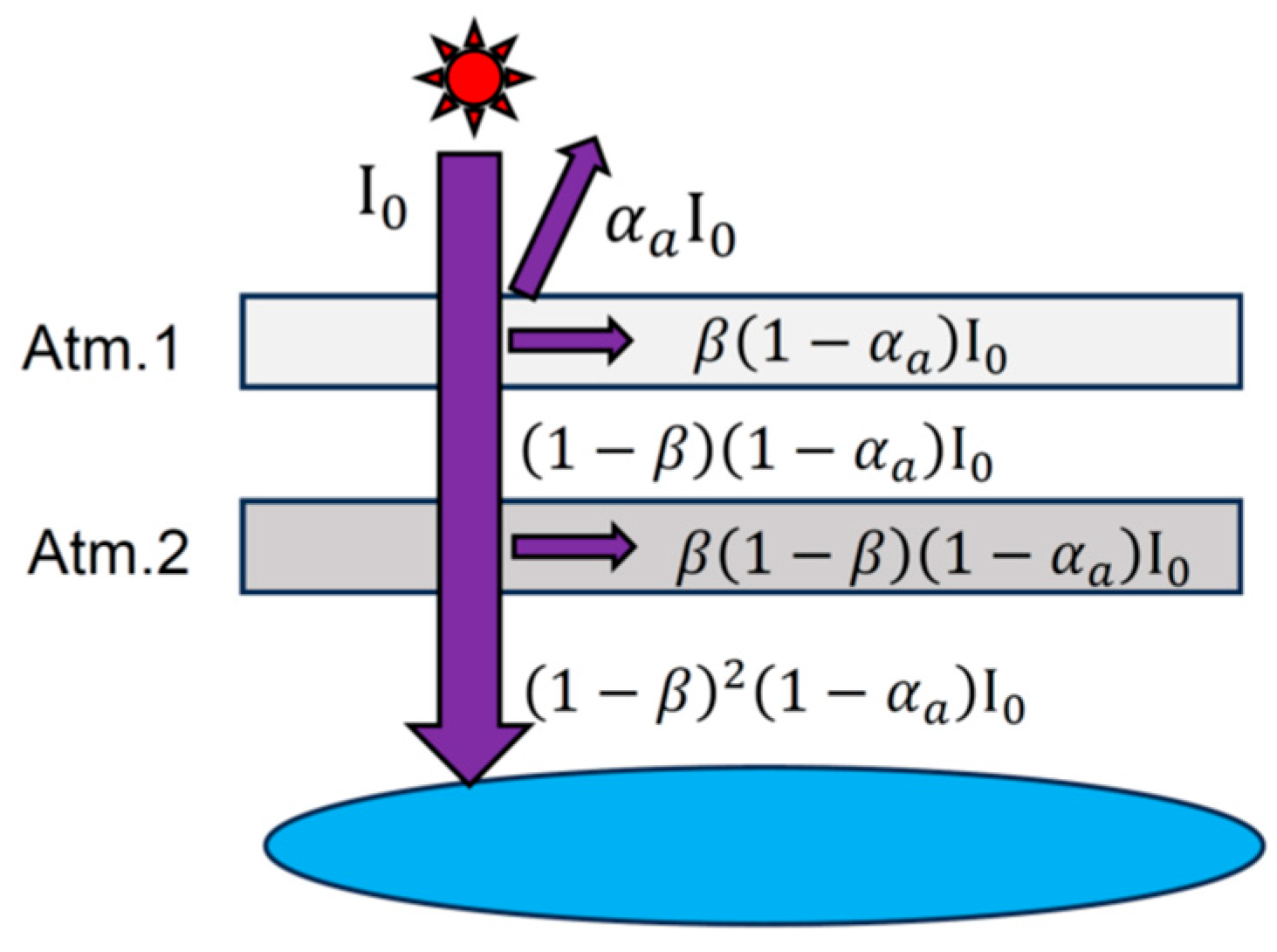
As illustrated in Figure 3, the rationale behind establishing the distribution of radiation flux absorbed by the two atmospheric layers as 0.54 for Atmosphere 1 and 0.46 for Atmosphere 2 is elucidated below.
It has been determined that the radiation emitted from the Sun is of the shortwave variety and thus possesses wavelengths that are shorter in comparison to those emitted from Earth. It is hypothesized that these two atmospheric layers possess equivalent optical thickness for shortwave radiation. Therefore, it can be concluded that the two atmospheres possess equivalent capabilities in terms of shortwave radiation absorption from the Sun. The absorption rate is denoted by β , and for the sake of simplicity, the flux from the Sun is represented as I 0 . Additionally, it is assumed that all reflection of shortwave radiation by the atmosphere occurs at the top of the atmosphere. As illustrated in Figure A1, the reflection of solar radiation at the top of the atmosphere is expressed as α a · I 0 . Consequently, the flux absorbed by atmosphere 1 can be expressed as β 1 α a I 0 . It has been established that only 1 β 1 α a I 0 reaches atmosphere 2, as the remainder is absorbed and attenuated by atmosphere 1. Consequently, despite the fact that atmosphere 2 exhibits an identical absorption rate as atmosphere 1, it absorbs a lesser amount of flux, specifically β 1 β 1 α a I 0 . The flux reaching the ground after passing through these two layers is 1 β 2 1 α a I 0 . This should equal 1 α a I 0 F a . Therefore, if F a = 0.2 I 0 , we can express it as:
1 α a I 0 0.2 I 0 = 1 β 2 1 α a I 0
Solving this equation for β , we obtain β 0.14 .
In this case, the distribution of F a between atmosphere 1 and atmosphere 2 can be expressed as the ratio of the actual amount absorbed by each atmosphere.
β β + β 1 β
β 1 β β + β 1 β  
Substituting the previously obtained β value into the aforementioned equation results in an allocation of 0.54 to Atmosphere 1 and 0.46 to Atmosphere 2. Figure A1 on the right provides a synopsis of the extent of absorption and transmission for solar radiation.
Figure A1. Diagram showing how solar radiation energy from the sun is distributed between two atmospheric layers.
Mmphys 02 00004 g0a1

Appendix C. Radiative Balance at the Two Layers and the Surface

This appendix provides a breakdown of the incoming and outgoing energy fluxes for the upper atmosphere, the lower atmosphere, and the surface, based on initial values prior to the increase in atmospheric water vapor (see Figure 2). All values are expressed in W/m2. It can be confirmed that the incoming and outgoing energy amounts are perfectly balanced across both atmospheric layers and the surface.
  • Radiative Equilibrium at the Upper Atmosphere (All units are in W/m2):
(i)
Incoming energy flux to the upper atmosphere:
-
Supply from the lower atmosphere σ T 2 4 : 322.51
-
Solar radiation absorbed by the upper atmosphere 0.54 F a : 36.99
-
Latent heat transport 0.5 F e : 40
Total: 399.5
(ii)
Outgoing energy flux from the upper atmosphere:
-
Downward radiation σ T 1 4 : 199.75
-
Upward radiation σ T 1 4 : 199.75
Total: 399.5
2.
Radiative Equilibrium at the Lower Atmosphere (All units are in W/m2)
(i)
Incoming energy flux to the lower atmosphere:
-
Solar radiation absorbed by the lower atmosphere 0.46 F a : 31.51
-
Radiation from the surface absorbed by the lower atmosphere σ T s 4 F w : 353.76
-
Supply from the upper atmosphere σ T s 4 : 199.75
-
Latent heat transport 0.5 F e : 40
-
Sensible heat transport F c : 20
Total: 645.02
(ii)
Outgoing energy flux from the lower atmosphere:
-
Downward radiation σ T 2 4 : 322.51
-
Upward radiation σ T 2 4 : 322.51
Total: 645.02
3.
Radiative Equilibrium at the Earth’s surface: (All units are in W/m2)
(i)
Incoming energy flux to the surface:
-
Direct solar radiation transmitted through the atmosphere 1 α Ω 4 F a : 171.25
-
Supply from the lower atmosphere σ T 2 4 : 322.51
Total: 493.76
(ii)
Outgoing energy flux from the surface:
-
Radiation from the surface σ T s 4 : 393.76
-
Latent heat transport F e : 80
-
Sensible heat transport F c : 20
Total: 493.76

Appendix D. Derivation of Equation (19)

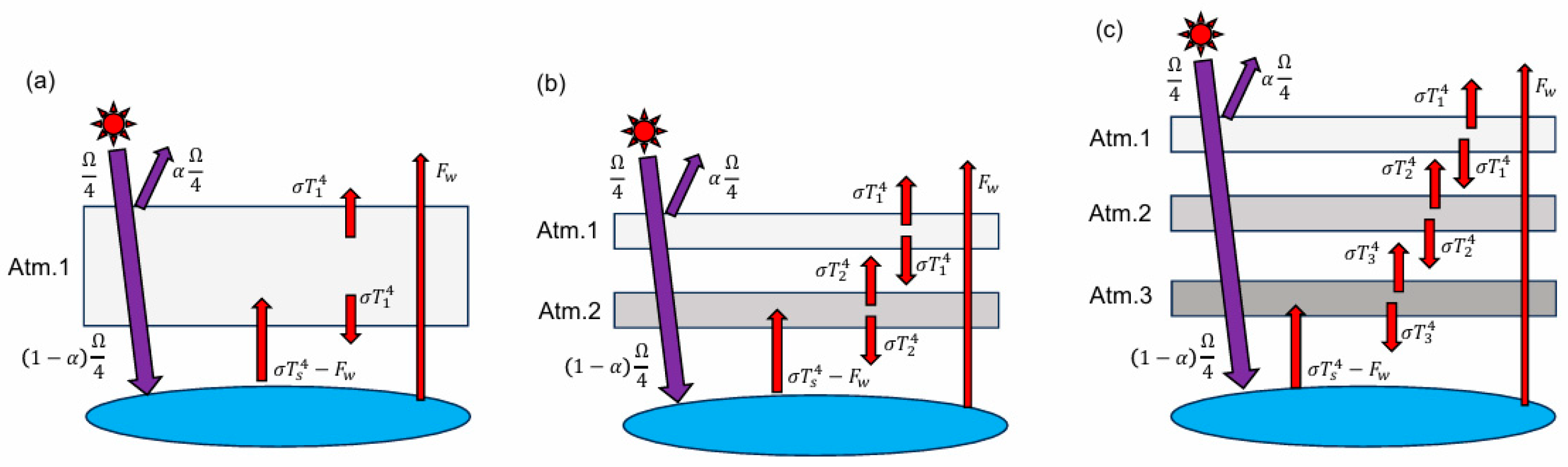
This Appendix explains how the atmospheric layer number n is incorporated into Equation (18). For each of the three n -layer atmospheric box models ( n = 1,2 , 3 ) depicted in Figure A2, we consider the fluxes exchanged between space and the n -layer atmosphere. In the following discussion, the effects of latent heat flux F e , sensible heat flux F c , and atmospheric solar radiation absorption F a are all neglected (even if these terms were included, they would only act as constant terms, thus having no impact on the subsequent discussion and leaving the conclusion unchanged).
Figure A2. Simplified n-layered atmospheric model: (a) n = 1, (b) n = 2, (c) n = 3.
Mmphys 02 00004 g0a2
For n = 1 , we obtain the following result:
Ω 4 = α Ω 4 + σ T 1 4 + F w
2 σ T 1 4 = σ T s 4 F w
For n = 2 , we obtain the following result:
Ω 4 = α Ω 4 + σ T 1 4 + F w
2 σ T 1 4 = σ T 2 4
2 σ T 2 4 = σ T 1 4 + σ T s 4 F w
For n = 3 , we obtain the following result:
Ω 4 = α Ω 4 + σ T 1 4 + F w
2 σ T 1 4 = σ T 2 4
2 σ T 2 4 = σ T 1 4 + σ T 3 4
2 σ T 3 4 = σ T 2 4 + σ T s 4 F w
The results of solving these three sets of simultaneous equations for σ T s 4 and σ T i 4   ( 1 i n ) , respectively, are summarized in Table A1.
Table A1. List of solutions to the simultaneous equations for the n-layer atmospheric models (n = 1, 2, 3).
1-Layer Atm.2-Layer Atm.3-Layer Atm.
σ T 1 4 1 α Ω 4 F w 1 α Ω 4 F w 1 α Ω 4 F w
σ T 2 4 2 1 α Ω 4 2 F w 2 1 α Ω 4 2 F w
σ T 3 4 3 1 α Ω 4 3 F w
σ T s 4 2 1 α Ω 4 F w 3 1 α Ω 4 2 F w 4 1 α Ω 4 3 F w
As indicated by the findings presented in Table A1, σ T n 4 and σ T s 4 for an n -layer atmosphere can be expressed as follows:
σ T n 4 = n 1 α Ω 4 n F w
σ T s 4 = n + 1 1 α Ω 4 n F w
In fact, it can be easily proven that the above two equations hold for general values of n even when n is increased to 4 or higher. Furthermore, let us reintroduce the effects of latent heat transport F e , sensible heat transport F c , and atmospheric solar radiation absorption F a —which we ignored in the preceding discussion—into the right-hand side of Equation (A16) we derived above. We then find that when the increase in greenhouse gases is expressed as an increase in the number of layers n , Equation (18) can be extended as follows (Equation (19) in the main text).
σ T s 4 = n + 1 1 α Ω 4 n F w F c 1.5 F e 1.54 F a

Appendix E. Integration Result of Equation (11)

The results of numerically evaluating the integral shown in Equation (11) of the main text are presented in Figure A3. The graph exhibits almost linear behavior within the temperature range close to the actual surface temperature of the Earth ( 290 K).
Figure A3. Relation between the water vapor content in the whole atmosphere and the Earth’s surface temperature.
Mmphys 02 00004 g0a3

References

  1. Manabe, S.; Stricker, R.H. Thermal Equilibrium of the Atmosphere with a Convective Adjustment. J. Atmos. Sci. 1964, 21, 361–385. [Google Scholar] [CrossRef] [Scilit]
  2. Manabe, S.; Bryan, K. Climate Calculations with a Combined Ocean-Atmosphere Model. J. Atmos. Sci. 1969, 21, 786–789. [Google Scholar] [CrossRef] [Scilit]
  3. Manabe, S. Role of greenhouse gas in climate change. Tellus A Dyn. Meteorol. Oceanogr. 2019, 71, 1620078. [Google Scholar] [CrossRef] [Scilit]
  4. Alizadeh, O. Advances and challenges in climate modeling. Clim. Change 2022, 170, 18. [Google Scholar] [CrossRef] [Scilit]
  5. Fuhrer, O.; Chadha, T.; Hoefler, T.; Kwasniewski, G.; Lapillonne, X.; Leutwyler, D.; Lüthi, D.; Osuna, C.; Schär, C.; Schulthess, T.C.; et al. Near-global climate simulation at 1 km resolution: Establishing a performance baseline on 4888 GPUs with COSMO 5.0. Geosci. Model Dev. 2018, 11, 1665–1681. [Google Scholar] [CrossRef] [Scilit]
  6. Eyring, V.; Bony, S.; Meehl, G.A.; Senior, C.A.; Stevens, B.; Stouffer, R.J.; Taylor, K.E. Overview of the Coupled Model Intercomparison Project Phase 6 (CMIP6) experimental design and organization. Geosci. Model Dev. 2016, 9, 1937–1958. [Google Scholar] [CrossRef] [Scilit]
  7. Zeng, X. Atmospheric Instability and Its Associated Oscillations in the Tropics. Atmosphere 2023, 14, 433. [Google Scholar] [CrossRef] [Scilit]
  8. Hartmann, D.L.; Blossey, P.N.; Dygert, B.D. Convection and Climate: What Have We Learned from Simple Models and Simplified Settings? Curr. Clim. Change Rep. 2019, 5, 196–206. [Google Scholar] [CrossRef] [Scilit]
  9. Liu, Y.; Yao, X.; Zhou, L.; Ming, T.; Li, W.; de Richter, R. Removal of Atmospheric Methane by Increasing Hydroxyl Radicals via a Water Vapor Enhancement Strategy. Atmosphere 2024, 15, 1046. [Google Scholar] [CrossRef] [Scilit]
  10. Zhou, X.; Cheng, Y.; Liu, L.; Huang, Y.; Sun, H. Significant Increases in Water Vapor Pressure Correspond with Climate Warming Globally. Water 2023, 15, 3219. [Google Scholar] [CrossRef] [Scilit]
  11. Seeley, L.H. Tutorials in climate modeling. Am. J. Phys. 2023, 91, 690–695. [Google Scholar] [CrossRef] [Scilit]
  12. Olbers, D.; Willebrand, J.; Eden, C. Ocean Dynamics; Springer: Berlin/Heidelberg, Germany, 2012. [Google Scholar]
  13. Canadell, J.G.; Monteiro, P.M.; Costa, M.H.; Da Cunha, L.C.; Cox, P.M.; Eliseev, A.V.; Henson, S.; Ishii, M.; Jaccard, S.; Koven, C. Global Carbon and Other Biogeochemical Cycles and Feedbacks. In IPCC Sixth Assessment Report; Cambridge University Press: Cambridge, UK, 2023; pp. 673–816. [Google Scholar] [CrossRef] [Scilit]
  14. Begon, M.; Townsend, C.R.; Harper, J.L. Ecology: From Individuals to Ecosystems; Wiley-Blackwell: Hoboken, NJ, USA, 2005. [Google Scholar]
  15. Chapin, F.S.; Matson, P.A.; Vitousek, P.M. Principles of Terrestrial Ecosystem Ecology; Springer: Berlin/Heidelberg, Germany, 2002. [Google Scholar]
  16. Goody, R.M.; Walker, J.C.G. ATMOSPHERES (Foundations of Earth Science Series); Prentice-Hall: Upper Saddle River, NJ, USA, 1972. [Google Scholar]
  17. Manabe, S.; Wetherald, R.T. Thermal Equilibrium of the Atmosphere with a Given Distribution of Relative Humidity. J. Atmos. Sci. 1967, 24, 241–259. [Google Scholar] [CrossRef] [Scilit]
  18. Kiehl, J.T.; Trenberth, K.E. Earth’s Annual Global Mean Energy Budget. Bull. Am. Meteorol. Soc. 1997, 78, 197–208. [Google Scholar] [CrossRef] [Scilit]
  19. Randall, D.A.; Wood, R.A.; Bony, S.; Colman, R.; Fichefet, T.; Fyfe, J.; Kattsov, V.; Pitman, A.; Shukla, J.; Srinivasan, J.; et al. Climate Models and Their Evaluation. In IPCC WG1 Fourth Assessment Report: Climate Change 2007; Cambridge University Press: Cambridge, UK, 2007; Chapter 8. [Google Scholar]
  20. Sherwood, S.C.; Dixit, V.; Salomez, C. The global warming potential of near surface emitted water vapour. Environ. Res. Lett. 2018, 13, 104006. [Google Scholar] [CrossRef] [Scilit]
  21. Xue, J.; Yuan, C.; Qu, Y.; Huang, Y. Observation of Multilayer Clouds and Their Climate Effects: A Review. Atmosphere 2025, 16, 692. [Google Scholar] [CrossRef] [Scilit]
  22. Stubenrauch, C.J.; Rossow, W.B.; Kinne, S.; Ackerman, S.; Cesana, G.; Chepfer, H.; Di Girolamo, L.; Getzewich, B.; Guignard, A.; Heidinger, A.; et al. Assessment of Global Cloud Datasets from Satellites: Project and Database Initiated by the GEWEX Radiation Panel. Bull. Am. Meteorol. Soc. 2013, 94, 1031–1049. [Google Scholar] [CrossRef] [Scilit]
  23. Inoue, T. On the Temperature and Effective Emissivity Determination of Semi-Transparent Cirrus Clouds by Bi-Spectral Measurements in the 10 µm Window Region. J. Meteorol. Soc. Jpn. Ser. II 1985, 63, 88–99. [Google Scholar] [CrossRef] [Scilit]
  24. National Astronomical Observatory of Japan. Handbook of Scientific Tables; National Astronomical Observatory of Japan: Maruzen, Japan, 2025. [Google Scholar] [CrossRef] [Scilit]
  25. Schoeberl, M.R.; Jensen, E.J.; Pfister, L.; Ueyama, R.; Wang, T.; Selkirk, H.; Avery, M.; Thornberry, T.; Dessler, A.E. Water Vapor, Clouds, and Saturation in the Tropical Tropopause Layer. J. Geophys. Res. Atmos. 2019, 124, 3984–4003. [Google Scholar] [CrossRef] [Scilit] [PubMed]
  26. Wallace, J.M.; Hobbs, P.V. Atmospheric Science: An Introductory Survey; Academic Press: San Diego, CA, USA, 1977. [Google Scholar]
  27. Dalal, M. A Textbook of Physical Chemistry—Volume 1; Dalal Institute: Rohtak, India, 2018. [Google Scholar]
  28. International Telecommunication Union, Radiocommunication Sector (ITU-R). Recommendation ITU-R P.835-5: Reference Standard Atmospheres, P Series: Radiowave Propagation. 2012. Available online: https://www.itu.int/rec/R-REC-P.835-6-201712-S/en (accessed on 24 December 2025).
  29. Ingram, W. A very simple model for the water vapour feedback on climate change. Q. J. R. Meteorol. Soc. 2010, 136, 30–40. [Google Scholar] [CrossRef] [Scilit]
  30. Armour, K.; Forster, P.; Storelvmo, T.; Collins, W.; Dufresne, J.L.; Frame, D.; Lunt, D.; Mauritsen, T.; Palmer, M.; Watanabe, M.; et al. The Earth’s Energy Budget, Climate Feedbacks and Climate Sensitivity. In IPCC Sixth Assessment Report; Cambridge University Press: Cambridge, UK, 2023; pp. 923–1055. [Google Scholar] [CrossRef] [Scilit]
  31. My NASA Data, Earth’s Energy Budget. 2022. Available online: https://mynasadata.larc.nasa.gov/basic-page/earths-energy-budget (accessed on 24 December 2025).
  32. Hayasaka, T. Fundamentals of Cloud Radiative Properties. Low Temp. Sci. 2014, 72, 145–150. Available online: http://id.ndl.go.jp/bib/025499641 (accessed on 24 December 2025). (In Japanese)
  33. Lee, X. Fundamentals of Boundary-Layer Meteorology; Springer Atmospheric Sciences: London, UK, 2018. [Google Scholar]
  34. Liu, R.; Su, H.; Liou, K.-N.; Jiang, J.H.; Gu, Y.; Liu, S.C.; Shiu, C.-J. An Assessment of Tropospheric Water Vapor Feedback Using Radiative Kernels. J. Geophys. Res. Atmos. 2018, 123, 1499–1509. [Google Scholar] [CrossRef] [Scilit]
  35. Zelinka, M.D.; Myers, T.A.; McCoy, D.T.; Po-Chedley, S.; Caldwell, P.M.; Ceppi, P.; Klein, S.A.; Taylor, K.E. Causes of higher climate sensitivity in CMIP6 models. Geophys. Res. Lett. 2020, 46, e2019GL085782. [Google Scholar] [CrossRef] [Scilit]
  36. Klein, S.A.; Hall, A.; Norris, J.R.; Pincus, R. Low-cloud feedbacks from cloud-controlling factors: A review. Surv. Geophys. 2017, 38, 1307–1329. [Google Scholar] [CrossRef] [Scilit]
  37. Qu, X.; Hall, A.; Klein, S.A.; DeAngelis, A.M. Positive tropical marine low cloud cover feedback inferred from cloud-controlling factors. Geophys. Res. Lett. 2015, 42, 7767–7775. [Google Scholar] [CrossRef] [Scilit]
  38. Kawai, H.; Koshiro, T.; Webb, M.J. Interpretation of Factors Controlling Low Cloud Cover and Low Cloud Feedback Using a Unified Predictive Index. J. Clim. 2017, 30, 9119–9131. [Google Scholar] [CrossRef] [Scilit]
  39. Dessler, A.E. Observations of Climate Feedbacks over 2000–2010 and Comparisons to Climate Models. J. Clim. 2013, 26, 333–342. [Google Scholar] [CrossRef] [Scilit]
  40. Caldwell, P.M.; Zelinka, M.D.; Taylor, K.E.; Marvel, K. Quantifying the sources of intermodel spread in equilibrium climate sensitivity. J. Clim. 2016, 29, 513–524. [Google Scholar] [CrossRef] [Scilit]
  41. Colman, R.A.; Hanson, L. On the relative strength of radiative feedbacks under climate variability and change. Clim. Dyn. 2017, 49, 2115–2129. [Google Scholar] [CrossRef] [Scilit]
  42. Zhou, C.; Dessler, A.E.; Zelinka, M.D.; Yang, P.; Wang, T. Cirrus feedback on interannual climate fluctuations. Geophys. Res. Lett. 2014, 41, 9166–9173. [Google Scholar] [CrossRef] [Scilit]
Figure 1. Actual measurement data of relative humidity distribution with altitude change [28] and the fitting curve using cubic polynomial approximation expressed by Equation (8).
Mmphys 02 00004 g001
Figure 2. Schematic illustration of the two-layer radiation balance model. Energy transfer between the space, atmosphere, and the Earth’s surface is demonstrated.
Mmphys 02 00004 g002
Figure 3. Energy transfer occurring between the upper and lower atmospheric layers.
Mmphys 02 00004 g003
Figure 4. (a) Atmospheric state with cloud cover ε at the initial state. Since the proportion 1 ε of the total atmospheric area is a cloud-free region, surface radiation F w , 0 escapes into outer space through this gap. (b) Atmospheric state where cloud cover increases due to rising water vapor content. As water vapor increases, the area of the cloud-free region decreases.
Mmphys 02 00004 g004
Table 1. Lists of parameter values applied to the two-layer atmospheric box model.
Ω Intensity of solar radiation reaching Earth1370 W/m2
σ Stefan-Boltzmann constant5.67 × 10−8 W/(m2·K4)
α Earth’s total albedo0.3
α a Albedo due to the atmosphere and clouds0.225
α s Albedo due to the surface0.075
T s Surface temperature
T 1 Upper atmosphere temperature
T 2 Lower atmospheric temperature
F a Solar radiation absorbed by the atmosphere68.5 W/m2
F c Heat transport by convection (sensible heat transport)20 W/m2
F e Heat transport by water cycle (latent heat transport)80 W/m2
F w Radiation escaping directly into space from the surface40 W/m2
Table 2. The values of each partial derivative coefficient characterizing the strength of water vapor feedback.
n T s α T s F e T s F w T s F n F α F F e F F w
K−1K−1W·m−2·K−1W·m−2·K−1W·m−2W·m−2
1.10 × 10 2 1.40 × 10 3 0.73 0.78 199.75 1027.5 1.50 2.00
Table 3. Results of the feedback parameter values (W·m−2·K−1).
λ n λ α λ F e λ F w
2.20 1.44 1.10 1.56
Table 4. Comparison of our results with the IPCC Report (W·m−2·K−1).
λ n λ α λ F e λ F w
Our results 2.20 1.44 1.10 1.56
IPCC Report 1.77 ± 0.20 0.25 ± 0.11 0.50 ± 0.20 0.09 ± 0.09
Disclaimer/Publisher’s Note: The statements, opinions and data contained in all publications are solely those of the individual author(s) and contributor(s) and not of MDPI and/or the editor(s). MDPI and/or the editor(s) disclaim responsibility for any injury to people or property resulting from any ideas, methods, instructions or products referred to in the content.