Intelligent Optimal Strategy for Balancing Safety–Quality–Efficiency–Cost in Massive Concrete Construction

Abstract

Thermal stress control is crucial for massive concrete structures during construction. The cooling strategies directly determine the safety of structures, material quality, construction efficiency, and project cost. However, precise spatiotemporal thermal stress regulation and management are difficult to achieve due to the lack of balanced discriminant criteria and multi-objective optimization methods for the selection of traditional strategies. Therefore, an intelligent optimization method for thermal stress management strategy in massive concrete structures, considering the balance of safety, quality, efficiency, and cost (SEQC-TSOM), is proposed. Initially, a Thermal Stress Simulation Mechanism Model (TSSM) is constructed to accurately evaluate the structural state throughout the entire process. Subsequently, a mechanism data-driven surrogate model (MD-SM) is constructed to quickly evaluate the structural response under different cooling strategies. Furthermore, a multi-objective intelligent optimization model and a multi-criteria decision-making model are proposed to filter the intelligent optimal strategy from the Pareto solution set. Finally, a case study based on the Baihetan arch dam project is conducted, and the results show that the safety, quality, efficiency, and cost (SEQC)-balanced strategy increases safety by 42%, improves cooling efficiency by 36%, and reduces cooling costs by 20.6% compared with traditional strategies.

1. Introduction

Temperature-induced cracks have a significant impact on the safety of concrete structures during both construction and operation, especially for massive concrete structures such as dams, nuclear power plant-containment structures, bridge piers, and lock piers [1,2,3,4,5]. Post-cooling systems serve as highly effective means of actively controlling stress, and the cooling strategies directly determine the safety of mass concrete structures, material quality, construction efficiency, and project cost [1,6,7]. The cracking mechanism of massive concrete structures under temperature load is complex. Therefore, the design of cooling strategies must take into account the thermodynamic properties of materials, structural degree of restraint characteristics, construction processes, boundary conditions, and the impact of cooling systems. However, due to the absence of balanced discriminative criteria and multi-objective intelligent optimization methods, conventional cooling strategies demonstrate imbalances in terms of safety, quality, efficiency, and cost. Therefore, it is crucial to investigate a mechanism data-driven multi-objective intelligent optimization method for temperature stress and offer SEQC-balanced cooling strategies for engineering purposes. This will enable precise control and management of temporal–spatial thermal stress of massive concrete structures, as is essential for achieving the goals of safe, high-quality, efficient, and cost-effective intelligent construction.

The deformation caused by temperature changes under restraints leads to thermal stress in massive concrete structures, resulting in the formation of temperature-induced cracks. Therefore, research on the failure mechanism of thermal loading primarily focuses on four aspects: thermodynamic properties, mechanical performance under temperature influence, failure behavior, and failure criteria under temperature-restraint interaction. From a microscopic perspective, a significant amount of hydration heat is released with the generation of hydration products such as calcium silicate hydrate (C-S-H), calcium hydroxide (C-H), Aluminate-Ferrite-tri (AFt), and Aluminate-Ferrite-mono (AFm), leading to an increase in the internal temperature of the concrete [8]. Scholars have quantitatively studied the thermal properties of different cement components and their hydration products, including thermal conductivity, linear expansion coefficient, and specific heat capacity. Among them, the proportion of tricalcium silicate (C3S) and dicalcium silicate (C2S) has the greatest influence on hydration heat [9]. Therefore, Wang et al. produced low-heat cement by adjusting the proportion of C3S and C2S, which can reduce the difficulty in controlling temperature in massive concrete [10]. From a macroscopic perspective, scholars have conducted quantitative research on the linear expansion coefficient, strength, elastic modulus, creep, and relaxation characteristics of massive concrete under different curing conditions through adiabatic temperature rise tests, isothermal calorimetry, thermogravimetric analysis, and strength testing methods [11]. Among them, the linear expansion coefficient and creep characteristics are crucial for the evolution of structural stress. In order to more accurately evaluate the failure behavior of concrete under the combined effect of temperature and restraint, scholars have developed advanced variable-restraint temperature stress testing machines [12,13,14]. In particular, Zhu et al. developed a multi-machine temperature stress testing system based on an artificial climate laboratory, which enables the obtainment of thermodynamic properties such as coefficient of thermal expansion, elastic modulus, creep relaxation, and tensile strength through multiple devices in a single test [15]. In addition, for the failure criterion in complex loading processes of massive concrete, various criteria have been proposed, including the maximum tensile stress criterion, maximum tensile strain criterion, stress-and-strain-based failure criteria [16], and energy-based criteria [17]. In summary, research on the cracking mechanism caused by temperature loading is crucial for assessing safety, and the models for thermodynamic properties and failure criteria provide an important basis for regulating thermal stress.

The evolution of temperature stress exhibits characteristics such as nonlinearity, time-dependence, and accumulation. Accurately assessing structural stress serves as the foundation for stress management. However, there are numerous factors influencing temperature stress in massive concrete structures, including the thermodynamic properties of materials, structural forms, construction sequences, and boundary conditions. Moreover, measuring stress in actual structures poses challenges. As a result, scholars have utilized the finite element method to conduct thermomechanical-coupled analyses of massive concrete structures, such as dams, containment structures, and bridge piers [18]. Due to the wide temperature range (usually ranging from 10 to 40 °C) and long cooling periods (requiring hundreds of years to reach stable temperatures) in massive concrete structures, temperature field simulation analysis is divided into two categories: the construction phase and the operational phase. Notably, temperature-induced cracks predominantly occur during the construction phase. To mitigate this, scholars have systematically studied concrete casting temperature, adiabatic temperature rise, cooling system effectiveness, and surface insulation measures to avoid temperature-induced cracks on the surface and inside the structure [19,20,21,22]. Additionally, researchers have conducted operational-phase temperature field analyses for structures such as dams in complex service environments, focusing on the effects of solar radiation, reservoir water temperature [22], and periodic temperature changes [23] on temperature and stress fields. The creep effect of massive concrete cannot be neglected during both the construction and operational phases. Creep is significantly influenced by material composition, degree of hydration, age, and load level, and it has a notable effect on adjusting structural stress. On the one hand, during the early age of concrete when the temperature increases, early-age creep can relax 20–50% of compressive stress [12], ultimately leading to an increase in tensile stress. Therefore, various models for early-age creep have been proposed [1,24]. On the other hand, although creep can reduce stress levels, it also causes material strength to be reduced by 10–40% due to the high stress levels during the operational phase, thereby increasing the risk of cracking [16]. Thus, creep effects must be considered in the analysis of temperature stress in massive concrete structures. Under constrained conditions, the autogenous shrinkage of concrete induces additional restraint stresses, particularly for concrete with a water–cement ratio less than 0.5. Models such as the CEB-FIB, RILEM, Tazawa, and B4 [25] have been utilized to predict concrete autogenous shrinkage. Therefore, in addition to thermal deformation and creep, the analysis of mechanisms must also consider the effects of autogenous volume deformation. In conclusion, the finite element method provides a means for accurate analysis of temperature stress in structures. However, considering the complexity of construction in massive concrete structures, the efficiency of simulating temperature stress throughout the entire process is low and cannot meet the demand for optimized time–space cooling strategies.

Cooling systems are essential for managing thermal stress. In the context of massive concrete, temperature control typically entails pre-cooling and post-cooling techniques. Pre-cooling aims to reduce the pouring temperature and effectively manage the maximum temperature, often achieved through the utilization of cooling aggregates and cold water mixing. Conversely, post-cooling involves controlling the temperature of the concrete after pouring by employing cooling water pipes. The utilization of a cooling water circulation system was initially introduced by the U.S. Bureau of Reclamation during the construction of the Owyhee Dam, and it was subsequently extended to the Hoover Dam, successfully mitigating the occurrence of temperature-induced cracks [26]. Over the course of nearly a century of application, the effectiveness of cooling water circulation in stress control has been firmly established. Research on cooling water circulation systems primarily falls into two categories: experimental investigation of the underlying mechanisms and numerical simulation. Scholars have conducted experiments to examine the composition, materials of the pipes, and layout of the cooling water circulation system, while also evaluating the influence of cooling water flow rate, temperature, time, and water pressure on the cooling efficiency [6,7]. Furthermore, scholars have pursued research on equivalent and fine-scale numerical simulation of cooling water pipes. With regard to equivalent simulation, various methods have been proposed, including the equivalent heat conduction method (EHCM) [27] and the method based on equivalent surfaces [20]. In terms of fine-scale simulation, three-dimensional discrete finite element simulation methods [28], double-layer staggered heterogeneous cooling water pipe simulation methods [29], composite element methods [30], localized radial basis function collocation methods [29], and thermal–fluid coupling models (HFCMs) [31] have been proposed. Although fine simulation methods can effectively evaluate temperature gradients around cooling water pipes, the scale of computation grids is too large to be used for rapid stress evaluation of large structures. The equivalent cooling method is more suitable for engineering applications. In addition, ACI and RILEM provide recommendations for the application of cooling water pipes [32,33]. Despite the development of many automated cooling systems [34,35], developing reasonable cooling system strategies remains crucial for thermal stress management. Unfortunately, strategy research is rare, especially for complex and massive concrete structures. For example, an arch dam comprises thousands of pouring units, and each unit would require years for natural cooling. The interval between arch dam pours is merely 7–10 days, a timeframe that is insufficient for allowing adequate free heat dissipation. Hence, controlled cooling water circulation is imperative to manage the temperature gradient, with each casting unit requiring up to two months of temperature control to reach a stable temperature. Additionally, transverse joint grouting is an essential prerequisite for the arch dam to function as an integral structure. Cooling must be finalized before grouting, which imposes stringent requirements on the efficiency of the cooling process and the safety during rapid temperature reduction. From this, it is evident that controlled cooling of large volume concrete is vitally necessary, and the cooling strategy has a significant impact on safety and efficiency, thus there is a practical demand for optimizing cooling strategies in engineering projects.

From the perspective of project management, the selection of cooling strategies can be regarded as a multi-objective optimization problem of time, cost, and quality tradeoff (TCQT). However, due to the requirements of structural safety, cooling strategies need to simultaneously satisfy the balance of safety, quality, efficiency, and cost. This makes the multi-objective optimization problem more complex, especially in terms of accuracy and efficiency. Therefore, accurate and efficient performance evaluation surrogate models, efficient swarm intelligence optimization algorithms, and multi-criteria decision-making methods are crucial. With the rise of artificial intelligence technologies such as machine learning and swarm intelligence optimization algorithms, surrogate models have been widely applied in structural parameter inversion [36], deformation prediction [37], material performance prediction [38,39], and other areas. Currently, there are three main forms of surrogate models [40]: knowledge-based surrogate models (mainly through engineering database information extraction and natural language processing), data-driven surrogate models (focused on mapping complex feature spaces to structural responses), and mechanism-driven surrogate models (mainly based on constructing surrogate models using physical models). Due to the complexity of temperature stress evolution, it is necessary to construct mechanism data-driven surrogate models to meet the requirements. Regarding TCQT multi-objective optimization, researchers have extensively studied infrastructure construction and project management [41,42,43]. A. Salmasnia et al. used response surface methodology as a surrogate model to study the balanced research of minimizing construction period, minimizing cost, and maximizing quality in stochastic environments [44]. S. Monghasemi et al. used the NSGA2 algorithm to determine the optimal Pareto solution for the discrete time–cost–quality tradeoff problem (DTCQTP) in highway construction projects, and they evaluated the optimal solution using evidential reasoning (ER) [45]. S. Mungle selected the optimal contractor for highway construction projects through fuzzy clustering-based genetic algorithm (FCGA), thereby improving project quality and efficiency [46]. Hong Zhang proposed a fuzzy multi-objective particle swarm optimization to solve the fuzzy TCQT problem. Time, cost, and quality were described using fuzzy numbers, and a fuzzy multi-attribute utility method combining constrained fuzzy arithmetic operations was adopted to evaluate the selected construction methods [47]. Due to the complexity of temperature stress evolution, finite element method-based models can provide accurate performance evaluations. However, their calculation efficiency is limited, making it difficult for intelligent optimization algorithms to support feasible space optimization. In addition, intelligent optimization algorithms such as particle swarm optimization (PSO) and the genetic algorithm rely on discrimination criteria, including the objective function and constraint conditions. Obviously, surrogate models and optimization algorithms are crucial for balanced cooling strategies. Nevertheless, there is scarce research on surrogate models for thermal stress response and optimization methods for cooling strategies in massive concrete structures.

In summary, to address the shortcomings of existing research, this paper proposes a Safety–Quality–Efficiency–Cost-Balanced Thermal Stress Management Strategy Intelligent Optimization Method (SEQC-TSOM) based on a dual-driven framework of mechanism and data. The spatiotemporal thermal stress management of massive concrete structures is achieved through an intelligent balancing cooling strategy. To achieve this, a full-process thermal stress simulation mechanistic model (TSMM) was developed to accurately evaluate the structural performance of massive concrete structures. Furthermore, a dual mechanism data-driven surrogate model (MD-SM) was established to efficiently predict structural responses under different cooling strategies. Based on these models, a multi-objective intelligent optimization model (IOM) was proposed, incorporating a structural safety evaluation function (SEF), a material quality evaluation function (QEF), and a cooling efficiency evaluation function (EEF) as the evaluation criteria. The Pareto solution set was obtained using the non-dominated sorting genetic algorithm (NSGA-II), with SEF used as a constraint and QEF and EEF minimized as the optimization objectives.

Then, a Technique for Order Preference by Similarity to Ideal Solution (TOPSIS)-based multi-criteria decision model (MCDM) was developed to screen the optimal strategy for SQEC balance from the Pareto solution set using the cooling comprehensive cost (CCC) index, considering the cost characteristics of the cooling system as the discriminant criterion. Finally, a case study based on the Baihetan arch dam project was carried out to verify the feasibility of the intelligent method.

2. Research Framework and Mathematical Model

2.1. Research Framework

This paper introduces the Safety–Quality–Efficiency–Cost-Balanced Thermal Stress Management Strategy Intelligent Optimization Method (SEQC-TSOM) for massive concrete structures. The objective of the optimization method is to deliver precise, rapid, and efficient cooling strategies that fulfill the requirements for managing temporal–spatial thermal stress. From a mathematical perspective, as illustrated in Figure 1, the problem can be defined as a multi-objective optimization problem that incorporates optimization objectives, control equations, and constraints. From an engineering perspective, the objectives are divided into three levels. Firstly, it is necessary to ensure structural safety performance, followed by leveraging material performance and enhancing construction efficiency, and finally controlling costs. Therefore, the key to realizing SQEC-TSOM lies in four aspects: Firstly, it is necessary to develop a mechanistic model for simulating temperature stress (TSMM) in order to accurately assess the structural safety throughout its entire life cycle. Secondly, a mechanistic-data dual-driven surrogate model (MD-SM) should be constructed based on the mechanistic model to enable accurate and efficient evaluation of the cooling strategy and provide support for the optimization model. Thirdly, an optimization model (IOM) based on metaheuristic algorithm should be developed to effectively identify potential non-dominated solution sets for the multi-objective quality and efficiency optimization problem. Lastly, a multi-criteria decision model (MCDM) is constructed to evaluate the strategy based on cost-related indicators of the cooling system, ultimately obtaining the optimal balance strategy.

2.2. Mathematical Model

(1) Full-Process Thermal Stress Simulation Mechanism Model (TSMM): The variations in temperature and stress over time and space are the most significant indicators for assessing the safety of a structure. The thermal stresses during the construction of a structure are determined by the combination of the structural characteristics (SCs), material characteristics (MCs), concrete casting progress (PS), cooling system strategy (CS), and external conditions (BCs). Complex massive concrete structures usually consist of multiple casting units, and due to the high exothermic hydration of concrete and poor thermal conductivity, the temperature control time for each casting unit is up to three months or longer.

Therefore, the thermal stress assessment needs to consider not only the complexity of structural restraints, the nonlinearity of material properties, the time lag of cooling strategies, and the casting sequence of different units, but also the global characteristics in time and space. In this paper, a multi-field coupled numerical simulation model will be constructed to realize the entire simulation process from casting to temperature stabilization through thermodynamic coupling calculations. The thermal aspect mainly considers the exothermic mechanism of hydration of concrete materials and the cooling characteristics of cooling water pipes. The mechanical aspect mainly considers the effects of the structure’s gravity, temperature change, and creep characteristics. Additionally, the construction aspect regards the sequence of unit casting during the construction process. The mechanism model can accurately evaluate the stress response of the structure, especially the evolution law of temperature stress under the influence of cooling strategies.

(2) Mechanism data-driven surrogate model (MD-SM).

Mechanism data-driven surrogate model (MD-SM): The goal of the surrogate model is to establish the relationship between critical factors and spatiotemporal response of structures and to accurately and quickly evaluate the impact of different cooling strategies on spatiotemporal stress of structures. Reasonable features, appropriate algorithms, and high-quality datasets are essential to ensure the accuracy and interpretability of the model and to improve training efficiency. Therefore, firstly, we reveal the temperature stress spatiotemporal distribution law and parameter sensitivity analysis based on the mechanism model (which will be analyzed in detail in Section 3.3). In particular, the key influencing factors are screened from the material, structure, and strategy perspectives, which can avoid enhancing the training difficulty by entering too many useless parameters, making the model accuracy and interpretability lower.

Secondly, given the large number of data and multi-dimensional features of the mechanism model, traditional surrogate models such as RBF, Kriging model, and polynomial response surface model are less efficient. In this paper, the XGBoost algorithm [48] based on Boosting framework of ensemble learning will be chosen; it has been widely used in large-scale data science competitions and industrial big data processing due to its accuracy, efficiency, and robustness [48].

Finally, the training dataset is constructed by orthogonalizing the cooling strategy generated based on the range of cooling system performance parameters in engineering (including the performance of compressor, controllability of pump, water pipe spacing, etc.). On this basis, an XGBoost surrogate model with the cooling strategy, material thermodynamic response, structural spatial restraint effect, and time as input features and the structural performance response as output variables is constructed, and the accuracy and interpretability of the surrogate model are verified by the mechanism model. The surrogate model that meets the accuracy requirements will provide accurate and efficient evaluation support for the multi-objective optimization model.

(3) NSGA2-based multi-objective optimization model (IOM).

The optimization model aims to obtain the Pareto solution set, which is the non-inferior optimal solution set that balances safety, quality, and efficiency. Solving the Pareto solution set based on the constraints and objective function is essential for solving the multi-objective optimization problem. First, the constraints are divided into two types of structural safety constraints and cooling system performance constraints. The structural safety evaluation function (SEF) is constructed based on the concrete failure criterion to eliminate strategies that violate the structural safety constraints, and the equivalent age is considered to account for the effect of temperature history on material strength development. Additionally, the generation space of the strategy population is restricted based on the cooling system capacity.

Second, the objective function consists of a material quality evaluation function (QEF) and a cooling efficiency evaluation function (EEF), which assesses the material quality utilization efficiency in terms of the proximity of the safety factor to the design safety factor for the whole process of all units. (For dams, the design safety factor usually differs due to the different degrees of restraints in different parts of the structure, and the safety factor reflects the safety reserve of the structure.) The EEF assesses the overall cooling efficiency in terms of the time for all units to cool to the stable temperature field. (As mentioned above, the time to reach the stable temperature varies for different casting units under the same cooling strategy due to differences in boundary conditions, so the time for all units to reach the final temperature is taken into account to achieve the goal of global optimum.) The goal of optimization is to minimize the QEF and EEF.

Currently, Pareto solution set solving methods include classical optimization methods such as evaluation function method; hierarchical ranking method; objective planning method; and intelligent optimization algorithms such as evolutionary algorithm, simulated annealing algorithm, and particle swarm algorithm [49,50]. Among them, evolutionary algorithms are widely used due to their many advantages, such as strong global search capability, high efficiency, and robustness, and the NSGA2 algorithm can especially adapt to various types of objective optimization functions and constraints [51,52], so the optimization model is constructed based on the NSGA2 algorithm to efficiently solve the Pareto solution set of the global temporal–spatial optimal cooling strategy.

(4) Multi-criteria decision model based on TOPSIS.

The primary aim of the multi-criteria decision model is to determine the most cost-effective solution from the set of Pareto solutions that satisfy safety, quality, and efficiency criteria based on the design and operation cost characteristics of the cooling system. Several multi-criteria decision-making methods are commonly used, including Hierarchical Analysis (AHP), Fuzzy Comprehension Evaluation Method (FCM), Data Envelopment Analysis (DEA), Rank and Ratio Comprehensive Evaluation Method (RSR), and Superior Solution Distance Method (TOPSIS). Among these methods, TOPSIS is preferred due to its ability to evaluate multiple cost factors by considering both the best and worst-case scenarios, resulting in a more comprehensive measure of cost-effectiveness [53].

Four types of cost–benefit evaluation indicators are established for cooling system design costs, and they are represented by the cooling comprehensive cost (CCC) index: maximum indicator, minimum indicator, interval-type indicator, and intermediate-type indicator.

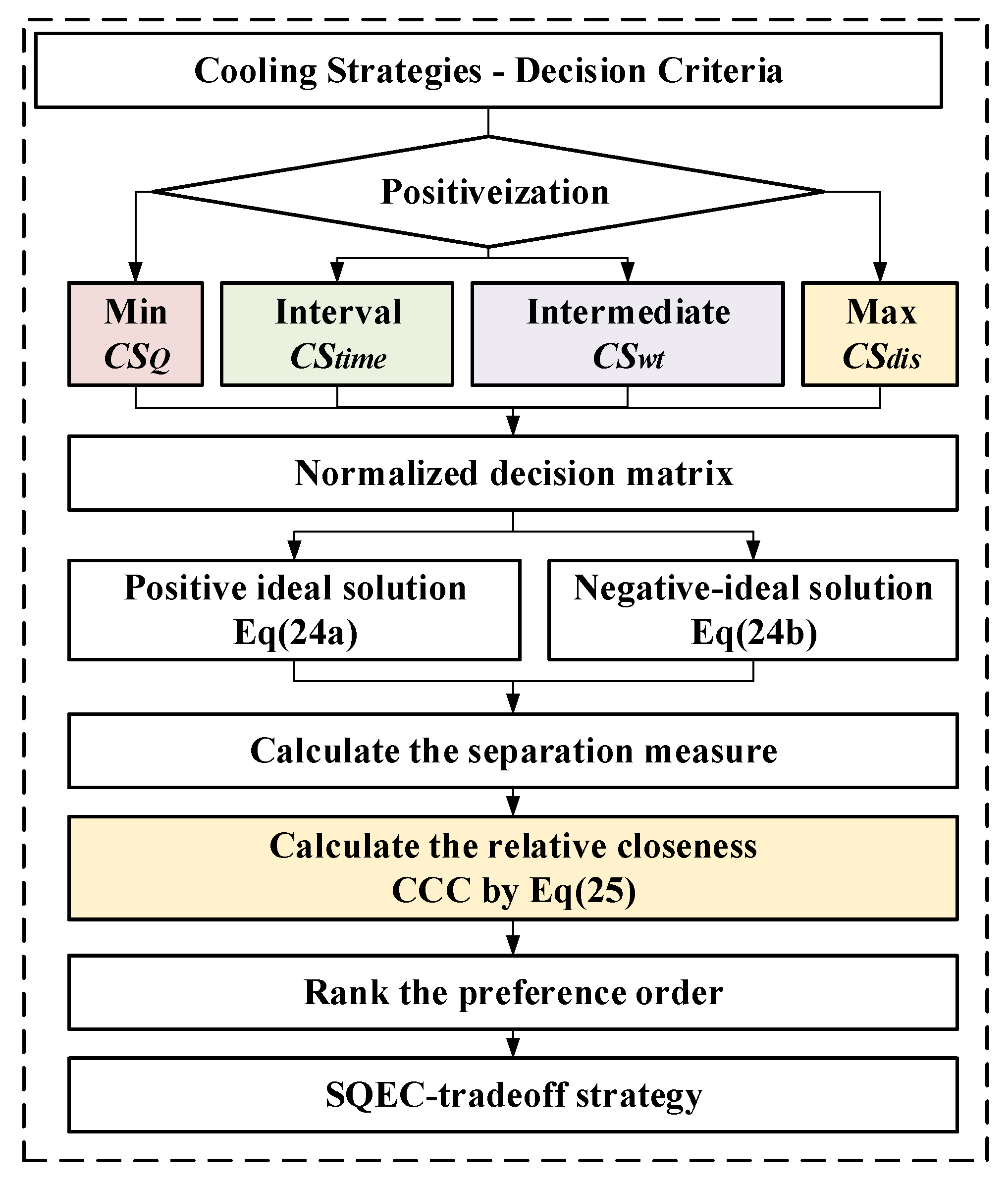
• In practical engineering projects, water pipe spacing is considered a maximum indicator, where increased spacing leads to lower costs due to reduced expenses on materials, labor, and space. This is especially significant in dam construction, where the costs of transporting, storing, and placing water pipes on the dam are extensive.
• Cooling water flow rate is viewed as a minimum indicator, with smaller flow rates providing greater benefits. High-powered pumps are required to achieve high-flow cooling water, generating additional energy consumption, particularly during the construction of dams, where limited space and height differences in the water system require specialized design considerations.
• Cooling water temperature is regarded as an intermediate-type indicator due to its effect on the temperature gradient around the cooling water pipe. If the water temperature is too low, it can result in a large temperature gradient, which increases the risk of cracking around the water pipe [7]. Conversely, high water temperature in the cooling water pipe affects cooling efficiency, and controlling cooling water temperature often requires high power compressors. Compressors are energy-intensive devices that incur high cooling costs, particularly when the external ambient temperature is significantly higher than the target temperature.
• Cooling time is classified as an interval-type indicator. Prolonged cooling times can lead to increased costs, while too-short cooling times can result in incomplete hydration heat release of concrete, leading to temperature recovery issues later on [54], which ultimately has a detrimental effect on the structure. Typically, around 60–80% of the heat of hydration is released after around 28 days of concrete age, with more than 90% released when the design age of 90 days is reached. Therefore, cooling time needs to correspond with the design strength attainment of the concrete material, with the cooling time being determined by a surrogate model.

Therefore, a multi-criteria decision model using TOPSIS is constructed based on the Pareto optimal solution set of NSGA2 multi-objective optimization and the cost-effective response mechanism of the cooling system to obtain an optimal strategy for ensuring safety, quality, efficiency, and cost balance.

3. Implementation of SQEC-TSOM

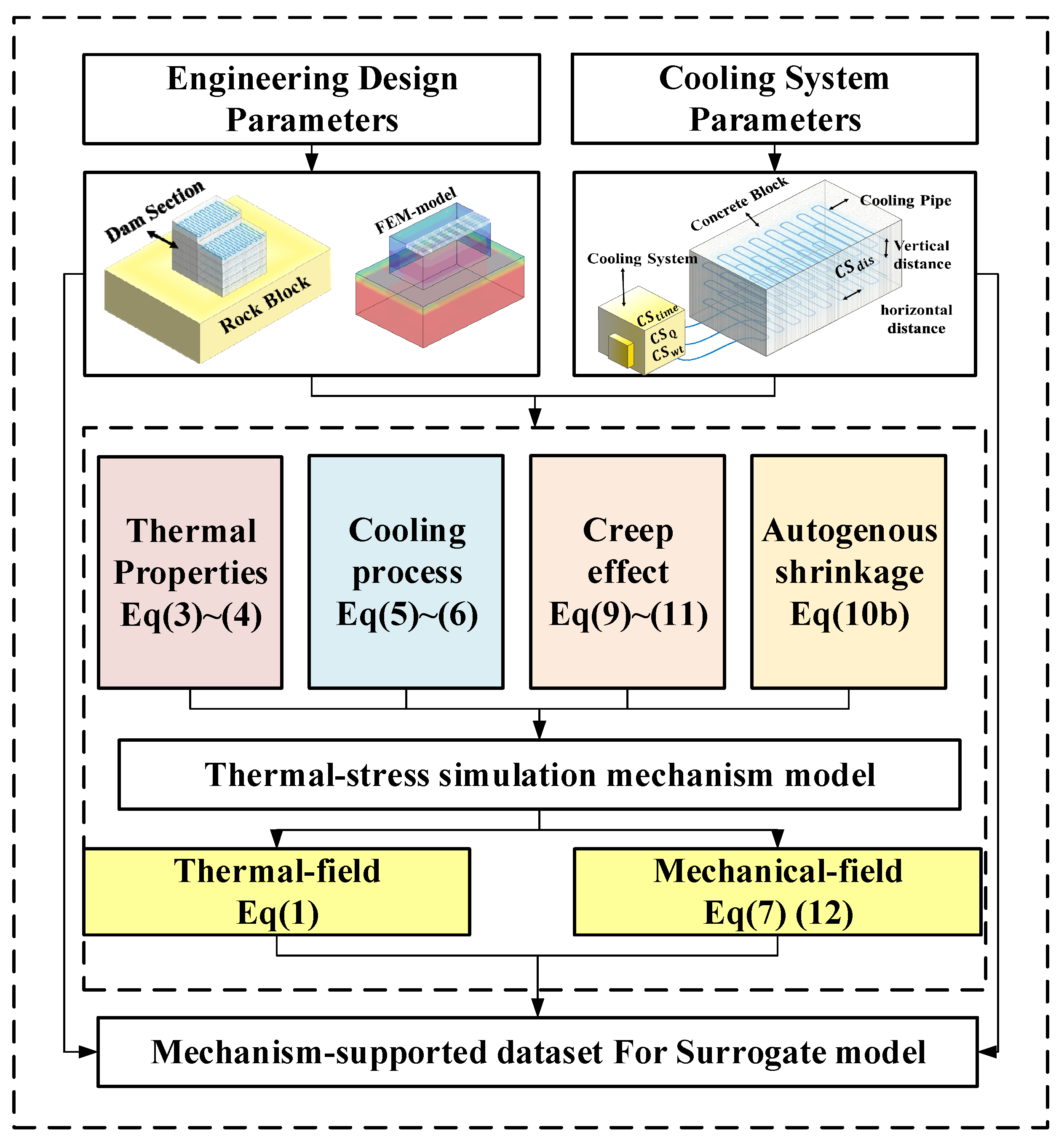
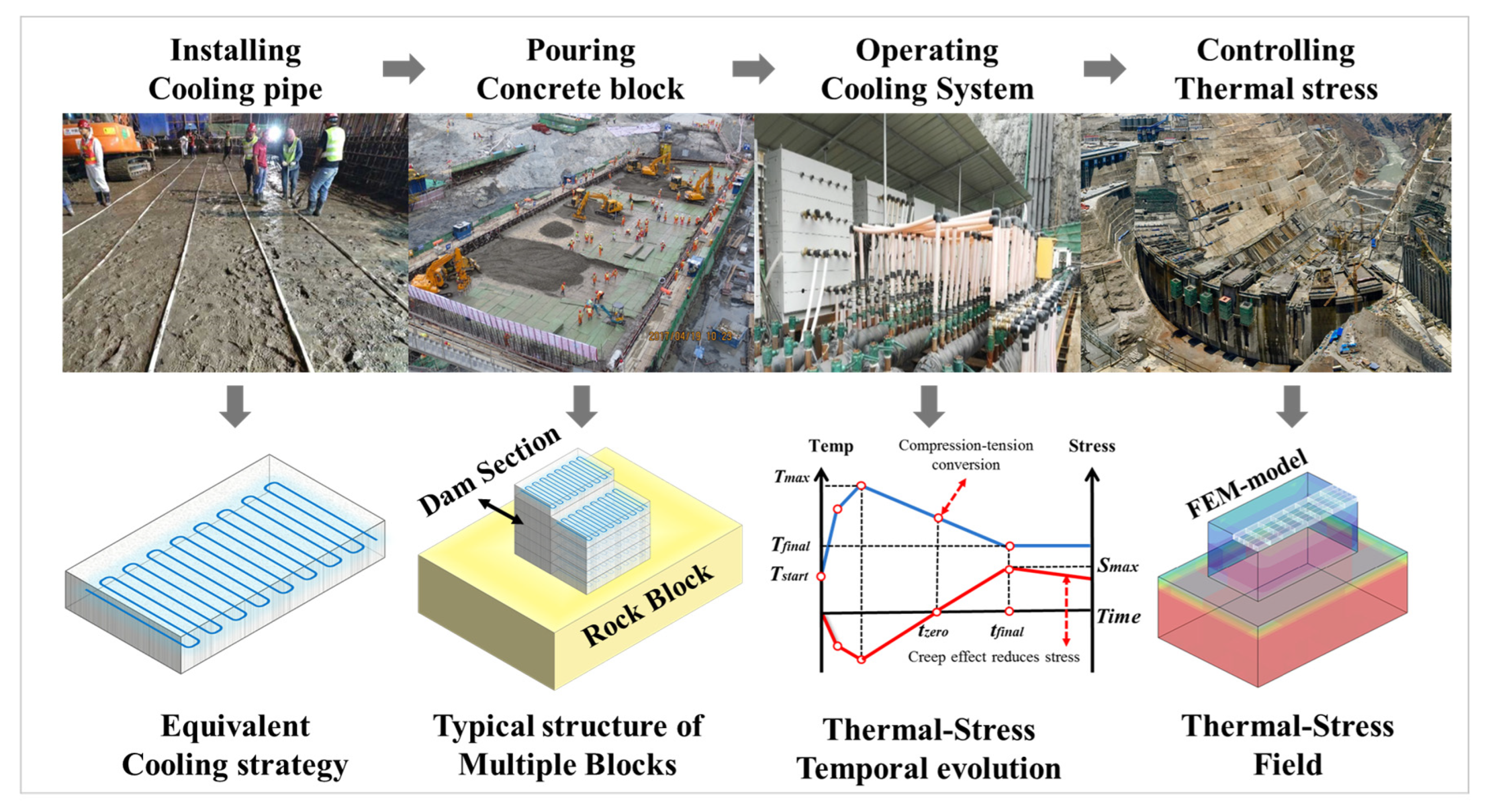
3.1. Implementation of TSMM

The full-process Thermal Stress Simulation Mechanism Model (TSMM) enables the comprehensive simulation of the structure, from casting to temperature stabilization, through coupled thermodynamic calculations. It evaluates safety based on failure criteria, as illustrated in Figure 2.

Accurate evaluation of temperature and stress response under different cooling strategies requires considering the design parameters of the engineered structure (including structural properties, material properties, construction properties, and boundary conditions), as well as the cooling system parameters. The key to the multi-field coupling analysis lies in the temperature and mechanical fields, where heat transfer, heat of hydration in concrete, and cooling characteristics of water pipes are the primary considerations in the temperature field. In the mechanical field, the analysis takes into account the effects of gravity, temperature, and creep characteristics on the structure. Safety assessment considers concrete strength and stress development levels. The full process safety factor is calculated based on the maximum stress failure criterion. Additionally, the strength assessment incorporates the influence of temperature and humidity on the equivalent age for a more accurate safety assessment.

The construction aspect primarily involves sequencing unit casting during the construction process. To facilitate this, an automated simulation calculation and post-processing program was developed using MSC Marc2012 software and Python. This program automatically calculates and generates temporal–spatial stress and temperatures based on cooling strategies, providing an essential dataset support for the surrogate model.

3.1.1. Temperature Field Simulations

Heat Conduction

According to the heat transfer theory, the descriptive equations and boundary conditions of the unsteady temperature field of concrete structures can be expressed as follows [1]:

$${\displaystyle \frac{\partial T}{\partial \tau }}=a\left({\displaystyle \frac{{\partial }^{2}T}{\partial x^2}}+{\displaystyle \frac{{\partial }^{2}T}{\partial y^2}}+{\displaystyle \frac{{\partial }^{2}T}{\partial z^2}}\right)+{\displaystyle \frac{\dot{Q}}{\rho \mathrm{c}}}$$

(1a)

$$\begin{gathered} \mathrm{Dirichlet} \mathrm{boundary} \mathrm{condition}: \\ {T}_{\mathrm{s}}\left(\tau \right)=f_1\left(\tau \right) \end{gathered}$$

(1b)

$$\begin{gathered} \mathrm{Neumann} \mathrm{boundary} \mathrm{condition}: \\ -\lambda {\displaystyle \frac{\partial T}{\partial n}}=f_2\left(\tau \right) \end{gathered}$$

(1c)

$$\begin{gathered} \mathrm{Robin} \mathrm{boundary} \mathrm{condition}: \\ -\lambda {\displaystyle \frac{\partial T}{\partial n}}=\beta \left(T_{\mathrm{s}}-T_{\mathrm{a}}\right) \end{gathered}$$

(1d)

where $a$ is thermal conductivity coefficient; $\mathrm{c}$ is specific heat capacity; $\rho$ is density; $\lambda$ is thermal conductivity; $\dot{Q}$ is the heat emitted per unit volume per unit time; $T_{\mathrm{s}}$ is the surface temperature; $\tau$ is time; $f_1$ is a known function that varies with time; $\beta$ is the surface heat dissipation coefficient; $T_{\mathrm{a}}$ is air temperature; and $n$ is the outward normal direction. When the adiabatic condition is met, ${\displaystyle \frac{\partial T}{\partial n}}=0$.

The temperature change in concrete is mainly determined by both the exothermic hydration and the cooling system, so the heat change per unit volume of concrete can be expressed as follows:

$$\dot{Q}\left(\tau \right)={\dot{Q}}^{-}\left(\tau \right)+{\dot{Q}}^{+}\left(\tau \right)$$

(2)

where ${\dot{Q}}^{-}$ denotes the cold source intensity of the cooling water pipe, and ${\dot{Q}}^{+}$ denotes the heat source intensity of the exothermic hydration.

Thermal Properties of Materials

$${\dot{Q}}^{+}\left(\tau \right)=c\rho {\theta }_{\left(\tau +\Delta \tau /2\right)}^{\prime }$$

(3)

$$\theta ={\theta }_{0}s\left(1-{\mathrm{e}}^{-m_1\tau }\right)+{\theta }_0\left(1-s\right)\left(1-{\mathrm{e}}^{-m_2\tau }\right)$$

(4)

where $\theta$ is the heat of hydration function, indicating the adiabatic temperature rise of concrete at $\tau$ days in °C; ${\theta }_0$ is the final adiabatic temperature rise; $\tau$ indicates the age of concrete; and $m_1$, $m_2$, and $s$ are the fitted parameters. This formula has the advantages of being mathematically convenient for calculations and showing good agreement with experimental data.

The adiabatic temperature rise of the material is one of the significant factors influencing temperature-control strategies, related to the physicochemical characteristics of material components and mix proportions. The provided framework for mechanistic analysis and the process is fixed, but the material performance model is not constrained by the framework, which is an important consideration when applying the model. For the dam concrete studied in this article, Formula (4) is used to calculate the values satisfying the project requirements based on the results of adiabatic temperature rise tests. Details of the specific parameters can be found in Section 4.1.2, “Calculation Parameters Configuration”.

Cooling System Simulation

The heat exchange between water pipes and concrete results in changes in water temperature within the pipe. Approaches to managing the water temperature along the pipe can be categorized into decoupled and coupled methods. The decoupled method separates the concrete and water pipe temperatures, treating the current step water temperature as a boundary condition to establish a finite element equation for the concrete temperature and subsequently deducing the distribution of water temperature along the pipe for the next step. Since water and concrete temperatures cannot be solved simultaneously, the decoupled approach generally requires iterative calculations to obtain more accurate results. The coupled method, on the other hand, considers both water and concrete temperatures as degrees of freedom and solves them simultaneously within the finite element equation. Both methods necessitate refined meshes, resulting in large computational scales and extremely low efficiency, which do not meet the demands of dam engineering projects. Therefore, this employs an equivalent simulation method for cooling.

$${\dot{Q}}^{-}\left(\tau \right)=c\rho \left[T\left(\tau \right)-T_w\right]{\varphi }_{\left(\tau +\Delta \tau /2\right)}^{\prime }$$

(5)

where $\varphi$ is the cooling effect function, $T_w$ is the cooling water temperature, and $\Delta \tau$ is the incremental step.

$$\varphi \left(t\right)=\exp \left(-k_1{z}^s\right)$$

(6a)

where

$$\begin{gathered} k_1=2.08-1.174\xi +0.256{\xi }^2 \\ s=0.971+0.1485\xi -0.0445{\xi }^2 \\ z={\displaystyle \frac{gat}{D^2}} \end{gathered}$$

(6b)

$$\xi ={\displaystyle \frac{\lambda L}{c_w{\rho }_w{q}_w}}$$

(6c)

$$D_c=1.1672\sqrt{D_1{D}_2}$$

(6d)

where $k_1$ and $s$ are fitting coefficients, which are related to the thermal properties of concrete, the length of the water pipe, and the flow rate through the water; $s$ is the thermal conductivity of concrete; $L$ is the length of the cooling water pipe; $c_w$, ${\rho }_w$, and $q_w$ are the specific heat, density, and flow rate of water, respectively; $g$ is the ratio of the equivalent thermal conductivity coefficient to the thermal conductivity coefficient, $a$, which is used to consider the radius of the cooling water pipe and the influence of the material [1]; $D_c$ is the equivalent cooling diameter, which is related to the cooling water tube spacing; $D_1$ is the vertical spacing; and $D_2$ is the horizontal spacing.

In the equivalent simulation, the computational length, L, of the cooling water pipe is set at 220 m, aligned with practical engineering circumstances where the cooling water pipe length is 220 m. The cooling system uses a direction-changing device to modify the flow, which effectively controls the temperature difference between the water inlet and outlet within 2 °C. Consequently, the equivalent simulation method can be used to accurately simulate the effects of the cooling water pipes.

Therefore, the above equation takes into account the parameters affecting the cooling effect, including the cooling water pipe spacing, cooling water temperature, cooling flow rate, and water passage time, and therefore can be used for the evaluation of the cooling strategy.

3.1.2. Stress Field Simulation

The finite element method is used to analyze the deformation and stresses in concrete structures. Since the effect of creep has a great influence on the stress level of mass concrete, and some studies have shown that the stress relaxation at an early age can reach 50% or even more, creep is taken into account in the analysis process [12].

Since the structural safety assessment requires obtaining the stress levels for the whole process, each time step needs to be analyzed, and the following is an example of the deformation and stress calculation method for a certain time step, $n$:

$$\left\{\Delta {\epsilon }_n\right\}=\left\{\Delta {\epsilon }_n^{\mathrm{e}}\right\}+\left\{\Delta {\epsilon }_n^{\mathrm{c}}\right\}+\left\{\Delta {\epsilon }_n^{\mathrm{T}}\right\}+\left\{\Delta {\epsilon }_n^{\mathrm{ch}}\right\}$$

(7)

where $\Delta {\epsilon }_n^{\mathrm{e}}$ is the elastic strain increment, $\Delta {\epsilon }_n^{\mathrm{c}}$ is the creep strain increment, and $\Delta {\epsilon }_n^{\mathrm{T}}$ is the temperature strain increment.

$$\left\{\Delta {\epsilon }_n^{\mathrm{e}}\right\}={\displaystyle \frac{1}{E\left({\overline{\tau }}_n\right)}} \left[Q\right]\left\{\Delta {\sigma }_n\right\}$$

(8a)

$$E\left(\tau \right)=E_0\left(1-{\mathrm{e}}^{-a{\tau }^b}\right)$$

(8b)

$${\overline{\tau }}_n=\left({\tau }_{n-1}+{\tau }_n\right)/2$$

(8c)

where $E\left({\overline{\tau }}_n\right)$ is the current time-step equivalent elastic modulus; $\left[Q\right]$ is the coefficient matrix; $\Delta {\sigma }_n$ is the current step stress increment; $E_0$ is the final elastic modulus; and $a$ and $b$ are the material-dependent constants.

$$\left\{\Delta {\epsilon }_n^{\mathrm{c}}\right\}=\left\{{\eta }_n\right\}+C\left(t,{\overline{\tau }}_n\right) \left[Q\right]\left\{\Delta {\sigma }_n\right\}$$

(9a)

$$\left\{{\eta }_n\right\}={\displaystyle \sum }_s\left(1-{\mathrm{e}}^{-r_s\Delta {\tau }_n}\right)\left\{{\omega }_{sn}\right\}$$

(9b)

$$\left\{{\omega }_{sn}\right\}=\left\{{\omega }_{s,n-1}\right\}{\mathrm{e}}^{-r_s\Delta {\tau }_{n-1}}+\left[Q\right]\left\{\Delta {\sigma }_{n-1}\right\}{\mathsf{\Psi }}_s\left({\overline{\tau }}_{n-1}\right){\mathrm{e}}^{-0.5r_s\Delta {\tau }_{n-1}}$$

(9c)

$$C\left(t,\tau \right)={\displaystyle \sum }_{s=1}^m{\mathsf{\Psi }}_s\left(\tau \right)\left[1-{\mathrm{e}}^{-r_s\left(t-\tau \right)}\right]$$

(9d)

$$\begin{array}{l}{\mathsf{\Psi }}_s\left(\tau \right)=f_s+g_s{\tau }^{-p}, \mathrm{when} s=1 \mathrm{to} m-1\\ {\mathsf{\Psi }}_s\left(\tau \right)=D{\mathrm{e}}^{-r_s\tau }, \mathrm{when} s=m\end{array}\}$$

(9e)

where $C\left(t,\tau \right)$ is the creep produced under unit stress; $\tau$ denotes the loading time; and $f_s$, $g_s$, $r_s$, and $D$ are all the creep parameters determined by the test. Equation (9b) integrates the aging theory, and elasticity creep theory can better describe the early age and long-term creep of concrete. In this paper, s is taken as 3, and the accuracy is sufficient for engineering calculations.

Using the B4 model to account for autogenous shrinkage, it is transformed into an incremental form, as shown in Equation (10b) [25]:

$$\left\{\Delta {\epsilon }_n^{\mathrm{T}}\right\}={\left[\alpha \Delta T_n,\alpha \Delta T_n,\alpha \Delta T_n,0,0,0\right]}^{\mathrm{T}}$$

(10a)

$$\left\{\Delta {\epsilon }_n^{\mathrm{ch}}\right\}={\left[\chi \Delta {\xi }_n,\chi \Delta {\xi }_n,\chi \Delta {\xi }_n,0,0,0\right]}^{\mathrm{T}}$$

(10b)

where $\alpha$ is the linear expansion coefficient, $\Delta T_n$ is the temperature increment at step $n, \chi$ is the shrinkage coefficient, and ${\xi }_n$ is the autogenous shrinkage increment at step $n$.

$$\left\{\Delta {\sigma }_n\right\}=\left[{\overline{D}}_n\right]\left(\left\{\Delta {\epsilon }_n\right\}-\left\{{\eta }_n\right\}-\left\{\Delta {\epsilon }_n^{\mathrm{T}}\right\}-\left\{\Delta {\epsilon }_n^{\mathrm{ch}}\right\}\right)$$

(11a)

$$\left[{\overline{D}}_n\right]={\overline{E}}_n {[Q]}^{-1}$$

(11b)

$${\overline{E}}_n={\displaystyle \frac{E\left({\overline{\tau }}_n\right)}{1+E\left({\overline{\tau }}_n\right)C\left(t_n,{\overline{\tau }}_n\right)}}$$

(11c)

where ${\overline{D}}_n$ is the equivalent elastic matrix.

Therefore, the stress level of an element at step $n$ can be expressed as

$$\left\{{\sigma }_n\right\}=\left\{\Delta {\sigma }_1\right\}+\left\{\Delta {\sigma }_2\right\}+\cdots +\left\{\Delta {\sigma }_n\right\}=\sum \left\{\Delta {\sigma }_n\right\}$$

(12)

3.1.3. Safety Performance Assessment

Massive concrete damage is usually caused by excessive tensile stresses, so the maximum tensile stress damage criterion is used to calculate the safety factor, which can be expressed as follows:

$$K_n={\displaystyle \frac{{\tau }_n}{{\sigma }_n}}$$

(13a)

$${\tau }_n=f_{t,90}\left(1-{\mathrm{e}}^{{a{t}_e}^b}\right)$$

(13b)

$$t_e={\displaystyle \sum }_i^{n-1}{\displaystyle \frac{1}{{\alpha }_u-{\alpha }_0}}{\left({\displaystyle \frac{T_i}{T}}\right)}^{-m}exp\left[-{\displaystyle \frac{E_a}{R}}\left({\displaystyle \frac{1}{T_i}}-{\displaystyle \frac{1}{T}}\right)\right]\left[H_i\cdot \Delta t_i+{\displaystyle \frac{1-H_i}{\gamma }}ln\left(1+\gamma \cdot t_i\right)\right]$$

(13c)

where ${\tau }_n$ is the concrete splitting strength; ${\sigma }_n$ is the structural stress level; $K_n$ is the safety factor for the nth day of concrete since placement; and $f_{t,90}$ is the design tensile strength of concrete, which is usually 28 d strength for general concrete structures, but for dam concrete, the design strength is usually 90 d or 180 d to reach the design target [55]. This is due to the fact that high early strength means that the hydration rate is fast and the temperature is difficult to control. At the same time, high early strength leads to higher stress levels, which are not conducive to preventing cracking. Furthermore, $a$ and $b$ are constants related to material properties, and $t_e$ is the equivalent age. Since concrete components, curing temperature, and humidity significantly affect performance [56], it is important to take into account material hydration properties, temperature variations, and humidity processes when assessing safety. Moreover, ${\alpha }_u$ is the final degree of hydration; ${\alpha }_0$ is the initial degree of hydration at which the concrete hardens; and for dam concrete, the initial degree of hydration is 0.02. For water–cement ratios between 0.4 and 0.5, the final degree of hydration is 60–70%. $T$ is the standard curing temperature; $T_i$ is the current time-step average temperature; R is the ideal gas constant, equal to 8.314 J/(mol∙K); $E_a$ is the apparent activation energy of concrete, which characterizes the dependence of the chemical reaction rate on temperature; $H_i$ is the current time-step average curing humidity; and γ is the moisture diffusion coefficient, which is related to the fly ash content, water–cement ratio, and other factors [57]. Since mass concrete usually has a high water–cement ratio and the internal humidity is not affected by the external under well-cured conditions, the curing humidity is taken as 100% in this study.

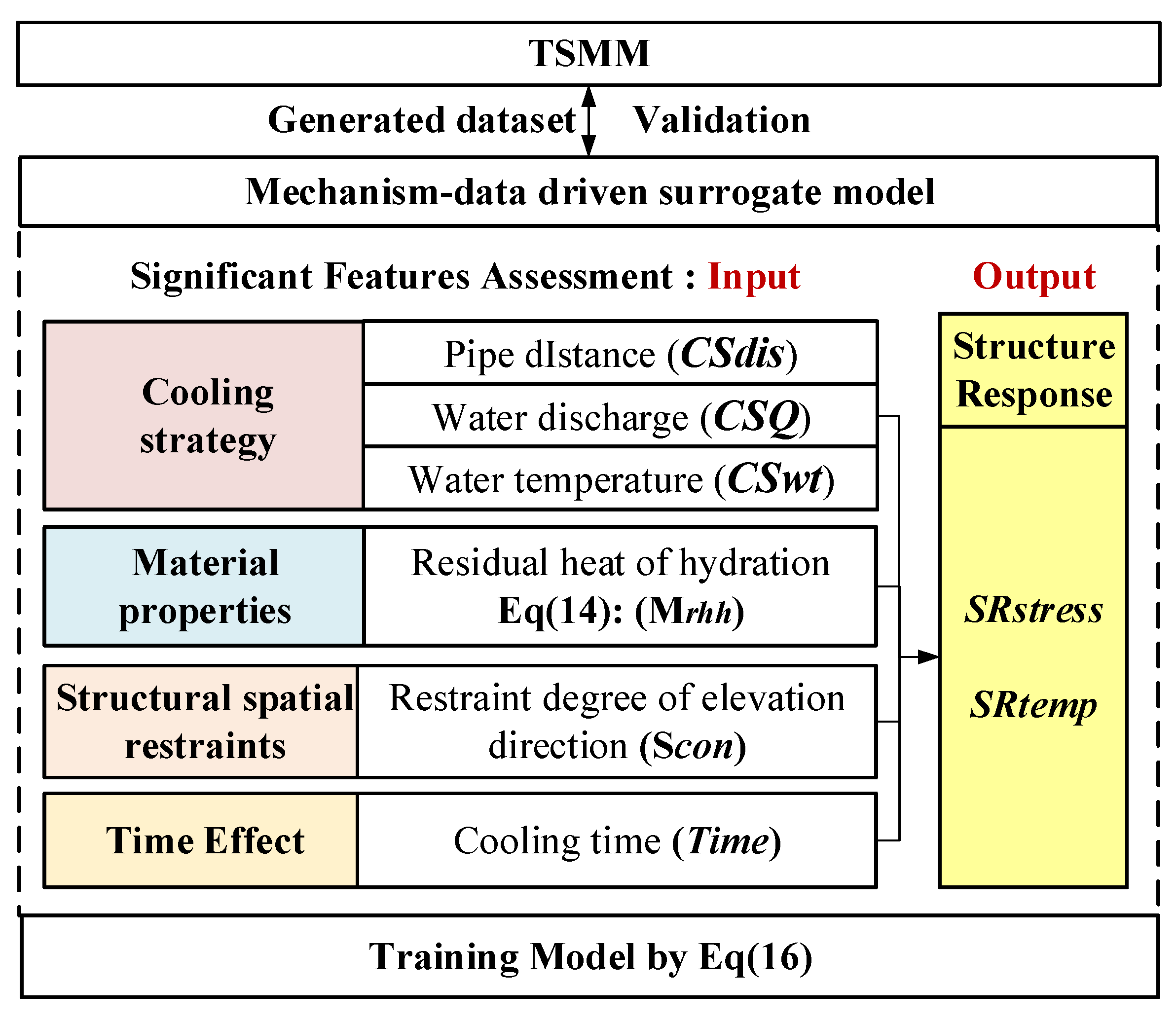
3.2. Implementation of MD-SM

The goal of the surrogate model is to establish the relationship between key factors and the spatiotemporal response of the structure, and to accurately and quickly evaluate the effects of different cooling strategies on structural stresses. Proper features, suitable algorithms, and high-quality datasets are essential to ensure model accuracy and interpretability and improve training efficiency.

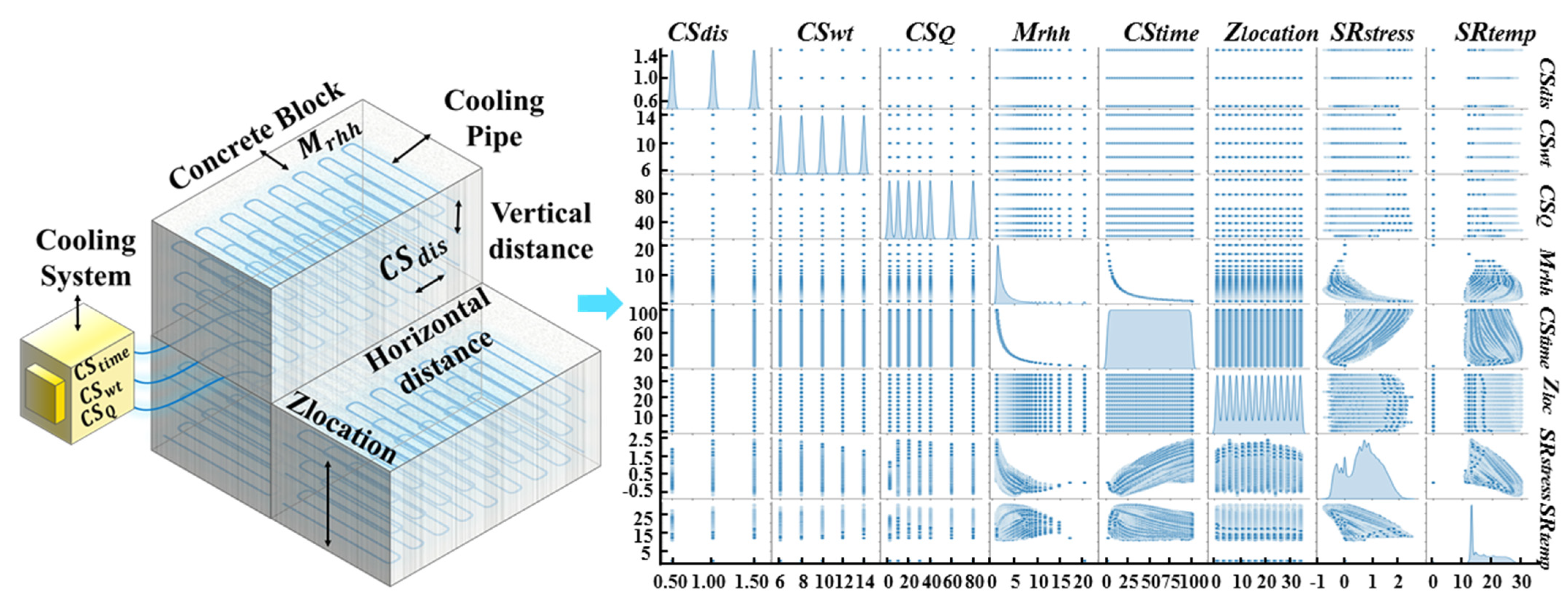
3.2.1. Selection of Important Features

The selection of input and output features for the surrogate model is based on the temporal and spatial evolution of mass concrete temperature and stress. Specifically, important features are chosen as inputs from four aspects: cooling strategies, material properties, structural spatial restraints, and temporal effects. The temperature and stress response of the structure serve as the model’s output (see Figure 3). Here are the details:

From a temperature perspective, the evolution is divided into cooling and exothermic phases. The cooling system, as discussed in Section 3.1, plays a central role in regulating temperature and, consequently, stress levels. The cooling strategy encompasses parameters such as the spacing of cooling water pipes (CSdis), water temperature (CSwt), and water flow rate (CSQ). It should be noted that cooling water pipes are typically made of plastic hose, which possesses relatively fixed thermal properties and is not considered part of the cooling strategy. To facilitate construction, the spacing of cooling water pipes is uniformly arranged in both horizontal and vertical directions. In the case of dams, where casting blocks are typically 3.0 m or 4.5 m in height, the spacing range of pipes from 0.5 m to 1.5 m. The cooling water temperature is determined by the stable external ambient temperature, concrete temperature, and cooling unit capacity. The flow rate of cooling water is usually dependent on the performance of the cooling water pump and the desired cooling efficiency. Research indicates that the flow rate of cooling water pipes is proportional to the cooling efficiency. Given the extensive cooling area of concrete, a longer cooling water pipe exhibits limited cooling effectiveness at lower flow rates (in the laminar flow state), while higher flow rates (in the turbulent flow state) result in improved cooling. Hence, it is crucial to ensure that the flow rate of cooling water is not excessively low.

When boundary conditions remain stable, the heat of hydration of the concrete material serves as the sole heat source, directly influencing the effectiveness of the cooling strategy. Therefore, the residual heat of hydration is utilized as a characteristic to evaluate the material’s exothermic potential. This characteristic can be expressed as follows:

$$M_{rhh}={\theta }_0 \left[1-s\left(1-{\mathrm{e}}^{-m_{1}t}\right)-{\theta }_0\left(1-s\right)\left(1-{\mathrm{e}}^{-m_{2}t}\right)\right]$$

(14)

where $M_{rhh}$ is the residual heat of hydration of the material, and other parameters are detailed in Equation (4).

The evolution of stresses exhibits significant variations both in time and space. Firstly, in terms of time, compressive stresses are generated by the thermal expansion of concrete during the hydration process following pouring. These compressive stresses peak when the maximum temperature ($T_{max}$) is reached. As the cooling system operates, the concrete gradually cools from the maximum temperature, causing the compressive stress to decrease gradually until it reaches zero. Subsequently, as the temperature continues to decrease, tensile stresses increase, reaching their highest level when the temperature stabilizes at the final temperature ($T_{final}$). After this point, the tensile stresses gradually diminish due to the creep effect of the concrete until they stabilize. The entire cooling process typically extends beyond 90 days, necessitating the consideration of time effects.

Secondly, in terms of space, a significant restraint arises due to the substantial difference between the elastic modulus of mass concrete and the underlying foundation rock. This restraint is commonly expressed as the degree of restraint, as described by Xin et al. [14]. Zhu et al. also noted that the degree of restraint for concrete structures constructed on hard rock decreases with increasing elevation [1]. In this study, the elevation (Zlocation) serves as the characterization index for the degree of restraint. By utilizing elevation, the need for complex integral calculations of the confinement degree is circumvented, while enabling the direct determination of stress variations along the vertical direction. This approach provides an opportunity for comprehensive stress assessment across the entire domain.

The surrogate model utilizes the temperature and stress in the central region as input parameters, considering the spatial and temporal response characteristics of temperature and stress in the massive concrete structure. This choice is motivated by the fact that the highest temperature is typically observed at the center of each casting block. When cooling reaches the target temperature, the maximum total temperature gradient and stress level are found at the central location. Consequently, selecting the central region enables the evaluation of the area with the highest risk of cracking while reducing the number of data required for training the surrogate model. This reduction in data is crucial for enhancing the model’s accuracy and efficiency. Therefore, the surrogate model can be mathematically expressed as follows:

$$\sigma =f_{xgb1}\left(C{S}_{dis},C{S}_{wt},C{S}_Q,M_{rhh},S_{rd},Time\right)$$

(15a)

$$T=f_{xgb2}\left(C{S}_{dis},C{S}_{wt},C{S}_Q,M_{rhh},S_{rd},Time\right)$$

(15b)

where $\sigma$ is the stress in the casting block at a certain elevation at a certain time step, and $T$ is expressed as the temperature of the casting block at a certain elevation at a certain time step.

3.2.2. Surrogate Model Selection and Training

Surrogate models offer efficient and accurate approximations compared to mechanistic models. They possess several advantages, including computational efficiency, data efficiency, flexibility, and interpretability. Moreover, surrogate models require fewer computational resources and data compared to finite element models (FEMs), making them widely employed for optimization, sensitivity analysis, and uncertainty quantification. Currently, the commonly used surrogate models comprise statistical models (e.g., response surface models and Gaussian process regression models) and machine learning models (e.g., neural networks, support vector machines, decision trees, and random forests). In handling complex datasets, machine learning models are favored, as they better capture nonlinear relationships between input and output variables, yielding higher accuracy.

Notably, ensemble learning models based on the Boosting framework exhibit higher accuracy and better robustness in classification, regression, and clustering problems. They effectively mitigate the issues of underfitting and overfitting [48]. Furthermore, ensemble learning models surpass individual models, yielding superior results [58,59,60,61].

Therefore, in this study, the XGBoost algorithm is selected to train the surrogate model. XGBoost [48], proposed by Chen et al. in 2016, is an optimized gradient boosting algorithm. It incorporates regularization techniques and parallel processing to enhance prediction accuracy and efficiency, making it suitable for large datasets. XGBoost has been widely applied in diverse domains, showcasing its effectiveness. In the field of concrete, XGBoost has been utilized for predicting concrete stress and resistivity performance, as well as stress evaluation [62,63]. The underlying principle of the XGBoost model is as follows:

$$Obj={\displaystyle \sum }_{i=1}^{n}l\left(y_i,{\widehat{y}}_i\right)+{\displaystyle \sum }_{k=1}^K\mathsf{\Omega }\left(f_k\right)$$

(16)

The XGBoost model utilizes a loss function $l\left(y_i,{\widehat{y}}_i\right)$ and a regularization term, $\mathsf{\Omega }$, as illustrated in Formula (16). This model incrementally adds weak classifiers to continuously improve performance. During each iteration, XGBoost generates a new classifier based on the residual from the previous round and applies this to update model parameters. Additionally, XGBoost implements regularization to prevent overfitting and incorporates second-order gradient information to enhance accuracy. The XGBoost model generates final prediction results through weighted averaging of multiple weak classifiers.

In summary, the XGBoost algorithm is selected as the training algorithm, using mechanisms such as model sensitivity analysis to screen and evaluate critical input characteristics, including structural stress, temperature, and deformation. These selected mechanisms also include material hydration characteristics, cooling strategies, and differences in spatial and temporal dimensions of the structure. The method effectively omits nonessential features, reduces input feature dimensions, increases training efficiency, and improves prediction accuracy.

3.2.3. Assessment of Surrogate Models

The accuracy, efficiency, and interpretability of surrogate models are crucial for ensuring structural safety. As such, this paper evaluates the reliability of the surrogate model through model evaluation indicators and interpretability methods, followed by verifying the surrogate model through a mechanism model.

Regarding model evaluation, we implement the root-mean-square error (RMSE) and coefficient of determination (R²) to assess the surrogate model’s accuracy for regression problems. MSE represents the average square difference between predicted values and actual values. Meanwhile, RMSE represents the square root of MSE and measures the average distance between predicted values and actual values. As for R², it represents the degree of fit between the model and the data. It provides an indication of the proportion of the variance in the dependent variable relative to the independent variables.

$$\mathrm{RMSE} =\sqrt{{\displaystyle \frac{1}{m}}{\displaystyle \sum }_{i=1}^m{\left(y_i-{\widehat{y}}_i\right)}^2}$$

(17a)

$$R^2=1-{\displaystyle \frac{{{\displaystyle \sum }}_i{\left({\widehat{y}}_i-y_i\right)}^2}{{{\displaystyle \sum }}_i{\left({\overline{y}}_i-y_i\right)}^2}}$$

(17b)

where ${\widehat{y}}_i$ is the predicted value, and $y_i$ is the true value.

In terms of interpretability, the study utilizes feature importance analysis and SHAP value analysis methods. Feature importance evaluates the significance of each feature in the model by calculating the number of splits or the impact of splits (i.e., information gain) associated with each feature. Typically, features are ranked in descending order based on their importance, allowing the identification of the most influential ones for predicting the target variable. In 2017, Lundberg and Lee introduced SHAP values, a local explanation method that decomposes the model’s predicted value into contributions from each feature, with the sum of these contributions representing the predicted value [64]. SHAP values quantify the extent of influence that each feature has on the model’s predicted value. Wu et al. employed the Shapley additive explanation method to assess factors influencing concrete strength [58]. Compared to feature importance, SHAP values offer more accurate and detailed information, thereby facilitating a better understanding of the model’s decision process and the interplay between features. Through a comprehensive evaluation that compares the rankings obtained from both methods with the sensitivity analysis results of mechanistic models, the interpretability of the model is thoroughly examined.

3.2.4. Datasets and Model Training

The accuracy of the model heavily relies on the quality and quantity of data. Therefore, it is crucial to generate a high-quality dataset using the mechanistic model. Therefore, cooling strategies are generated based on the range of cooling system performance parameters in engineering (including the performance of cooling units, controllability of pumps, water pipe spacing, etc.), and orthogonalized and training datasets are constructed through TSSM model calculations.

For dataset generation and model training, the following three aspects should be considered: First, the performance of the cooling system should be thoroughly examined, and strategy combinations should be generated to cover all possible limit states, providing a feasible solution space for the optimization model. Second, the dataset should be expanded based on the loss function and model prediction metrics on the training and test sets, aiming to enhance the model’s accuracy and generalization performance. Third, the parameters and hyperparameters of the agent model should be optimized to improve the efficiency and prediction accuracy during training. Last, the accuracy and generalization performance of the model are evaluated using the mechanistic model, and the agent model that satisfies both mechanism-driven and data-driven approaches is retained.

3.3. Implementation of IOM

The objective of the multi-objective optimization model based on NSGA2 is to obtain the Pareto solution set, which represents a set of non-inferior optimal solutions that achieve a balance between safety, quality, and efficiency. Hence, the key to solving the multi-objective optimization problem lies in finding the Pareto solution set based on the objective function and constraints, as depicted in Figure 4.

3.3.1. Objective Function

(1) Material quality evaluation function (QEF)

The QEF quantifies the efficiency of material quality utilization by measuring the proximity of the safety factor of the entire process for all units to the design safety factor. A smaller QEF value is indicative of higher material performance. Mathematically, QEF can be expressed as follows:

$$\min \mathrm{QEF}(C{S}_{dis},C{S}_{wt},C{S}_Q)=\sqrt{{\displaystyle \frac{1}{mn}}{\displaystyle \sum }_{i=1}^m{\displaystyle \sum }_{j=1}^n{\displaystyle \frac{{\left(k_{ij}-k_i^d\right)}^2}{{\left(k_i^d\right)}^2}}}$$

(18)

where $k_{ij}$ is the safety factor of the cast block at elevation $i$ at age $j$, calculated by Equation (13a), which calls for the surrogate model to predict the stresses; and $k_i^d$ refers to the minimum safety factor required for designing the cast block at elevation $i$. The design factor of safety for dams typically varies due to different degrees of restraint in different parts of the structure. It also serves as the safety reserve of the structure, with the strongly confined area where concrete is closer to bedrock requiring higher safety factors than the unconfined area. Typically, safety factors for dams range from 2.0 to 4.0 [1].

(2) Cooling efficiency evaluation function (EEF)

The overall efficiency of the cooling process is evaluated using the efficiency evaluation function (EEF), which quantifies the time required for all units to reach a stable temperature field. The effectiveness of the cooling process is indicated by a shorter total time, indicating a higher level of efficiency. Mathematically, the EEF can be expressed as follows:

$$\min \mathrm{EEF}(C{S}_{dis},C{S}_{wt},C{S}_Q)={\displaystyle \sum }_{i=1}^m{t}_i^{final}$$

(19)

where $t_i^{final}$ represents the cooling time of the i-th elevation cast block, required to reach the target temperature. The predicted stress is determined using the surrogate model, and the value for $t_i^{final}$ is calculated based on the position at which the stress process curve reaches its maximum value.

As mentioned earlier, due to the difference in boundary conditions, the time to reach the stabilization temperature varies for different casting units under the same cooling strategy. Therefore the time to reach the final temperature of all casting units is to be taken into account in order to achieve the global optimum.

3.3.2. Constraints

The constraints are divided into two types: structural safety constraints and cooling system performance constraints. The strategies that violate the structural safety constraints are excluded based on the maximum tensile stress damage criterion of concrete; the strategy generation range is restricted based on the capacity of the cooling system in the genetic algorithm.

The degree of constraint violation by an individual is judged by the structural safety evaluation function (SEF):

$$SEF(C{S}_{dis},C{S}_{wt},C{S}_Q,M_{rhh},S_{rd},Time)=k_{ij}-k_i^d⩾0$$

(20)

In the calculation process, the constraint violation (CV) matrix is generated by SEF, and the degree of constraint violation is calculated for each individual based on the feasibility law [65]. When SEF < 0, then constraint violation is indicated, and the smaller the value of SEF, the higher the degree of constraint violation, so the constraint matrix parameters are passed in to adjust the fitness when calculating the individual fitness. The purpose of this is to make the solutions that violate the constraints lose their advantage in the genetic selection process so that they are eventually eliminated, which in turn ensures that all feasible solutions meet the security requirements.

The cooling water pipe strategy directly impacts cooling efficiency. A smaller spacing between pipes can enhance cooling performance. However, it may increase construction difficulty and cost. The spacing is typically selected based on structural characteristics and cooling efficiency, often rounded to an integer value for ease of construction control. The temperature of the cooling water is also a crucial factor influencing the cooling system’s performance. Lower water temperatures can provide better cooling efficiency. However, the energy consumption for cooling the feed water is significantly high, particularly under high ambient temperatures. The energy consumption exhibits a nonlinear rapid growth as the temperature decreases. On the other hand, the cooling rate of concrete increases slowly due to its poor thermal conductivity. Consequently, the cooling water temperature is usually determined considering factors such as ambient temperature, target temperature, and cost. The flow rate of the cooling water is another key parameter. Higher flow rates can enhance cooling efficiency. However, they also lead to increased energy consumption and the risk of pipe burst, thereby raising concerns about cracking and maintenance costs. Hence, the cooling strategy should adhere to the following constraints:

$$\{\begin{array}{l}0.5\mathrm{m}⩽C{S}_{dis}⩽1.5\mathrm{m}\\ 6^{\circ }\mathrm{C}⩽C{S}_{wt}⩽{14}^{\circ }\mathrm{C}\\ 10{\mathrm{m}}^3/d⩽C{S}_Q⩽80{\mathrm{m}}^3/d\end{array}$$

(21)

3.3.3. Algorithm Process of NSGA2

In order to solve the multi-objective optimization problem mentioned above, the NSGA2 algorithm is used to find the Pareto solution set that satisfies the objective functions and constraints. The NSGA2 algorithm is an improved version of the NSGA algorithm proposed by Kalyanmoy Deb. Compared with other optimization algorithms, NSGA2 not only has the advantages of fast convergence, diversity preservation, strong scalability, high robustness, and low complexity [51], but it also can incorporate prior knowledge of temperature stress control into the constraints and target function. The NSGA2 algorithm uses non-dominated sorting and crowding distance allocation to promote the convergence of optimization strategies to the Pareto front. This mechanism ensures that the algorithm quickly finds the optimal solution and avoids premature convergence. At the same time, NSGA2 maintains the diversity of solution sets by promoting the selection of non-dominated solutions with high crowding distances. This method ensures that the algorithm explores different areas of the search space and prevents convergence to a single solution. Therefore, the NSGA2 algorithm has been widely used in engineering, economics, and other fields, and it has shown excellent performance in solving complex multi-objective optimization problems.

The optimization process of the NSGA2 algorithm is shown in Figure 4 and includes initialization, evaluation, ranking, crowding distance allocation, selection, mutation, and termination. First, the initialization step randomly generates an initial population of candidate solutions. In the evaluation step, the fitness of each candidate solution is evaluated by calculating their objective functions QEF, EEF, and the constraint violation matrix based on SEF, using the surrogate model. The ranking step assigns non-dominated levels to each potential solution. The crowding distance allocation step calculates the crowding distance of each candidate solution based on their neighboring solutions. The selection step selects candidates for the next generation based on their non-dominated levels and crowding distances. The mutation step applies crossover and mutation operators to generate new candidate solutions. The termination step checks the stopping criteria, such as the maximum number of generations or convergence of the objective function value. If the criteria are not met, the algorithm returns to the evaluation step. Otherwise, it returns the Pareto optimal solution set. Based on the NSGA2 optimization model, cooling strategies that satisfy the balance of safety–quality–efficiency can be quickly found.

3.4. Implementation of MCDM

The goal of the multi-criteria decision model is to select the most economical solution from the set of Pareto solutions that satisfy safety–quality–efficiency based on the cooling system design-operating cost characteristics. Firstly, the decision model approach is determined; secondly, the cost–benefit evaluation index is selected; and finally, the optimal strategy is obtained by the decision model.

The selection of decision models suitable for cost–benefit evaluation is crucial. Multi-criteria optimization methods, including TOSIS (Technique for Order Preference by Similarity to Ideal Solution), AHP (Analytic Hierarchy Process), ELECTRE (Elimination and Choice Translating Reality), EDA (Elimination and Choice Expressing Reality), RSR (Rank Sum Ratio), and others are widely used in engineering. Compared with other methods, TOPSIS evaluates cost and benefits more comprehensively since it considers both the best and worst solution strategies. Additionally, TOPSIS can handle multiple criteria simultaneously, while AHP and EDA methods are primarily used for pairwise comparisons. Furthermore, TOPSIS is a nonparametric method that does not require making assumptions about data distribution, making it highly flexible and applicable. Due to its advantages, TOPSIS and its modified methods are often utilized in cost–benefit assessments. Therefore, in this paper, the TOPSIS method is chosen to construct the decision model, and the optimization process is depicted in Figure 5.

The impact of different elements of the assessment strategy on cost-effectiveness is another important aspect of the multi-criteria assessment. Considering the cooling system design cost, four categories were established to assess cost effectiveness, namely maximum indicator, minimum indicator, interval type indicator, and intermediate type indicator, as shown in

Table 1. Indicator types of the cooling system.

Strategies	Type of Indicator	Characteristics of Indicators
$C{S}_{dis}$	Maximization	Greater spacing between water pipes results in lower costs.
$C{S}_Q$	Minimization	Lower flow rates yield higher benefits.
$C{S}_{time}$	Interval type	The ideal cooling time corresponds to the release of 70% to 90% of the heat of hydration from the concrete.
$C{S}_{wt}$	Intermediate	The ideal water temperature should be maintained at a certain value, both to avoid cracking due to excessive gradients and to avoid temperatures too high to reach the target temperature and thus cost.

.

The process of preferential cost-based strategy is illustrated in Figure 5. Firstly, the indicators of different types are transformed into positive values, forming a decision matrix. Subsequently, the decision matrix is normalized to enable direct comparison among the various indicators. Optimal and inferior indicators are identified based on their respective types, and positive and negative ideal solutions are determined. The distance between each candidate solution and the ideal and negative ideal solutions is then calculated, along with the similarity of each candidate solution to the optimal solution, based on the calculated distances. Finally, the optimal strategy and solution that achieve a balance between safety, quality, efficiency, and cost are obtained by ranking according to the degree of similarity.

Indicator positivization:

$$\begin{gathered} M=max\left\{x_i\right\}, {\tilde{x}}_i=M-x_i \\ M=max\left\{\left|x_i-x_{\mathrm{best} }\right|\right\},{\tilde{x}}_i=1-{\displaystyle \frac{\left|x_i-x_{\mathrm{best} }\right|}{M}} \\ M=max\left\{a-min\left\{x_i\right\},max\left\{x_i\right\}-b\right\},{\tilde{x}}_i=\{\begin{array}{lll}1-{\displaystyle \frac{a-x}{M}}& ,& x<a\\ 1& ,& a\le x\le b\\ 1-{\displaystyle \frac{x-b}{M}}& ,& x>b\end{array} \end{gathered}$$

(22)

Matrix normalization:

$$z_{ij}=x_{ij}/\sqrt{{\displaystyle \sum }_{i=1}^n{x}_{ij}^2}$$

(23)

where $x_{ij}$ denotes the $j$ indicator in the $i$ strategy.

The positive ideal solution (PIS) and negative ideal solution (NIS) are then calculated:

$$\begin{array}{c}{Z}^{+}=\left(Z_1^{+},Z_2^{+},\cdots ,Z_m^{+}\right)\\ =\left(max\left\{z_{11},z_{21},\cdots ,z_{n1}\right\},\cdots ,max\left\{z_{1m},z_{2m},\cdots ,z_{nm}\right\}\right)\end{array}$$

(24a)

$$\begin{array}{c}{Z}^{-}=\left(Z_1^{-},Z_2^{-},\cdots ,Z_m^{-}\right)\\ =\left(min\left\{z_{11},z_{21},\cdots ,z_{n1}\right\},\cdots ,min\left\{z_{1m},z_{2m},\cdots ,z_{nm}\right\}\right)\end{array}$$

(24b)

where $Z^{+}$ is the positive ideal solution, and $Z^{-}$ is the negative ideal solution.

$$CC{C}_i={\displaystyle \frac{D_i^{-}}{D_i^{+}+D_i^{-}}}$$

(25)

$$D_i^{+}=\sqrt{{\displaystyle \sum }_{j=1}^m{\omega }_j{\left(Z_j^{+}-z_{ij}\right)}^2}$$

$$D_i^{-}=\sqrt{{\displaystyle \sum }_{j=1}^m{\omega }_j{\left(Z_j^{-}-z_{ij}\right)}^2}$$

where $CC{C}_i$ is the closeness of the ith strategy to the optimal strategy, which is a cooling comprehensive cost index; $D_i^{+}$ is the distance between the ith solution and the positive ideal solution; $D_i^{-}$ is the distance between the ith solution and the negative ideal solution; and ${\omega }_j$ is the weight occupied by the jth indicator, which can be described by entropy weight method, expert evaluation, etc. In this paper, we provide a general evaluation method, so the weights of different indicators are the same.

4. Case Study

A concrete arch dam is a typical complex mass concrete structure, and temperature control and crack prevention are two of the most important tasks during the construction period. In this study, a typical structure will be selected for a case study based on the actual conditions of the Baihetan super-high-arch dam. The dam, located in Southwest China, is the world’s largest hydroelectric project in terms of installed capacity currently under construction. With a maximum height of 289 m and a crest arc length of 709 m, it comprises 31 dam sections and involves a total concrete pouring volume of 8.03 million m³. Each casting block is usually 3 m in height, 20 m in width and up to 95 m in length. 4000 m³ of concrete can be poured per block. Such large concrete blocks necessitate the implementation of a cooling system to regulate temperatures and prevent the occurrence of thermal cracks. Notably, the BHT dam consists of over two thousand cast blocks, highlighting the critical importance of a well-balanced cooling strategy that ensures safety, quality, efficiency, and cost.

4.1. TSSM of Arch Dam

4.1.1. Mechanistic Model Based on Actual Engineering

Establishing a reliable full-process simulation mechanism model based on the actual field conditions is of utmost importance. In the practical project, the cooling system is employed to control the temperature process of each casting block, thereby achieving overall stress adjustment of the entire structure. Figure 6 illustrates the four-step process of on-site cooling: firstly, PVC plastic cooling water pipes are buried according to the cooling strategy to ensure proper spacing; then, concrete is poured, typically in 3 m casting blocks, with multiple layers of cooling water pipes and corresponding cooling units installed; and once pouring is complete, the cooling system controls the temperature according to the predetermined cooling strategy, until the concrete block reaches the target temperature. Ultimately, the temperature stress of the entire structure is effectively controlled by regulating the temperature of each casting unit. Based on this, a typical riverbed dam section from the Baihetan Project is selected as the research object for the establishment of a mechanism model and the investigation of a balanced strategy. The mechanism model is shown in Figure 6. Initially, two dam sections are chosen to create a geometric model, with each section consisting of 12 casting units and each casting bin measuring 20 by 80 by 3 m. This study employs the finite element method for thermodynamic coupled analysis, utilizing Python and Fortran to develop temperature stress simulation subroutines. These subroutines are executed through the MSC Marc solver for computation and result analysis. The analysis process begins with the calculation of heat changes, thermal deformation, creep deformation, and autogenous volume deformation, subsequently leading to the computation of stress levels. The specific calculation formulas and the computational workflow are illustrated in Figure 2. A hexahedral mesh is employed, resulting in 9529 nodes and 7680 elements. Secondly, considering the effect of the equivalent cooling strategy on the spatial and temporal evolution of temperature and stress, as described in Section 3.1, it is crucial to note that the region near the contact interface between the concrete and bedrock experiences high confinement due to the difference in elastic modulus. Consequently, this region exhibits elevated stress levels for the same temperature drop gradient, which subsequently diminishes upon leaving the confinement zone. Hence, selecting this region for a representative model is essential when studying the cooling strategy.

As depicted in the temperature stress evolution schematic diagram (Figure 6), there exists a pronounced nonlinearity and cumulative nature in temperature and thermal stress changes observed in engineering practice. In particular, the temperature-control duration for a single casting block exceeds 100 days, and stress regulation is significantly influenced by the construction process, cooling system, material properties, and structural characteristics. Therefore, the mechanism model takes into account the temporal and spatial evolution characteristics of temperature stress in the structure. The red line in Figure 6 illustrates the typical temperature variation process. Initially, the concrete is cast at an initial temperature ($T_{start}$), which is typically 12 °C in practical engineering. To prevent difficulties in controlling the maximum temperature, the concrete is commonly pre-cooled. Subsequently, despite the presence of a cooling system, the concrete experiences a rapid temperature rise due to the heat of hydration, often reaching the maximum temperature ($T_{max}$) within 5–7 days. Thereafter, the concrete gradually cools down until it reaches the target temperature ($T_{final}$), which is set at 13 °C based on the stable temperature field of the BHT dam under local environmental conditions.

The blue line in Figure 6 represents the typical stress variation process. As the concrete expands with increasing temperature, it generates compressive stress. As the temperature gradually decreases, the compressive stress diminishes until it reaches zero, marking the second zero-stress time ($t_{zero}$). At this point, the concrete undergoes a transition from compressive to tensile stress, which scholars use to evaluate the crack resistance of restrained concrete. The maximum tensile stress is reached when the temperature stabilizes ($t_{final}$). It is noteworthy that this period represents the highest risk of cracking and requires close attention. Following this period, the temperature stresses decrease slightly as the spatial temperature gradient reduces and due to the effect of concrete creep. It is essential to recognize that the pouring sequence and time significantly influence the overall stresses. In accordance with the actual situation, the inter-pouring interval for different casting units is typically 7 days.

4.1.2. Calculation Parameters Configuration

The material thermodynamic parameters were obtained from field tests or monitoring, as shown in

Table 2. Calculated parameters of the mechanism model.

Name/Type	Concrete	Rock
Modulus of elasticity/GPa	44	26
Poisson’s ratio	0.215	0.25
Coefficient of linear expansion/(10−6/°C)	4.94	6.79
Density/(kg/m3)	2663	2500
Specific heat capacity/(KJ/(kg°C)	0.86	0.85
Adiabatic temperature rise θ/°C	26.0	-
Exothermic coefficient of hydration/m	0.39	-
Thermal conductivity/(W/(m°C))	2.02	2.14
Tensile strength/MPa	3.98	-

. The concrete of Baihetan arch dam is made of low-heat cement concrete (LHC) with a concrete strength grade of C35. The adiabatic temperature rise value of low-heat cement concrete is low compared with that of Ordinary Portland Cement (OPC), with an adiabatic temperature rise value of 26 °C, thus facilitating temperature stress control [10]. The residual heat of hydration of concrete is calculated by Equation (14), and the modulus of elasticity is calculated by Equation (8b).

The cooling system parameters, temperature boundary, and calculation time are shown in

Table 3. Parameters of cooling system, temperature boundary, and construction schedule.

Parameter Name		Value
Cooling System	Pipe spacing/m	0.5–1.5
	Water flow/(m3/d)	2.0–80.0
	Water temperature/°C	6.0–14.0
Temperature conditions	Rock temperature/°C	25.9
	Casting temperature/°C	12.0
	Target temperature/°C	13.0
	Ambient temperature/°C	From statistical averages
Construction schedule	Pouring interval/d	7
	Calculate time/d	213

. Among them, the cooling system parameters are determined according to the cooling unit capacity, and the temperature boundary is selected according to the actual monitoring data and construction scheme. In order to ensure good bonding performance between the concrete interface of two casting units, the casting interval is controlled at 7 d in the actual project, and the total calculated time is 213 days to ensure that all the casting blocks reach the target temperature and the structure as a whole finishes cooling.

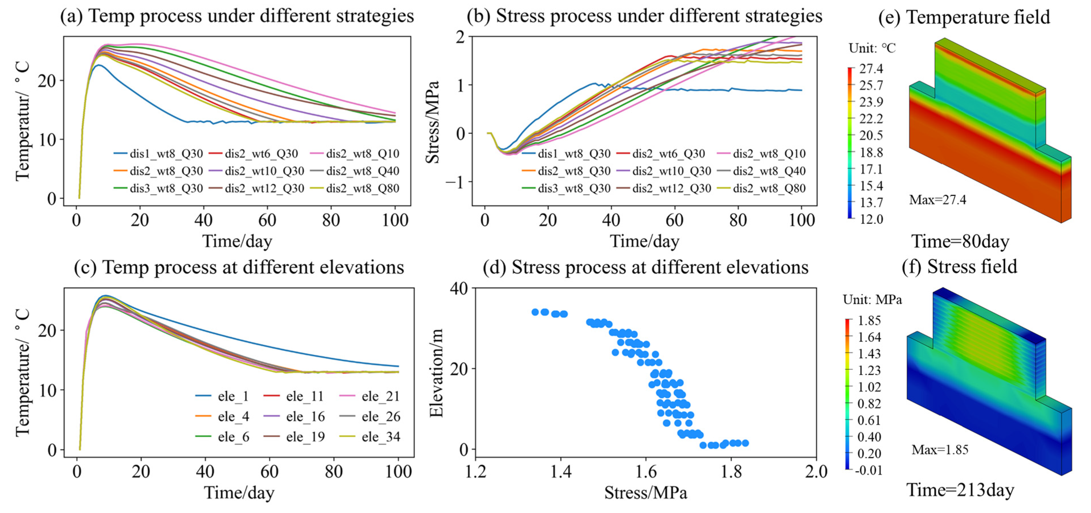
4.1.3. TSSM Validation

The thermodynamic coupling calculation in the TSSM reveals a significant regularity in the spatiotemporal evolution of temperature and stress. In the temporal dimension, the thermodynamic properties of the material interact with the cooling system, thus influencing the efficiency of temperature and stress evolution. In the spatial dimension, factors such as structural restraints, cooling process, and boundary conditions collectively determine the spatial distribution of temperature and stress fields. Consequently, the analysis focuses on the regional node or element within each casting block that experiences the maximum thermal stress. This analysis aims to investigate the evolution of temperature stress under different strategies and the spatial distribution of stress under the same strategy.

Temperature Response Under Different Cooling Strategies

The temperature response under various cooling strategies is presented in Figure 7a, demonstrating the significant influence of water pipe spacing, water temperature, and flow rate on the temperature process, particularly the overall temperature gradient and cooling efficiency. In the figure, dis1 indicates a water pipe spacing of 0.5 m, wt8 represents a cooling water temperature of 8 °C, Q30 corresponds to a cooling flow rate of 30 m³/d, and so forth for other cases. The response characteristics of different strategies are summarized as follows:

(i) Increasing the cooling water pipe spacing from 0.5 m to 1.5 m for a flow rate of 30 m³/d and a water temperature of 8 °C notably reduces the cooling efficiency. The maximum temperatures of the concrete units reach 22.5 °C, 25 °C, and 26.1 °C, with corresponding times to reach the target temperature of 37 d, 71 d, and 100 d, respectively. These results emphasize the significance of water pipe spacing in reducing temperature peaks and enhancing cooling efficiency.

(ii) Figure 7a indicates that when the water pipe spacing remains at 1 m and the flow rate remains at 30 m³/d, the cooling efficiency gradually declines with an increase in water temperature from 6 °C to 12 °C. Each 2 °C rise in water temperature leads to approximately a 1 °C increase in the maximum temperature of the casting unit and prolongs the time to reach the target temperature to 58 d, 70 d, 84 d, and 100 d. This observation demonstrates that higher cooling water temperatures correspond to more pronounced decreases in cooling efficiency, with longer durations required when approaching the target temperature.

(iii) When the water pipe spacing is fixed at 1 m and the water temperature is at 8 °C, increasing the flow rate results in higher maximum temperatures of the casting unit and improved cooling efficiency, albeit with a clear nonlinear characteristic. Elevating the flow rate from 10 m³/d to 80 m³/d reduces the maximum concrete temperature by 3 °C and shortens the cooling time from over 100 d to 58 d, nearly doubling the cooling efficiency. However, increasing the flow rate from 40 m³/d to 80 m³/d only reduces the cooling time by 6 days and improves the cooling efficiency by a mere 7%. This finding aligns with the limited thermal conductivity of concrete. Consequently, while adjusting the flow rate can effectively regulate the temperature, there exists an efficiency threshold for flow rate regulation. Selecting an appropriate flow rate is crucial for cost control, further highlighting the significance of the optimization strategy explored in this paper. In conclusion, the mechanism model can accurately simulate the temperature response over time under different strategies.

Stress Response Under Different Cooling Strategies

The stress response under different cooling strategies is depicted in Figure 7b, highlighting the direct influence of temperature history and temperature control strategies on thermal stress. This, in turn, affects cooling efficiency, structural safety, and material quality benefits. The findings can be summarized as follows:

(i) Enhancing cooling efficiency contributes to the full development of early material performance and improves long-term structural safety. A comparison between strategy dis2_wt6_Q30 (strategy 1) and dis2_wt10_Q30 (strategy 2) reveals maximum temperatures of 24.48 °C and 25.17 °C, respectively, with corresponding times to reach the target temperature of 13 °C being 62 d and 87 d. It is evident that although the total temperature gradient differs by only 2%, strategy 1 demonstrates a 40% improvement in cooling efficiency compared to strategy 2. Furthermore, assessing safety considerations, the maximum stresses for strategy 1 and strategy 2 amount to 1.597 MPa and 1.881 MPa, respectively, indicating that the overall safety of strategy 2 is 17% lower than that of strategy 1. Examining the stress process, we can see that strategy 1 exhibits higher early stress levels due to its rapid cooling rate. However, the material properties can fully develop upon reaching a stable temperature, owing to the rapid growth of early hydration strength in concrete. In contrast, strategy 2 yields higher final stress levels despite lower early stress, which is not conducive to the long-term operational safety of the structure. As the concrete strength increases, stress further escalates under the same temperature drop gradient. Additionally, strategy dis2_wt6_Q30 demonstrates a slight stress decrease after reaching the peak, indicating that the material’s creep relaxation effect can further enhance structural safety.

(ii) Different combinations of cooling strategies can achieve the same stress effect, but there are notable cost differences. Comparing scheme dis2_wt6_Q30 (strategy 1) and dis2_wt8_Q80 (strategy 3), maximum temperatures of 24.48 °C and 24.26 °C, and maximum stresses of 1.597 MPa and 1.514 MPa, respectively, are observed. The time required to reach the target temperatures is 62 d and 58 d, respectively. The safety difference between the two strategies is merely 5.2%, while the cooling efficiency differs by 6.4%. However, the flow rate of strategy 2 is 2.7 times that of strategy 1, and the temperature of strategy 1 is 0.75 times that of strategy 2. Consequently, although the cooling effect is the same, there is clearly a more balanced choice if the cost of cooling and pressurization of water is taken into account.

In summary, the presented content effectively addresses the stress response under different cooling strategies.

Temperature and Stress Response at Different Elevations Under the Same Cooling Strategy

The temperature response of the structure at different elevations under the same cooling strategy is depicted in Figure 7c. It can be observed that the temperature variation exhibits spatial variability, which is influenced by the construction sequence and the temperature of the underlying bedrock. By considering strategy 3(dis2_wt8_Q80) as the reference, the temperature variation process in the central region of casting units at different elevations is investigated. It is evident that the bottommost concrete block is significantly influenced by the ground temperature, leading to lower cooling efficiency. However, as the height reaches 6 m, the impact of heat transfer from the bedrock becomes negligible. In practical engineering projects, there are minor temperature fluctuations among different pouring units due to variations in the temperature of newly poured concrete at the upper levels and the pre-existing concrete at the lower levels. As shown in the figure, the difference in cooling efficiency and maximum temperature of different pouring units with the same cooling strategy does not exceed 5% for elevations over 6 m.

Under the same cooling strategy, the stress response of the structure at different elevations is shown in Figure 7d. It can be observed that there is a significant spatial variation in temperature-induced stress, indicating a strong influence of structural restraints on stress. Taking strategy 3 as the reference, it can be seen that the stress level decreases as the height increases, exhibiting distinct nonlinear characteristics. In the region close to the bedrock, the stress level is high. When the height reaches approximately 30 m, there is a noticeable decreasing trend in stress, suggesting the presence of a turning point. As mentioned in Section 3.1, the height of the constrained zone is related to the length of the casting block, with each casting block having a length of 80 m. The results indicate that the height of the constrained zone is approximately 30 m, which corresponds to about 0.35 times the length of the casting unit. As mentioned earlier, the cooling process of the casting units at elevations of 11 m and 34 m is essentially the same, but the maximum stress levels are approximately 1.35 MPa and 1.60 MPa, respectively, with a difference of over 41%. Therefore, when selecting strategies, it is necessary to consider the spatial restraints of the structure to ensure that the chosen strategy meets safety requirements.

Structural Space Temperature and Stress Response

The distribution of the typical temperature field and stress field is shown in Figure 7e,f, respectively. It can be observed that understanding the distribution patterns of temperature and stress in massive concrete structures can provide more accurate support for constructing the dataset of surrogate models. From the temperature contour map, it can be seen that the concrete blocks gradually cool down from the bottom to the top. The middle section of the block has the highest temperature, while the temperature at the interface with the air is relatively lower. However, due to the poor thermal conductivity of concrete and the application of polyurethane spray as an insulation material on the surface of the dam, the influence of the air temperature boundary on the internal temperature is limited to a depth of no more than 0.5 m. Therefore, the focus is mainly on the internal temperature.

In the stress contour map, when all the blocks reach the target temperature (time = 213 d), the overall temperature field becomes uniform, and the overall stress level of the structure is highest at this point. The stress in the structure gradually decreases from the bottom to the top, with the maximum stress occurring in the middle section of the block. This provides support for selecting representative data points for the surrogate model. By choosing the area with the maximum stress in each block as a representative, the effectiveness of the data can be significantly improved, and the number of data required for the dataset can be greatly reduced.

In summary, the established mechanism model can simulate the temperature and stress processes throughout the entire duration of massive concrete structures. Through computational analysis, the temporal–spatial evolution mechanisms of temperature and stress in concrete arch dams under different cooling strategies are revealed, providing both mechanism understanding and data support for surrogate models.

4.2. Surrogate Model for Arch Dams

Based on the characteristics of cooling systems in engineering, an orthogonalized generation strategy dataset is created to train and validate the surrogate model. Section 4.1 reveals the temporal and spatial evolution characteristics of temperature and stress under different strategies through sensitivity analysis of the mechanistic model. Therefore, the cooling strategy, residual hydration heat of materials, structural spatial restraints, and time effects are selected as four important features for the input of the surrogate model, while structural stress and temperature responses are chosen as output features to construct the model.

4.2.1. Dataset Generation

The quality and quantity of the data are crucial to ensure the accuracy of the model. The construction of the dataset should adhere to the principle that the generated cooling strategy combinations cover all possible cooling states, while also ensuring that the material performance parameters are derived from actual engineering and testing. Figure 8 illustrates the categorization of input parameters generated through orthogonalization into four categories:

(i) Cooling-strategy generation takes into consideration the working capacity of the cooling system and the convenience of site construction. The cooling water pipe spacing (CSdis) is selected as 0.5 m/1.0 m/1.5 m, the cooling water temperature (CSwt) ranges from 6 to 14 °C, and the cooling flow rate (CSQ) is set at 2~80 m³/d.

(ii) The residual heat of hydration ($M_{rhh}$) is calculated as a time-dependent term using Equation (14). For the Baihetan Project, the adiabatic temperature rise value of LHC concrete is determined as 26 °C, and the hydration exothermic coefficient, m, is 0.39, based on the inversion of parameters from massive concrete adiabatic temperature-rise tests and field-monitoring data.

(iii) Based on the findings in Section 4.1, the structural restraint effect is positively correlated with the change in elevation. In this paper, elevation (Zlocation) is used as the characterization index of the restraint degree. This approach offers a more straightforward way to characterize the complex structural restraint degree, considering the restraint effect and avoiding the difficulty in solving the calculation formula [14] for the restraint degree. Moreover, it enables the direct determination of stress variation along the elevation direction, providing the possibility of a full-domain stress evaluation and effectively improving the training accuracy of the surrogate model.

(iv) The time effect of the strategy (CStime) is utilized to evaluate the response of temperature and stress over time, starting from the concrete pouring of the dam block. Two types of output parameters are obtained by developing an automated calculation and post-processing program based on Python and TSSM: (i) structural stress response (SR_stress) and (ii) structural temperature response (SR_temp).

The cooling strategy equivalent to the casting block is depicted on the left side of Figure 8, and the dataset, consisting of 2,340,260 samples, is generated by orthogonalizing the aforementioned interval. A correlation analysis between the input and output features of the dataset reveals the following findings: (i) a clear correlation exists between the input and output features, indicating a well-founded selection of features for the surrogate model; (ii) the influence of the input features on the output features exhibits complex nonlinearity, aligning with the conclusion drawn in Section 4.1, wherein the flow rate, water temperature, time, and space constraints exert varying degrees of influence on the structural response; and (iii) the stress and temperature levels exhibit significant variations across different input features, demonstrating the representativeness and generalizability of the dataset. In summary, the generated strategy combinations encompass all possible limit states, offering a wide-area feasible solution space for the optimization model.

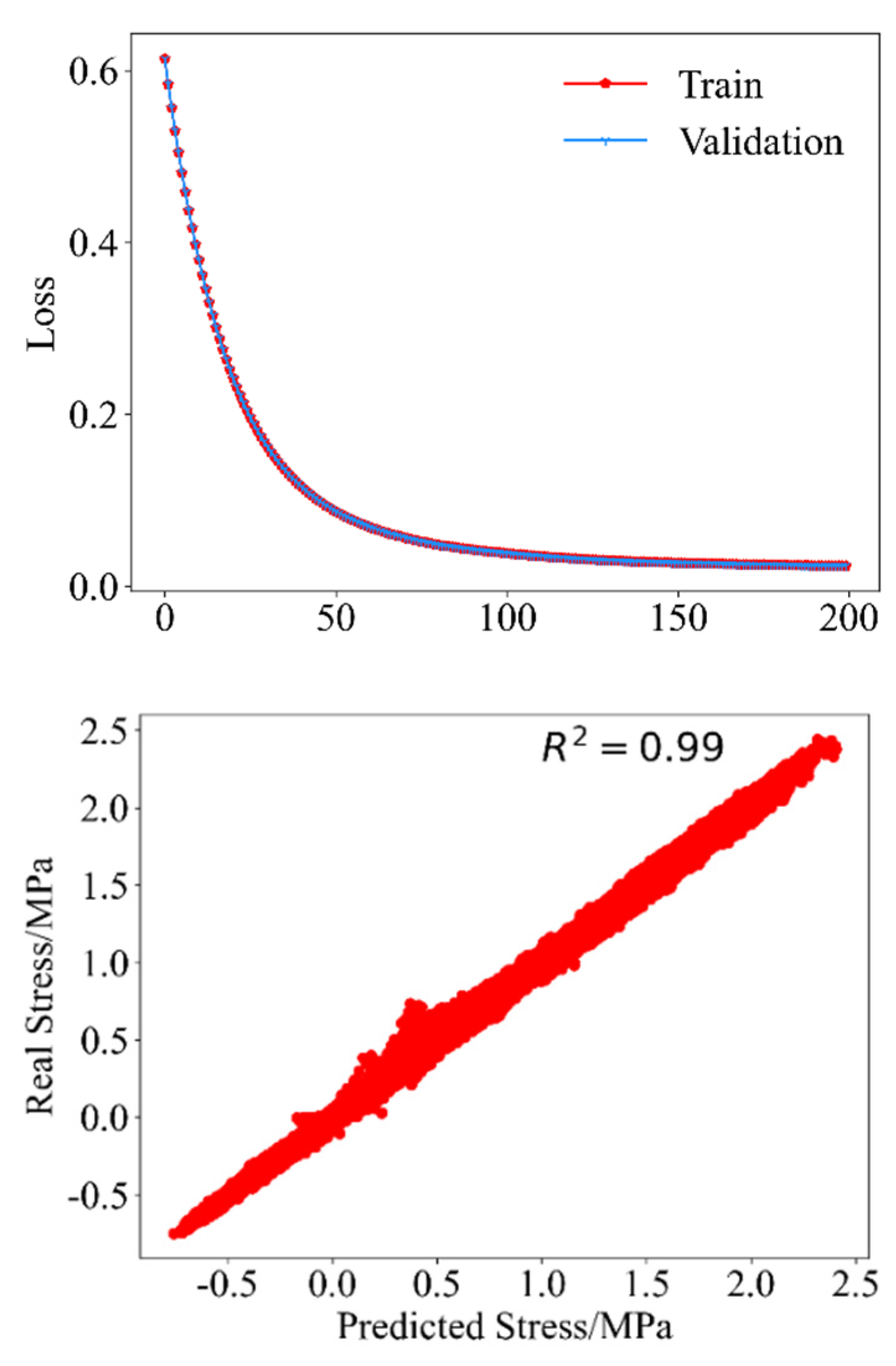
4.2.2. Model Training

The parameters and hyperparameters of the surrogate model directly impact the efficiency and accuracy of model training. Therefore, suitable model parameters were selected through sensitivity testing to mitigate overfitting and underfitting issues. Specifically, the model type is set as gbtree, with a maximum tree depth of 10, pruning parameter of 0.1, subsample ratio of training samples of 0.8, L2 regularization parameter of 10, L1 regularization parameter of 0, learning rate of 0.1, squared error as the loss function for regression tasks, rmse as the model evaluation metric, and a total of 200 training rounds.

The dataset is split into 80% for training and 20% for testing. As illustrated in the left plot of Figure 9, the loss on the test set and validation set rapidly decreases within the first 100 rounds, and the loss curve converges when reaching 200 training rounds. The RMSE on the training set is 0.02134, while on the validation set, it is 0.02158. The loss curve demonstrates a consistent performance between the training and test sets, indicating a lack of overfitting or underfitting. In the bottom plot of Figure 9, a scatter plot of 400,000 samples in the validation set shows an R² value of 99%, indicating a prediction accuracy of 99%. Section 4.2.3 and Section 4.2.4 of this paper will further validate the model and discuss its interpretability.

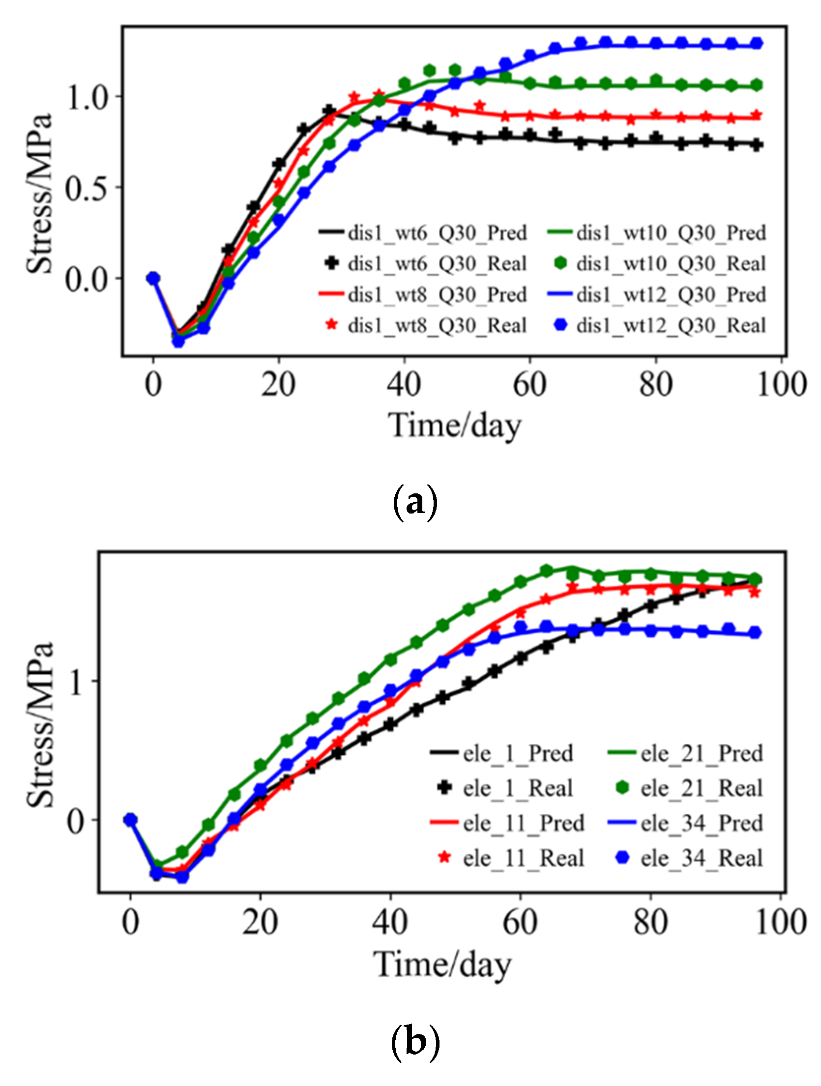
4.2.3. Model Validation

The comparison between the results obtained from the mechanistic model and the predictions generated by the surrogate model is conducted from both temporal and spatial perspectives, as illustrated in Figure 10. From a temporal viewpoint, the predicted stresses by the surrogate model exhibit a high degree of similarity to the actual calculated stress process, with nearly identical timing and numerical values for the maximum compressive stress, maximum tensile stress, and final stress level. Figure 10a demonstrates that despite notable variations in the stress process under different cooling strategies, such as when the spacing is 0.5 m, the flow rate is 30 m³/d, and the water temperature ranges from 6 °C to 12 °C, the mechanistic model predicts maximum stresses of 0.732 MPa, 0.903 MPa, 1.056 MPa, and 1.296 MPa, while the surrogate model predicts maximum stresses of 0.742 MPa, 0.877 MPa, 1.050 MPa, and 1.273 MPa, with an average prediction error of less than 2%. Furthermore, the surrogate model accurately captures the timing of the occurrence of maximum compressive and tensile stresses, corroborating the findings of the mechanistic model. Additionally, the stress evolution can be divided into two stages. In the first stage, referred to as the cooling strategy regulation stage, a significant range of stress variation is observed. In the second stage, when the structural temperature reaches the target temperature, the stress level reaches its peak and gradually decreases due to temperature uniformity and the minimal effect of creep. By examining the “dis1_wt8_Q30” strategy in the figure, it is evident that the surrogate model not only accurately depicts stress changes throughout the first stage but also learns the creep characteristics of the structure through a substantial number of data. This capability is of paramount importance for evaluating the construction and long-term operational safety of the structure. It signifies that the surrogate model can effectively predict stress levels throughout the entire process and accurately estimate stress during the complete cooling process of various casting blocks under different strategies, thereby offering support for comprehensive time optimization.

From a spatial perspective, the surrogate model accurately reflects stress distribution patterns at different elevations, as depicted in Figure 10b. Specifically, under the “dis2_wt8_Q30” strategy, stress profiles at four representative elevations (1 m/11 m/21 m/34 m) are selected and displayed in Figure 10b. The stress levels are higher in proximity to the bedrock and decrease as the distance from it increases. The surrogate model predicts maximum stresses of 1.746 MPa, 1.696 MPa, 1.817 MPa, and 1.392 MPa, respectively, at these elevations. In comparison to the mechanistic model, the prediction errors are 0.05%, 0.001%, 1.42%, and 1.56%, resulting in an average error within 2%, consistent with the findings in Section 4.2.2. These results indicate the surrogate model’s effectiveness in replacing and predicting spatial stress distribution along the elevation direction, thereby supporting comprehensive spatial optimization.

In summary, the dual-driven surrogate model, based on mechanistic data, enables accurate and efficient evaluation of structural responses under various strategies. By generating cooling strategies through the orthogonalization of performance parameters within the engineering cooling system and constructing a large-scale dataset, the surrogate model exhibits strong generalization capabilities. It achieves both high prediction accuracy and broad coverage of strategies. The accuracy and interpretability of the surrogate model have been validated against the mechanistic model. Consequently, a surrogate model that meets accuracy requirements will provide precise and efficient evaluation support for multi-objective optimization models.

4.2.4. Model Interpretability

Interpretability holds significant importance in data models, necessitating the evaluation of surrogate models using the SHAP method in conjunction with practical engineering scenarios. The fundamental concept of the SHAP method involves quantifying the marginal contribution of each feature to the model’s output and providing explanations for “black box models” at both the global and local levels. SHAP establishes an additive explanation model that considers all features as contributors. In this section, SHAP values are computed for a dataset comprising 1.8 million training samples, and the significance and influence range of different features are analyzed and summarized in Figure 11. Specifically, the feature determines the position on the y-axis, while each Shapley value determines the position on the x-axis. A larger SHAP value indicates a greater impact of the feature on the output, and it also signifies whether the feature has a positive or negative effect on the output.

According to Figure 11a, the residual heat of hydration is the most impactful feature on stress, followed by cooling strategies encompassing cooling flow rate, distance between cooling pipes, and cooling water temperature. Lastly, the influence of structural spatial restraints is considered. (i) Further analysis demonstrates that the time-varying residual heat of hydration is the dominant factor in temperature stress. It encompasses both the hydration characteristics of concrete and time-dependent factors, acting as the primary positive heat source and playing a commanding role in temperature stress. (ii) Among the cooling strategies, the cooling flow rate has a greater impact on temperature stress compared to the distance between cooling pipes and cooling water temperature. This can be attributed to the wider adjustable range of the cooling flow rate, which provides enhanced stress regulation capabilities. This finding aligns with practical engineering scenarios. The regulation of flow rate can be achieved by adjusting pipe pressure and valve size, while controlling water temperature or adjusting the distance between cooling pipes is more challenging and involves a certain time lag. This further underscores the crucial role of flow rate regulation in strategy control. (iii) Spatial positioning also holds significance, but its influence on stress is lower than that of cooling strategies. Two key reasons account for this observation. Firstly, based on relevant literature on concrete confinement effects, the height of the strong confinement zone is approximately 0.25–0.35 times the length, corresponding to a height range of 20–30 m. Once outside this confinement zone, the influence diminishes. Therefore, spatial restraints possess a local characteristic. On the other hand, cooling strategies exhibit global characteristics, leading to a more pronounced impact on the results compared to spatial restraint effects. This concurs with practical engineering situations.

According to Figure 11b, different features exhibit varying positive and negative contributions to stress. Specifically, (i) when the residual heat of hydration is high, its impact on stress is relatively small, as indicated by the dominant red portion in the figure. This occurs because a higher residual heat of hydration signifies the early cooling stage, where the primary factor is the heat released during concrete hydration. During this stage, the temperature increases, leading to an augmentation of compressive stress and a reduction in tensile stress, thereby displaying a negative correlation with the final stress. As the residual heat of hydration gradually decreases, the concrete strength experiences rapid growth. In comparison to the initial stage, the same cooling gradient induces a greater generation of stress. Consequently, in the later cooling stage, the SHAP value of the residual heat of hydration decreases, while its impact on stress significantly increases, as depicted by the blue section in the figure. In the intermediate stage, spanning from the temperature increase phase to the second zero-stress phase, the SHAP value of the residual heat of hydration gradually declines, transitioning from red to blue, as shown in the figure, thereby revealing a strong regularity. For the specific case under consideration, the overall cooling gradient ranges from 10 to 14 °C, typically resulting in a cooling range of 5–7 °C from the highest temperature to the second zero stress. This alignment corresponds with the actual evolution of temperature-induced stress in engineering practice. Thus, the effect of this feature remains consistent with practical engineering. (ii) Concerning cooling strategies, flow rate, distance, and water temperature interact with one another. Analysis of the SHAP values reveals that a higher flow rate contributes more to stress adjustment, indicating that an increase in flow rate affects stress adjustment. Lower cooling water temperature leads to greater stress, while the effect of pipe distance is relatively balanced. This balance is associated with the equilibrium between flow rate and water temperature under different distances. (iii) Analysis of the spatial restraint characteristics demonstrates that higher SHAP values correspond to smaller positive effects on stress. This observation indicates a reduced correlation between stress level and elevation outside the confinement zone. When the SHAP value is lower, the positive effect on stress becomes more pronounced. From the uniformly distributed SHAP values of the samples, it can be observed that the confinement zone and non-confinement zone account for an equal proportion of 50%. This suggests that, in this case, the elevation of the confinement zone is approximately 16 m, consistent with the literature’s indication of 0.2–0.25 times the block length (L) [1].

In summary, it shows that the features selected based on the mechanism are reasonable and the surrogate model has strong interpretability. Therefore the model is reliable and accurate and can be used for optimization.

4.2.5. Comparative Discussion of Surrogate Model and Mechanism Model

Compared with the mechanistic model, the surrogate model has a greater advantage in terms of computational efficiency and model size. In terms of time, the trained surrogate model takes only 0.084 s to predict the stress response of 12 casting blocks, while the mechanical model takes 591 s to calculate a single cooling strategy (excluding post-processing time), which is 7000 times more efficient than the mechanical model. Theoretically, the trained surrogate model can almost immediately obtain the stresses under any combination of strategies and evaluate the spatiotemporal safety with much higher efficiency than the mechanistic model, thus providing the possibility for large-scale optimization.

In terms of model size, the mechanism model for a single cooling strategy includes calculation and result files of more than 817 MB, and the data size of calculation results for hundreds of strategies is very large, which is not easy to store and query quickly. In contrast, the pre-trained agent model is only 11.8 MB, which is very small, making it easy to deploy and migrate applications online. Therefore, the MS-SM has an important prospect in intelligent construction.

In summary, the mechanism data-driven surrogate model (MD-SM) was established by evaluating the importance features, selecting a suitable algorithm, and constructing a high-quality dataset, and the accuracy, efficiency, and interpretability of the model were comprehensively tested. The surrogate model not only reveals the relationship between key factors and the spatiotemporal response of the structure, but also achieves an accurate and rapid evaluation of the effects of different cooling strategies on the spatiotemporal stress of the structure.

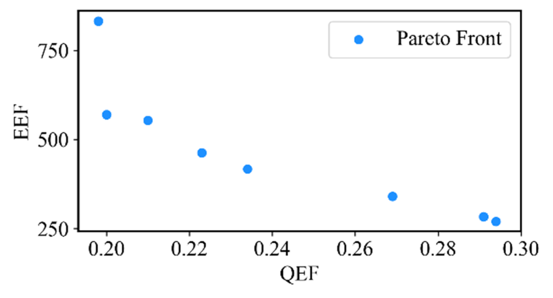
4.3. Optimization Model

The objective of the optimization model is to obtain the Pareto solution set for cooling strategies that achieve a balance between safety, quality, and efficiency. In practical engineering, the QEF design requires a minimum safety factor ($k^d$) of 2.0. The SEF defines $t^{final}$ as the time when cooling reaches the target temperature and stress reaches its maximum value, which is obtained through the surrogate model.

The parameters of the NSGA-II algorithm in the optimization model can be adjusted based on the ideal balance between exploration and exploitation in the specific problem domain and search space. In this study, the selected parameters are as follows: the population size is set to 50, which represents the number of individuals in each generation of the population. As the evolution progresses, the number of individuals that meet the requirements increases, generating multiple optimization strategies. The maximum number of generations is set to 500, which represents the maximum number of times the algorithm will run before stopping. The chromosomes are encoded using binary encoding (BG). The crossover probability is set to 0.6, which represents the probability of crossover occurring during the reproduction process. The mutation probability is set to 0.01, which represents the probability of gene mutation during the reproduction process. Choosing a small value for the mutation probability can avoid significant disruption to the population and ensure the exploration of new solutions. The tournament selection pressure is set to 2, which indicates the degree to which better individuals are favored over poorer individuals during the tournament selection process. The crowding distance is represented by the Euclidean distance, which is used to calculate the distance metric of individual density in the population. The crowding factor is set to 1.5, which is a threshold for determining whether two individuals are too close and need to be separated.

The optimization results, depicted in Figure 12, were obtained by minimizing the optimization objectives of QEF and EEF. Through multiple experiments and 250 iterations, the results converged and exhibited robustness. In the computational process, a set of cooling strategies that achieve a balance between safety, quality, and efficiency (S-Q-E) was derived by evaluating a total of 50 × 250 strategies. The entire computation process lasted for 23 min.

4.4. Decision Model

The objective of a multi-criteria decision-making model is to identify the most cost-effective solution from the Pareto set that fulfills safety, quality, and efficiency criteria, taking into account the cost characteristics associated with the design and operation of the cooling system. Initially, the methodology for the decision-making model is established. Subsequently, appropriate cost-benefit evaluation indicators are selected. Lastly, the decision-making model is employed to derive the optimal balanced strategy, which is then compared with conventional strategies.

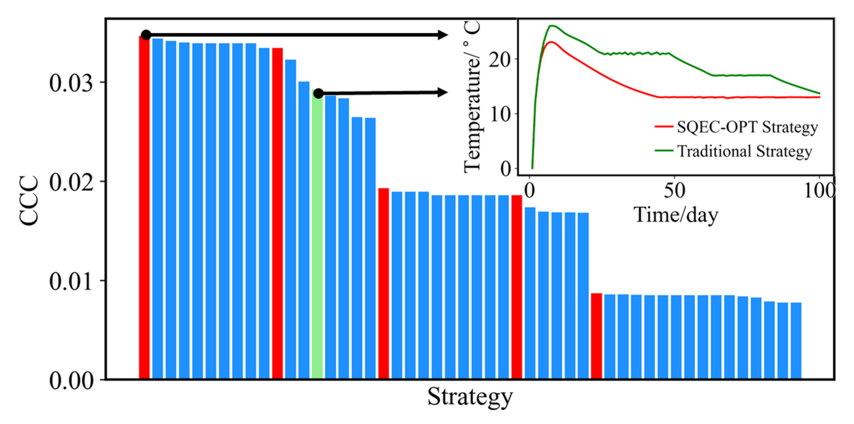
4.4.1. Strategy Comparison

The decision criteria for the Baihetan Project were established by considering the actual circumstances, as discussed in Section 3.4. Among these criteria, the water pipe spacing aims to maximize cost reduction by increasing the spacing. Conversely, the cooling water flow rate aims to minimize costs by reducing the flow rate. The analysis in Section 4.1.3 reveals that beyond a certain threshold, increasing the cooling flow rate does not significantly enhance cooling efficiency but leads to higher expenses. Thus, an appropriate flow rate contributes to cost savings. The cooling water temperature serves as an intermediate criterion. The target temperature for the casting blocks is 13 °C, and the cooling units have the capability to maintain the water temperature between 6 °C and 14 °C. For the Baihetan Project, a water temperature around 10 °C is the most economically advantageous. Additionally, the cooling time is considered an interval-type criterion. Based on Formula (13b), which examines the tensile strength of low-heat cement concrete in the Baihetan Project, the material typically achieves 80% to 90% of its strength within 50 to 60 days. Gao et al. conducted strength tests on fully graded concrete and wet-screened concrete specimens from the Baihetan Dam at 28 and 90 days, further confirming this finding [55]. Therefore, controlling the cooling time within the range from 50 to 60 days ensures optimal material performance (i.e., reaching the peak stress when the strength reaches 90%) and guarantees economic efficiency. It should be noted that the cooling time is provided by the surrogate model.

Based on the given criteria, the TOPSIS method was applied to normalize each index and determine both the positive and negative ideal solutions. Subsequently, the distances from each candidate solution to the ideal and negative ideal solutions were calculated. Based on these calculated distances, the cooling comprehensive cost (CCC) index was used to measure the similarity between each candidate solution and the optimal solution. The 50 solutions that met the safety, quality, and efficiency criteria were then ranked according to their CCC values, as shown in Figure 13. The strategy with the highest CCC score, namely S8, represents the optimal balance among safety, quality, efficiency, and cost. The traditional cooling strategy, represented by the green scheme (Strategy 8, S8), is depicted in the top right corner of the image, along with the typical temperature profiles of the optimal and traditional strategies. Selected solutions (marked in red in the figure) were compared and analyzed, and the specific parameters of the strategies are provided in

Table 4. Typical strategies.

Strategy (ID)	CSdis (/m)	CSwt (/°C)	CSQ/(m3/d)	Cstime (/Day)	CCC
S8	0.6	9.80	32.46	56.9	0.035
S44	0.6	9.05	32.49	56.9	0.033
S49	1.5	8.00	30.00	90.0	0.029
S3	0.6	12.34	47.91	83.2	0.019
S23	0.5	12.34	47.92	83.2	0.019
S27	0.7	6.21	67.93	28.3	0.009

.

(i) Comparing S8 and S44, it can be observed that the cooling water pipe spacing, flow rate, and time required to reach the target temperature are essentially the same in both strategies. However, there is a slight difference in the cooling water temperature of 0.75 °C, indicating that the S44 scheme is slightly less cost-effective than the S8 scheme.

(ii) When comparing S8 with S3 and S23, it becomes apparent that although the water pipe spacing is similar in these schemes, the cooling water temperature is higher in S3 and S23. Consequently, achieving the desired cooling temperature requires an increase in the flow rate. While raising the water temperature by 2.54 °C can reduce cooling costs, it also leads to a longer overall cooling time. As a result, the overall cost increases by 84% compared to the S8 solution, aligning with the real-world scenario of higher costs due to extended durations.

(iii) In the comparison between the S49 scheme and the S23 scheme, it is evident that although the cooling efficiency of the S23 scheme improves by 8%, the cooling water pipe spacing in the S49 scheme is three times that of S23, and the flow rate is only 62.6% of the S23 scheme. Despite the S49 solution having a cooling water temperature 4 °C higher than the S23 solution, the overall cost is reduced by 50%. Drawing from engineering experience, increasing the spacing of cooling water pipes by a factor of two can result in material savings, as both horizontal and vertical spacing are increased simultaneously. Moreover, the increased pipe spacing reduces construction complexity and labor costs. Thus, the decision model effectively evaluates the advantages and disadvantages of the strategies.

(iv) Comparing S8 with S27, it is evident that S27 employs a very low water temperature and a higher flow rate to achieve a significantly high cooling efficiency, aligning with the objective of maximizing the efficiency of the optimization model. However, the low water temperature and high flow rate lead to poor economics in this strategy. Additionally, from a practical standpoint, the low cooling water temperature results in a large temperature gradient around the water pipe, increasing the risk of cracking. Therefore, despite meeting the requirements for safety and efficiency, this solution is not a balanced one.

4.4.2. Optimization Strategy Versus Traditional Strategy

The present study compares the balanced strategy with the traditional strategy by evaluating the traditional strategy (S49) within the decision model and conducting a preliminary comparison with the balanced strategy (S8). Figure 13 demonstrates that the traditional strategy also exhibits favorable performance among the various options. In the figure, the red bars in the figure are used to highlight strategies that exhibit significant differences in performance (CCC value) compared to other strategies. In order to comprehensively evaluate the optimal strategy obtained through the SQEC-TSOM method, a comparative analysis will be conducted between the balanced strategy and the traditional strategy in terms of temperature and stress evolution in both time and space, as depicted in Figure 14.

(i) Evaluation of cooling efficiency: Since there was a total of 12 casting units with a 7-day interval, all units were cast by day 84. By the time it reached day 90, the last casting unit had been cooled by water for 6 days and had just reached the peak temperature, as shown in Figure 14. More than 2/3 of the casting block under the balanced strategy have successfully reached the target temperature, while the casting block at the bottom of the traditional strategy has not yet fully reached the target temperature and is still in the cooling stage. The balanced strategy exhibits a smaller and more uniform temperature gradient compared to the traditional strategy. By day 213, both the balanced strategy and the traditional strategy have reached a stable temperature field, exhibiting a relatively consistent temperature distribution in space. Figure 13 presents the typical temperature profiles at an elevation of 11 m, revealing maximum temperatures of 23.08 °C and 26.06 °C for the balanced strategy and the traditional strategy, respectively. The balanced strategy results in a 30% reduction in the total temperature gradient, and the time required to cool to the target temperature is 49 days and 100 days for the balanced strategy and the traditional strategy, respectively. Consequently, the cooling efficiency is doubled under the balanced strategy. Further analysis showed that the total time to cool the 12 pouring units to a stable temperature for the optimized strategy was 136 days, compared to 213 days for the conventional strategy, resulting in a 36% improvement in cooling efficiency for the entire project.

(ii) Safety evaluation: When the dam structure reaches a stable temperature field, its overall stress level reaches its peak and subsequently stabilizes. Analysis of stress cloud map in Figure 14 reveals that the balanced strategy exhibits a lower overall stress level and a more uniform stress distribution in space compared to the traditional strategy. It is evident that the traditional strategy experiences significant tensile stress at its central internal region, rendering it susceptible to the development of internal detrimental cracks rather than surface cracks. This observation aligns with the failure mechanism observed in massive concrete structures under thermal loading. Specifically, the bottommost region with strong restraints exhibits higher tensile stress. The balanced strategy, with its high cooling efficiency, achieves the target temperature earlier, leading to a gradual reduction in tensile stress due to creep. Moreover, influenced by the temperature of the underlying bedrock, the temperature of the bottom concrete experiences a slight rise, further diminishing the stress level in the strongly constrained region. Thus, it is evident that the tensile stress at the bottom is lower than that at the top under the balanced strategy. This signifies the effective risk reduction associated with the balanced strategy compared to the traditional approach. An examination of the stress cloud map in Figure 14 indicates a maximum stress of 1.26 MPa for the balanced strategy, while the traditional strategy records a maximum stress of 1.80 MPa. This suggests that the safety level during operation is 42% higher for the balanced strategy than for the traditional strategy.

(iii) Evaluation of material performance: Analysis of the stress–strain curves depicted in Figure 15 reveals a strong correlation between the stress development of the balanced strategy and the early-stage strength development curve. This alignment enables the comprehensive utilization of material growth characteristics. Moreover, the average duration of temperature control for the balanced strategy is 56.9 days, aligning consistently with the time required for LHC concrete to achieve 90% of its strength.

(iv) Assessment of cost-effectiveness of cooling strategies: Both the balanced strategy and the traditional strategy employ a cooling flow rate of 30 m³/d, while maintaining cooling water temperatures of 10 °C and 8 °C, respectively, in accordance with the actual on-site conditions. The cooling water pipe spacing for the balanced strategy is set at 0.6 m, which plays a crucial role in ensuring safety and efficiency through the utilization of higher water temperatures and reduced flow rates. Notably, the temperature-control technical regulations for the Baihetan arch dam state that the cooling water pipe spacing can be reduced to 0.5 m in scenarios where temperature control is challenging or when high safety requirements are necessary. This provision affirms that the balanced strategy aligns effectively with practical conditions. Furthermore, the CCC for the balanced strategy and the traditional strategy are 0.035 and 0.029, respectively, indicating that the balanced strategy can achieve an approximate 20.6% cost reduction compared to the traditional strategy.

In conclusion, the SEQC-balanced strategy proves to be effective in enhancing structural safety, optimizing material performance, improving cooling efficiency, and reducing overall costs. Moreover, it facilitates the efficient management of temporal–spatial thermal stress in complex massive concrete structures.

5. Conclusions

This study introduces the Safety–Quality–Efficiency–Cost Thermal Stress Optimization Method (SEQC-TSOM), an innovative approach for intelligent thermal stress management in large concrete structures. By integrating both mechanistic insights and data-driven analysis, SEQC-TSOM efficiently identifies optimal cooling strategies, facilitating spatiotemporal optimization of thermal stresses. Through a case study, the method’s effectiveness in balancing safety, efficiency, and cost is demonstrated. Key achievements include the following:

(1) The development of a comprehensive Thermal Stress Simulation Mechanism Model (TSSM) that enables precise analysis of thermal stress throughout complex concrete structures, aiding in the optimization process. This model effectively simulates temperature and stress evolution under various cooling strategies, uncovering the temporal and spatial dynamics of thermal stress.

(2) The creation of a dual mechanism- and data-driven surrogate model (MD-SM) that quickly and accurately evaluates structural properties. Sensitivity analysis of the mechanism model identifies crucial inputs and outputs for the surrogate model, which includes cooling strategies, material hydration heat, structural restraints, and timing. This model achieves a remarkable prediction accuracy of 99% and operates 7000 times faster than traditional mechanistic models.

(3) Quantitative evaluation of the surrogate model’s interpretability through SHAP values analysis, highlighting the significant impacts of material hydration heat, cooling strategies, and structural restraints on thermal stress. This provides a novel perspective for effective stress management, suggesting strategies like the use of low-heat cement concrete materials, optimization of cooling strategies, and structural restraint optimization.

(4) The establishment of an Intelligent Optimization Model (IOM) that generates balanced strategies for managing thermal stress, employing a non-dominated genetic algorithm for multi-objective optimization. This model efficiently produces a satisfactory Pareto solution set, laying the groundwork for subsequent decision-making models.

(5) The application of a multi-criteria decision model (MCDM) to select the most balanced and cost-effective cooling strategies, showing a 42% improvement in safety, a 36% enhancement in cooling efficiency, and a 20.6% reduction in cooling costs compared to traditional strategies.

In summary, SEQC-TSOM represents a significant advancement in managing thermal stress in massive concrete structures, offering a systematic and scalable framework for optimizing cooling strategies. Future research will aim to further enhance the model’s precision and efficiency and explore its application to a wider range of structural types, contributing to the development of comprehensive datasets for thermal stress control and integrating advanced analytical techniques for improved model accuracy and interpretability.

References

1. Bofang, Z. Thermal Stresses and Temperature Control of Mass Concrete; Elsevier Inc.: Amsterdam, The Netherlands, 2014. [Google Scholar] [CrossRef]
2. ACI Committee. ACI 207.2R-07 Report on Thermal and Volume Change Effects on Cracking of Mass Concrete; ACI Committee: Farmington Hills, MI, USA, 2007. [Google Scholar]
3. Pesavento, F.; Knoppik, A.; Smilauer, V.; Briffaut, M.; Rossi, P. Numerical Modelling. Thermal Cracking of Massive Concrete Structures. State of the Art Report of the RILEM Technical Committee 254-CMS; Springer: Berlin/Heidelberg, Germany, 2018. [Google Scholar]
4. ACI Committee. ACI 231 Report on Early-Age Cracking: Causes, Measurement, and Mitigation; ACI Committee: Farmington Hills, MI, USA, 2010. [Google Scholar]
5. Li, Y.; Nie, L.; Wang, B. A numerical simulation of the temperature cracking propagation process when pouring mass concrete. Autom. Constr. 2014, 37, 203–210. [Google Scholar] [CrossRef]
6. Tasri, A.; Susilawati, A. Effect of cooling water temperature and space between cooling pipes of post-cooling system on temperature and thermal stress in mass concrete. J. Build. Eng. 2019, 24, 100731. [Google Scholar] [CrossRef]
7. Tasri, A.; Susilawati, A. Effect of material of post-cooling pipes on temperature and thermal stress in mass concrete. Structures 2019, 20, 204–212. [Google Scholar] [CrossRef]
8. Mehta, P.K.; Monteiro, P.J.M. Concrete: Microstructure, Properties, and Materials; McGraw-Hill: New York, NY, USA, 2005. [Google Scholar]
9. Lothenbach, B.; Kulik, D.A.; Matschei, T.; Balonis, M.; Baquerizo, L.; Dilnesa, B.; Miron, G.D.; Myers, R.J. Cemdata18: A chemical thermodynamic database for hydrated Portland cements and alkali-activated materials. Cem. Concr. Res. 2019, 115, 472–506. [Google Scholar] [CrossRef]
10. Wang, L.; Yang, H.; Dong, Y.; Chen, E.; Tang, S. Environmental evaluation, hydration, pore structure, volume deformation and abrasion resistance of low heat Portland (LHP) cement-based materials. J. Clean. Prod. 2018, 203, 540–558. [Google Scholar] [CrossRef]
11. Maruyama, I.; Lura, P. Properties of early-age concrete relevant to cracking in massive concrete. Cem. Concr. Res. 2019, 123, 105770. [Google Scholar] [CrossRef]
12. Zhu, H.; Hu, Y.; Li, Q.; Ma, R. Restrained cracking failure behavior of concrete due to temperature and shrinkage. Constr. Build. Mater. 2020, 244, 118318. [Google Scholar] [CrossRef]
13. Nguyen, D.H.; Nguyen, V.; Lura, P.; Dao, V.T. Temperature-stress testing machine—A state-of-the-art design and its unique applications in concrete research. Cem. Concr. Compos. 2019, 102, 28–38. [Google Scholar] [CrossRef]
14. Xin, J.; Zhang, G.; Liu, Y.; Wang, Z.; Wu, Z. Evaluation of behavior and cracking potential of early-age cementitious systems using uniaxial restraint tests: A review. Constr. Build. Mater. 2020, 231, 117146. [Google Scholar] [CrossRef]
15. Zhu, H.; Li, Q.; Hu, Y.; Ma, R. Double Feedback Control Method for Determining Early-Age Restrained Creep of Concrete Using a Temperature Stress Testing Machine. Materials 2018, 11, 1079. [Google Scholar] [CrossRef]
16. Zhu, H.; Hu, Y.; Ma, R.; Wang, J.; Li, Q. Concrete thermal failure criteria, test method, and mechanism: A review. Constr. Build. Mater. 2021, 283, 122762. [Google Scholar] [CrossRef]
17. Keshavarzi, B.; Kim, Y.R. A dissipated pseudo strain energy-based failure criterion for thermal cracking and its verification using thermal stress restrained specimen tests. Constr. Build. Mater. 2020, 233, 117199. [Google Scholar] [CrossRef]
18. Huang, Y.; Liu, G.; Huang, S.; Rao, R.; Hu, C. Experimental and finite element investigations on the temperature field of a massive bridge pier caused by the hydration heat of concrete. Constr. Build. Mater. 2018, 192, 240–252. [Google Scholar] [CrossRef]
19. Hu, Y.; Zuo, Z.; Li, Q.; Duan, Y. Boolean-Based Surface Procedure for the External Heat Transfer Analysis of Dams during Construction. Math. Probl. Eng. 2013, 2013, 175616. [Google Scholar] [CrossRef]
20. Conceição, J.; Faria, R.; Azenha, M.; Miranda, M. A new method based on equivalent surfaces for simulation of the post-cooling in concrete arch dams during construction. Eng. Struct. 2020, 209, 109976. [Google Scholar] [CrossRef]
21. Ding, J.; Chen, S. Simulation and feedback analysis of the temperature field in massive concrete structures containing cooling pipes. Appl. Therm. Eng. 2013, 61, 554–562. [Google Scholar] [CrossRef]
22. Tatin, M.; Briffaut, M.; Dufour, F.; Simon, A.; Fabre, J.-P. Statistical modelling of thermal displacements for concrete dams: Influence of water temperature profile and dam thickness profile. Eng. Struct. 2018, 165, 63–75. [Google Scholar] [CrossRef]
23. Santillán, D.; Salete, E.; Toledo, M. A methodology for the assessment of the effect of climate change on the thermal-strain–stress behaviour of structures. Eng. Struct. 2015, 92, 123–141. [Google Scholar] [CrossRef]
24. Bažant, Z.P. Prediction of concrete creep and shrinkage: Past, present and future. Nucl. Eng. Des. 2001, 203, 27–38. [Google Scholar] [CrossRef]
25. Rasoolinejad, M.; Rahimi-Aghdam, S.; Bažant, Z.P. Prediction of autogenous shrinkage in concrete from material composition or strength calibrated by a large database, as update to model B4. Mater. Struct. Mater. Constr. 2019, 52, 33. [Google Scholar] [CrossRef]
26. Zuo, Z.; Hu, Y.; Li, Q.; Zhang, L. Data Mining of the Thermal Performance of Cool-Pipes in Massive Concrete via In Situ Monitoring. Math. Probl. Eng. 2014, 2014, 985659. [Google Scholar] [CrossRef]
27. Bofang, Z.; Jianbo, C. Finite Element Analysis of Effect of Pipe Cooling in Concrete Dams. J. Constr. Eng. Manag. 1989, 115, 487–498. [Google Scholar] [CrossRef]
28. Cheng, J.; Li, T.C.; Liu, X.; Zhao, L.H. A 3D discrete FEM iterative algorithm for solving the water pipe cooling problems of massive concrete structures. Int. J. Numer. Anal. Methods Géoméch. 2016, 40, 487–508. [Google Scholar] [CrossRef]
29. Yang, J.; Hu, Y.; Zuo, Z.; Jin, F.; Li, Q. Thermal analysis of mass concrete embedded with double-layer staggered heterogeneous cooling water pipes. Appl. Therm. Eng. 2012, 35, 145–156. [Google Scholar] [CrossRef]
30. Zhong, R.; Hou, G.-P.; Qiang, S. An improved composite element method for the simulation of temperature field in massive concrete with embedded cooling pipe. Appl. Therm. Eng. 2017, 124, 1409–1417. [Google Scholar] [CrossRef]
31. Liu, X.; Zhang, C.; Chang, X.; Zhou, W.; Cheng, Y.; Duan, Y. Precise simulation analysis of the thermal field in mass concrete with a pipe water cooling system. Appl. Therm. Eng. 2015, 78, 449–459. [Google Scholar] [CrossRef]
32. ACI 207.4R-20: Report on Cooling and Insulating Systems for Mass Concrete. Available online: https://www.concrete.org/publications/internationalconcreteabstractsportal.aspx?m=details&id=51729338 (accessed on 9 May 2023).
33. Azenha, M.; Kanavaris, F.; Schlicke, D.; Jędrzejewska, A.; Benboudjema, F.; Honorio, T.; Šmilauer, V.; Serra, C.; Forth, J.; Riding, K.; et al. Recommendations of RILEM TC 287-CCS: Thermo-chemo-mechanical modelling of massive concrete structures towards cracking risk assessment. Mater. Struct. 2021, 54, 135. [Google Scholar] [CrossRef]
34. Kheradmand, M.; Azenha, M.; Vicente, R.; de Aguiar, J.L. An innovative approach for temperature control of massive concrete structures at early ages based on post-cooling: Proof of concept. J. Build. Eng. 2020, 32, 101832. [Google Scholar] [CrossRef]
35. Lu, X.; Chen, B.; Tian, B.; Li, Y.; Lv, C.; Xiong, B. A new method for hydraulic mass concrete temperature control: Design and experiment. Constr. Build. Mater. 2021, 302, 124167. [Google Scholar] [CrossRef]
36. Kang, F.; Wu, Y.; Li, J.; Li, H. Dynamic parameter inverse analysis of concrete dams based on Jaya algorithm with Gaussian processes surrogate model. Adv. Eng. Inform. 2021, 49, 101348. [Google Scholar] [CrossRef]
37. Lin, C.; Li, T.; Chen, S.; Yuan, L.; van Gelder, P.; Yorke-Smith, N. Long-term viscoelastic deformation monitoring of a concrete dam: A multi-output surrogate model approach for parameter identification. Eng. Struct. 2022, 266, 114553. [Google Scholar] [CrossRef]
38. Hariri-Ardebili, M.A.; Mahdavi, G. Generalized uncertainty in surrogate models for concrete strength prediction. Eng. Appl. Artif. Intell. 2023, 122, 106155. [Google Scholar] [CrossRef]
39. Asteris, P.G.; Skentou, A.D.; Bardhan, A.; Samui, P.; Pilakoutas, K. Predicting concrete compressive strength using hybrid ensembling of surrogate machine learning models. Cem. Concr. Res. 2021, 145, 106449. [Google Scholar] [CrossRef]
40. Esteghamati, M.Z.; Flint, M.M. Do all roads lead to Rome? A comparison of knowledge-based, data-driven, and physics-based surrogate models for performance-based early design. Eng. Struct. 2023, 286, 116098. [Google Scholar] [CrossRef]
41. Alavipour, S.R.; Arditi, D. Time-cost tradeoff analysis with minimized project financing cost. Autom. Constr. 2019, 98, 110–121. [Google Scholar] [CrossRef]
42. Ballesteros-Pérez, P.; Elamrousy, K.M.; González-Cruz, M.C. Non-linear time-cost trade-off models of activity crashing: Application to construction scheduling and project compression with fast-tracking. Autom. Constr. 2019, 97, 229–240. [Google Scholar] [CrossRef]
43. Ghoddousi, P.; Eshtehardian, E.; Jooybanpour, S.; Javanmardi, A. Multi-mode resource-constrained discrete time–cost-resource optimization in project scheduling using non-dominated sorting genetic algorithm. Autom. Constr. 2013, 30, 216–227. [Google Scholar] [CrossRef]
44. Salmasnia, A.; Mokhtari, H.; Abadi, I.N.K. A robust scheduling of projects with time, cost, and quality considerations. Int. J. Adv. Manuf. Technol. 2012, 60, 631–642. [Google Scholar] [CrossRef]
45. Monghasemi, S.; Nikoo, M.R.; Fasaee, M.A.K.; Adamowski, J. A novel multi criteria decision making model for optimizing time–cost–quality trade-off problems in construction projects. Expert Syst. Appl. 2015, 42, 3089–3104. [Google Scholar] [CrossRef]
46. Mungle, S.; Benyoucef, L.; Son, Y.-J.; Tiwari, M. A fuzzy clustering-based genetic algorithm approach for time–cost–quality trade-off problems: A case study of highway construction project. Eng. Appl. Artif. Intell. 2013, 26, 1953–1966. [Google Scholar] [CrossRef]
47. Zhang, H.; Xing, F. Fuzzy-multi-objective particle swarm optimization for time–cost–quality tradeoff in construction. Autom. Constr. 2010, 19, 1067–1075. [Google Scholar] [CrossRef]
48. Chen, T.; Guestrin, C. XGBoost: A Scalable Tree Boosting System. In Proceedings of the ACM SIGKDD International Conference on Knowledge Discovery and Data Mining, San Francisco, CA, USA, 13–17 August 2016; pp. 785–794. [Google Scholar] [CrossRef]
49. Hassanien, A.E.; Alamry, E. Swarm Intelligence: Principles, Advances, and Applications; CRC Press, Inc.: Boca Raton, FL, USA, 2015. [Google Scholar]
50. Mirjalili, S.; Dong, J.S. Multi-Objective Optimization using Artificial Intelligence Techniques; Springer: Berlin/Heidelberg, Germany, 2020. [Google Scholar] [CrossRef]
51. Deb, K.; Pratap, A.; Agarwal, S.; Meyarivan, T. A fast and elitist multiobjective genetic algorithm: NSGA-II. IEEE Trans. Evol. Comput. 2002, 6, 182–197. [Google Scholar] [CrossRef]
52. Eiben, A.E.; Smith, J. From evolutionary computation to the evolution of things. Nature 2015, 521, 476–482. [Google Scholar] [CrossRef]
53. Shih, H.-S. TOPSIS Basics. In TOPSIS and its Extensions: A Distance-Based MCDM Approach; Springer International Publishing: Cham, Switzerland, 2022; pp. 17–31. [Google Scholar] [CrossRef]
54. Li, Q.; Liang, G.; Hu, Y.; Zuo, Z. Numerical Analysis on Temperature Rise of a Concrete Arch Dam after Sealing Based on Measured Data. Math. Probl. Eng. 2014, 2014, 602818. [Google Scholar] [CrossRef]
55. Gao, X.; Li, Q.; Liu, Z.; Zheng, J.; Wei, K.; Tan, Y.; Yang, N.; Liu, C.; Lu, Y.; Hu, Y. Modelling the Strength and Fracture Parameters of Dam Gallery Concrete Considering Ambient Temperature and Humidity. Buildings 2022, 12, 168. [Google Scholar] [CrossRef]
56. Mi, Z.; Hu, Y.; Li, Q.; Gao, X.; Yin, T. Maturity model for fracture properties of concrete considering coupling effect of curing temperature and humidity. Constr. Build. Mater. 2019, 196, 1–13. [Google Scholar] [CrossRef]
57. Mi, Z.; Hu, Y.; Li, Q.; Zhu, H. Elevated temperature inversion phenomenon in fracture properties of concrete and its application to maturity model. Eng. Fract. Mech. 2018, 199, 294–307. [Google Scholar] [CrossRef]
58. Wu, Y.; Zhou, Y. Hybrid machine learning model and Shapley additive explanations for compressive strength of sustainable concrete. Constr. Build. Mater. 2022, 330, 127298. [Google Scholar] [CrossRef]
59. Ke, G.; Meng, Q.; Finley, T.; Wang, T.; Chen, W.; Ma, W.; Ye, Q.; Liu, T.-Y. LightGBM: A Highly Efficient Gradient Boosting Decision Tree. Adv. Neural Inf. Process. Syst. 2017, 30, 3149–3157. [Google Scholar]
60. Friedman, J.H. Greedy function approximation: A gradient boosting machine. Ann. Stat. 2001, 29, 1189–1232. [Google Scholar] [CrossRef]
61. Freund, Y.; Schapire, R.E. A Decision-Theoretic Generalization of On-Line Learning and an Application to Boosting. J. Comput. Syst. Sci. 1997, 55, 119–139. [Google Scholar] [CrossRef]
62. Liang, M.; Chang, Z.; He, S.; Chen, Y.; Gan, Y.; Schlangen, E.; Šavija, B. Predicting early-age stress evolution in restrained concrete by thermo-chemo-mechanical model and active ensemble learning. Comput. Civ. Infrastruct. Eng. 2022, 37, 1809–1833. [Google Scholar] [CrossRef]
63. Dong, W.; Huang, Y.; Lehane, B.; Ma, G. XGBoost algorithm-based prediction of concrete electrical resistivity for structural health monitoring. Autom. Constr. 2020, 114, 103155. [Google Scholar] [CrossRef]
64. Lundberg, S.M.; Lee, S.I. A Unified Approach to Interpreting Model Predictions. Adv. Neural Inf. Process. Syst. 2017, 2017, 4766–4775. [Google Scholar]
65. Wang, Y.; Wang, B.-C.; Li, H.-X.; Yen, G.G. Incorporating Objective Function Information Into the Feasibility Rule for Constrained Evolutionary Optimization. IEEE Trans. Cybern. 2016, 46, 2938–2952. [Google Scholar] [CrossRef]
Figure 1. Framework and mathematical model of SEQC-TSOM.
Iic 01 00002 g001
Figure 2. Calculation process of TSMM.
Iic 01 00002 g002
Figure 3. Modeling process of MD-SM.
Iic 01 00002 g003
Figure 4. Optimization process of IOM.
Iic 01 00002 g004
Figure 5. Multi-criteria decision-making model based on TOPSIS.
Iic 01 00002 g005
Figure 6. On-site thermal stress management process and mechanism simulation model for BHT arch dams.
Iic 01 00002 g006
Figure 7. Spatial and temporal distribution and evolution of thermal stresses in dam concrete.
Iic 01 00002 g007
Figure 8. Generate datasets based on cooling strategies.
Iic 01 00002 g008
Figure 9. Loss curves and prediction results on the validation set.
Iic 01 00002 g009
Figure 10. Comparison of stress process between the MD-SM and the TSSM: (a) comparison of different cooling strategies and (b) comparison of different spatial locations.
Iic 01 00002 g010
Figure 11. Model interpretability assessment based on SHAP values: (a) SHAP values of different features and (b) SHAP interaction values of the interaction between features.
Iic 01 00002 g011
Figure 12. The Pareto front of the optimal generations.
Iic 01 00002 g012
Figure 13. Comparison of CCC values for different strategies.
Iic 01 00002 g013
Figure 14. Spatial and temporal distribution of temperature-stress fields for the optimization and traditional strategies.
Iic 01 00002 g014
Figure 15. Typical stress process lines for optimization and traditional strategies.
Iic 01 00002 g015