


Abstract
Single-use plastics (SUPs) impose substantial environmental costs. Following Directive (EU) 2019/904, Austria introduced producer charges and mandatory participation in collection and recycling systems. This paper exploits a monthly aggregated and disaggregated panel of retail offer spells drawn from a price-comparison platform to estimate the extent to which compliance costs pass through to posted online prices in Austria. The treated sample comprises keyword-matched SUP products—balloons, to-go cups, wet wipes, plastic bags, food containers, tobacco-filter items, beverage bottles, and plastic wraps—observed alongside a control group of non-SUP listings over 2020–2024. A two-way fixed-effects (TWFE) specification places the average post-treatment price increase at approximately 4.1 percent. A sequential TWFE model that disaggregates the administrative reporting phase (from March 2023) from the payment-due phase (from March 2024) reveals that the larger adjustment occurs during the earlier reporting stage, with a reporting-only effect of approximately 8.1 percent and an incremental payment-phase effect of 5.6 percent. For balloons—a category subject to pronounced regulatory fee exposure—event-study estimates exceed 50 percent in the months immediately following the initial payment date and remain elevated throughout most of the post-treatment window. Taken together, these findings indicate that Austrian online retailers began adjusting prices in advance of fee-payment deadlines, a pattern consistent with anticipatory pass-through of expected compliance costs rather than a discrete response to realized payments. As the data contain price observations but not quantity data, the analysis speaks to price incidence and does not extend to consumption or environmental outcomes.
Keywords:
single-use plastics; environmental policy; extended producer responsibility; price pass-through; event study; difference in differences; retail prices; Austria JEL Classification:
Q53; Q58; H23; C23; D12
1. Introduction
Single-use plastics (SUPs) litter beaches, waterways, and public spaces extensively. On EU beaches alone, plastics account for around 80–85 percent of collected litter items, about half of which are single-use products [1]. Street cleaning and waste collection tied to plastic debris cost municipalities billions of euros annually—costs that, absent regulation, are largely absorbed by the public purse. Environmental policy redirects part of that burden back to producers and consumers through charges, reporting obligations, and extended producer responsibility (EPR), pushing market prices closer to social costs [2].
Whether these upstream charges actually reach the shelf is an open empirical question. Under imperfect competition, pass-through depends on demand curvature, cost shares, and market conduct [3]. Existing evidence on sales and excise taxes suggests pass-through to retail prices is often substantial [4,5], and even modest levies on plastic bags have produced large consumption responses [6,7]. Deposit–refund systems form a related instrument aimed at curbing litter and improving collection rates [8]. What remains less understood is how compliance-based EPR regimes—combining reporting obligations, system-participation requirements, and per-quantity fee settlement—affect the prices of regulated products in online retail markets.
This study addresses that question for Austria. Following Directive (EU) 2019/904, Austria introduced producer charges tied to reported quantities, with fees of €225 per ton for food packaging, beverage cups, and plastic wraps, and €450 per ton for tobacco products with plastic filters [9]. Producers report volumes through the ARA Online platform; the compliance sequence requires reporting of prior-year quantities by 15 March and fee settlement through participation in licensed collection and recycling systems. March 2024 is therefore the treatment date used throughout this work, marking the first instance at which a reporting year translates into an actual payment obligation.
The empirical strategy uses a disaggregated and duration-weighted monthly panel of retail offer spells from a price-comparison platform covering both stand-alone e-tailers and third-party marketplace sellers, including those operating through Amazon and eBay. The observation window runs from January 2020 through end-2024, with a small number of spells extending into early 2025. The treated sample is defined by keyword matching to SUP-relevant product titles—balloons, to-go cups, wet wipes, plastic bags, food containers, tobacco-filter items, beverage bottles, and plastic wraps. The control group consists of non-SUP items belonging to the same categories in the product tree and, alternatively, non-related graphics card listings as a stress-test benchmark, all of which were active at the start of the sample window. Two baseline specifications are estimated: a standard two-way fixed-effects (TWFE) model and a dynamic event study, both supplemented by a sequential TWFE that separates the reporting phase from the payment phase.
The main findings are threefold. First, the pooled TWFE estimate places the post-payment price increase at approximately 4.1 percent—economically modest but statistically precise. Second, the sequential model shows that this average understates the timing pattern: the report-only phase coefficient is approximately 8.1 percent, exceeding the 5.6 percent incremental effect of the payment phase, which suggests that sellers began repricing before any fee was actually due, consistent with anticipatory pass-through of expected compliance costs. Third, in the balloon category—a product group with high regulatory exposure either through input material composition or the applicable SUP fee schedule—event-study coefficients exceed 50 percent in the months immediately following the first payment date and remain elevated through most of the post-treatment window, pointing to large and persistent pass-through in highly exposed segments. Negative pre-treatment coefficients in this category likely reflect the influence of lagged energy-price shocks rather than genuine pre-trend divergence.
These results contribute to several strands from the literature. They add to the growing body of evidence on the incidence of environmental charges and EPR systems [2,3,6,7,8], using high-frequency retail data rather than aggregate price indices such as consumer price indices (CPIs). They also speak to the behavioral economics of regulatory compliance: the finding that price adjustment precedes the first payment date is consistent with anticipatory firm behavior in response to legal and administrative onset, rather than realized costs alone. Finally, they provide early evidence on the Austrian SUP regime, complementing the related analysis in Reichel [10], who studies price responses in both Austria and Germany using a constructed price-index approach and a broader product control group, and finds pooled Austrian difference-in-differences contrasts of approximately 13 index points over a twelve-month post-policy window.
Several limitations warrant acknowledgment at the outset. The graphics card control group is conceptually distant from the treated SUP products, which means the parallel-trend assumption rests on the capacity of unit and time fixed effects to absorb differential trends and on the absence of broad substitution effects between the two groups. The data contain prices but not quantities, so the analysis speaks to price incidence and not to consumption, substitution, or environmental outcomes. The 2022–2023 European energy-price shock likely affected SUP-intensive and packaging-intensive supply chains differently, introducing a source of confounding that cannot be fully addressed through lagged input-price controls owing to collinearity with the treatment timing.
The remainder of the paper is organized as follows. Section 2 reviews the relevant literature. Section 3 describes the EU and Austrian regulatory background. Section 4 presents the data. Section 5 sets out the empirical strategy and reports the results using raw offer spells. Section 6 presents additional analysis from an aggregated panel, and Section 7 concludes.
2. Literature Review
2.1. Pass-Through of Taxes and Environmental Charges
The incidence and pass-through of commodity taxes has a long theoretical and empirical tradition. Under competitive markets with constant marginal costs, a per-unit tax is fully passed forward to consumers. Under imperfect competition, the pass-through rate depends on the curvature of demand and the conduct of firms, and can exceed 100 percent or fall well below it [3]. Empirical estimates from fuel-tax and sales-tax settings confirm that pass-through to retail prices is often substantial, though it varies across market structures, product types, and tax designs [4,5].
For environmental policy instruments specifically, the evidence points in the same direction. Convery et al. [6] study the Irish plastic bag levy—at the time a rare example of a direct charge on a single-use item at point of sale—and document a sharp reduction in consumption following its introduction, implying meaningful price transmission and a corresponding demand response. Homonoff [7] exploits variation in bag-fee adoption across Washington, D.C. neighborhoods to show that even modest charges of five cents substantially reduce disposable bag use, consistent with a combination of price sensitivity and salience effects. Walls [8] surveys the literature on deposit–refund systems, which combine a charge at purchase with a rebate at return, and finds that such instruments improve collection rates and reduce litter when the deposit is sufficiently salient. Taken together, this body of evidence establishes that consumer-facing charges on plastic and disposable products can generate large behavioral responses, but leaves open the question of how producer-side EPR charges—which are not directly visible at point of sale—transmit to retail prices.
2.2. Extended Producer Responsibility and EPR Incidence
EPR systems shift end-of-life costs for packaging and other products to producers, who typically discharge their obligations through financial participation in licensed collection and recycling schemes [1]. Unlike a simple per-unit tax, EPR charges are levied annually on reported quantities, entail administrative and compliance costs beyond the statutory fee, and may create incentives to reduce packaging intensity over time. The incidence of EPR charges is therefore not mechanically determined by the fee rate alone; it depends on how firms incorporate compliance costs into pricing decisions, on the degree of competition in affected markets, and on the transparency of the charge to downstream buyers.
Empirical evidence on EPR incidence at the retail level remains relatively sparse. Most studies focus on aggregate recycling rates, collection system performance, or per-ton cost estimates rather than on retail price outcomes [8]. The closest antecedent to the present study is Reichel [10], who estimates price responses to Austrian and German SUP producer charges using a constructed centered price-index event-study design with product and retailer fixed effects. That study reports a pooled Austrian difference-in-differences contrast of approximately 13 index points over a twelve-month post-policy window and approximately 20 index points over the full sample, with balloons exhibiting particularly strong and persistent effects. The present study builds on that evidence using a TWFE panel design with disaggregated and aggregated monthly log prices, a sequential treatment structure that separates the reporting phase from the payment phase, and a tighter focus on the Austrian compliance timeline. It also employs a more narrowly defined control group, matching treated SUP listings to non-SUP products within the same product-tree categories.
2.3. Behavioral Responses to Compliance Obligations
A growing literature in behavioral economics and public finance examines how firms respond to regulatory obligations beyond the direct cost of compliance. The present study contributes to this literature by documenting that price adjustment in the Austrian data appears to begin during the administrative reporting phase—before any fee becomes financially due—consistent with anticipatory repricing in response to expected future liabilities. This pattern is related to the broader literature on tax anticipation effects, which demonstrates that firms and households frequently adjust behavior in advance of statutory changes when future obligations are foreseeable [11]. It also connects to the economics of regulatory salience: once producers are required to track and report quantities, compliance costs become salient prior to financial settlement, which may be sufficient to trigger upward price adjustment even in the absence of realized payments.
3. Background
3.1. The EU SUP Directive
Directive (EU) 2019/904 on the reduction of the impact of certain plastic products on the environment entered into force in June 2019 and required member states to transpose it into national law by July 2021 [1]. The Directive targets ten categories of single-use plastic items that account for a disproportionate share of marine litter, including food containers, beverage cups, cutlery, plates, straws, cotton bud sticks, balloons, and cigarette filters with plastic components. Its instruments include outright bans on certain items, mandatory labeling requirements, consumption reduction targets, and EPR obligations requiring producers to finance litter clean-up, awareness campaigns, and waste collection infrastructure. Member states retained latitude over the precise design of their EPR systems; Austria and Germany both adopted producer-charge mechanisms linked to reported quantities.
3.2. Austria: Producer Charges and the ARA System
Austria’s transposition of the Directive took effect through the packaging ordinance and the single-use plastics regime administered by the Bundesministerium für Klimaschutz [9]. The compliance architecture is as follows. From 1 January 2023, producers and importers of SUP items covered by the Directive are required to participate in a licensed collection and recycling system—in practice, primarily through Altstoff Recycling Austria AG (ARA), the dominant licensing body [12]. Participation entails annual reporting of quantities placed on the Austrian market and payment of fees to the system operator, which finances collection, sorting, and reporting infrastructure.
The fee structure is product-specific. Food packaging, beverage cups, and plastic wraps carry a charge of €225 per ton, while tobacco products containing plastic filters face a higher charge of €450 per ton, reflecting greater associated clean-up costs [9]. Micro-enterprises falling below defined quantity thresholds may opt for a flat payment of €13. Quantities placed on the market in a given calendar year must be reported to the system by 15 March of the following year, with fee settlement proceeding from that report within the compliance calendar. March 2024 therefore constitutes the first date on which quantities placed on the market in 2023 generate a concrete financial obligation, and serves as the primary treatment date throughout this work. Reporting obligations applied from March 2023 for the 2022 reference year, but the corresponding payment was smaller or transitional for many firms still completing system registration; March 2024 represents the first full compliance cycle [13,14].
The digital reporting infrastructure is managed through the ARA Online platform, through which producers register, submit quantity data, and receive fee assessments [12]. The existence of a structured reporting portal rendered compliance costs administratively salient from the first reporting period, prior to the first full payment obligation falling due. This institutional feature is consequential for interpreting the sequential TWFE results: the report-only phase from March 2023 through February 2024 captures a period during which producers were tracking and declaring quantities without yet bearing the full payment obligation for the 2023 reference year.
3.3. The Macroeconomic Context
The observation window from 2020 to 2024 encompasses several overlapping macroeconomic shocks of relevance to identification. The COVID-19 pandemic disrupted supply chains and suppressed consumer demand throughout 2020 and 2021, producing broad price movements across retail categories. From early 2022, the war in Ukraine generated a sharp energy and commodity price shock that raised production costs for plastics, packaging materials, and logistics across Europe [15,16]. These cost pressures likely bore more heavily on SUP-intensive and packaging-intensive retail segments than on less input-sensitive product groups, constituting a potential source of confounding: a divergence in prices between treated and control products that predates the payment date and may persist into the post-treatment period. The empirical strategy addresses this partially through a restricted sample window and through specifications that incorporate lagged Brent crude prices, the German energy import index, and Austrian gas prices as reduced-form cost shifters. These controls are nonetheless collinear with the regulatory timeline, so the absorption of energy-price confounding remains imperfect in the absence of granular product-level data on SUP input shares and fee exposure.
A further potential source of confounding is the growth in public awareness of the environmental costs of single-use plastics and, more recently, of per- and polyfluoroalkyl substances (PFAS) associated with certain plastic packaging materials. Heightened media attention to these issues over the observation window may have shifted consumer demand for affected product categories independently of the regulatory charge, a confound that cannot be separated from the compliance effect using the available offer-spell data.
4. Data
The main analysis draws on high-frequency online offer spells from a price-comparison platform covering the Austrian e-commerce market. Each offer spell records a continuous listing of a product by a specific retailer, together with a start and end timestamp, an observed price, and a set of retailer and product attributes. The raw data are irregular in time because listings enter and exit the platform at different moments and may remain active for varying durations. For the additional analysis specifications in Section 6, these raw spells are converted into a duration-weighted monthly panel in which the unit of observation is a retailer–product pair observed in a given calendar month. The estimation window covers January 2020 through December 2024.
4.1. Treated Sample Construction
The treated sample is defined by keyword matching on product titles. Matching uses case-insensitive string patterns designed to capture product groups plausibly exposed to the Austrian SUP compliance regime. Table A1 lists the nine keyword categories, their German labels, and the underlying matching patterns. The treated categories are balloons (luftballons), to-go cups (becher), food containers (lebensmittelbehaelter), plastic wraps and films (tueten_folien), non-deposit beverage bottles (flaschen_ohne_pfand), deposit and reusable bottles (flaschen_mit_pfand), plastic carrier bags (plastiktueten), wet wipes (feuchttuecher), and tobacco-filter products (tabak). A product enters the treated sample if its title matches at least one pattern in any of these categories. The composition of the treated sample is depicted in Figure 1.
Figure 1.
Composition of the treated sample by keyword category, with Austrian SUP fee tiers indicated. To-go cups dominate by unit count; balloons and tobacco filters constitute the next-largest categories. Categories differ in expected regulatory intensity, so any pooled treatment coefficient is averaged over groups that vary in regulatory exposure, baseline sample size, typical price level, and likely pass-through capacity.
4.2. Control Sample Construction and the Baseline-Survivor Restriction
- Intended design.
The ideal control group for this design consists of products that (i) are sold on the same platform by the same retailers, (ii) face similar upstream cost dynamics and demand seasonality, and (iii) fall outside the scope of the SUP regime. Let denote membership in this originally intended counterfactual. The guiding principle was to draw the comparison group from products at the same level of the platform’s category tree as the treated items—direct substitutes or functional complements subject to substitution effects once the SUP charge raises the relative price of plastic alternatives—made from reusable, natural, or otherwise non-regulated materials. This class includes reusable versions of the treated products (stainless-steel bottles, glass food containers, textile carrier bags), products from natural or non-plastic materials (paper cups, cardboard food trays, wooden cutlery), and non-SUP items whose demand is plausibly linked to treated products through substitution effects. Table A2 lists the nine intended counterfactual keyword categories, their translations, and the underlying matching patterns. Had this design been implemented in full, the control group would have held fixed at least part of the retail environment in which treated products are sold.
- Implemented design.
In the platform data, the intended alternatives are sparsely listed and unevenly matched to treated products, leaving a control group too thin for panel fixed-effects estimation with adequate pre-period coverage. The implemented control sample is therefore drawn from all non-SUP products in the platform data that satisfy the life-cycle restrictions below and do not belong to the treated keyword categories. Let denote the implemented counterfactual-match indicator. This broader control pool retains the category-tree logic of the intended design where the data permit: it includes the natural-material and reusable alternatives of Table A2 wherever spell coverage is sufficient, and fills the comparison group with the remaining non-SUP listings on the platform.
A separate stress-test specification restricts the control group to a single keyword, grafikkarte (graphics card), with if and only if the product title matches this rule and satisfies the life-cycle restrictions below. Graphics cards share the same platform infrastructure and price-reporting conventions as the treated products but are driven by entirely different cost factors—semiconductor cycles and, during part of the sample, cryptocurrency-related demand. If an effect is detectable against this economically distant counterfactual, it is unlikely to reflect correlated cost shocks between treated and control products. The main estimates employ the broader non-SUP pool as well as category-matched listings in the duration-weighted monthly aggregated panel analyzed in Section 6.
- Baseline-survivor restriction.
The control sample is further restricted by a baseline-survivor filter. Let denote the product birth timestamp, the death timestamp, and the Unix time for 1 January 2020 00:00:00 UTC. The implemented control set is
so that only products already active at the opening of the sample window are retained. All post-2020 entrants and units that exited before January 2020 are excluded by construction.
- Implications for panel composition and identification.
Because is conditioned on survival at , the retained control sample mechanically over-represents older and more persistent products while under-representing short-lived listings, later entrants, and products with intermittent market presence. Formally, the observed control is not drawn from the full untreated population but from the selected subset satisfying the survival condition at baseline. Three consequences follow: the panel is tilted toward incumbent products; if turnover patterns differ between treated and untreated goods, the restriction induces differential sample selection unrelated to the regulation; and the final panel represents a survivor cohort defined at baseline rather than the full market over 2020–2024. The final sample offer spell length distributions and observational unit counts are depicted in Figure 2.
Figure 2.
Left panel: Distribution of spell durations by treatment status. Both groups are strongly right-skewed; most units are observed for a small number of months while a long tail remains active throughout the window. Right panel: Monthly observation counts by treatment status over January 2020–December 2024. Treated counts rise sharply from 2023 onward while the control series remains smaller and more stable. Vertical dashed lines mark the reporting onset (blue) and payment onset (red).
This is not random attrition but systematic conditioning on survival at the start of the window. If survival correlates with price levels, retailer persistence, assortment quality, or product type, treatment–control comparability may be affected. The design remains valid, but the estimand is narrower: the treatment effect should be interpreted relative to a specific untreated survivor cohort rather than the full population of available untreated goods. The parallel-trend diagnostics in Section 4.5 should be read with both the composition of the control pool and this survival conditioning in mind.
4.3. Summary Statistics and Price Distributions
Given the economic distance between treated SUP products and the graphics card control documented in Section 4.2, cross-group-level comparisons carry no claim of cross-group comparability; they serve only to characterize each group’s price distribution before and after policy onset.
Table A6 reports the main figures. The treated products have a mean monthly price of EUR 24.99 and a median of EUR 18.95; the control group averages EUR 24.38 with a median of EUR 15.64. Average treated prices rise from EUR 23.95 in the pre-policy period to EUR 26.86 in the post-payment period, while control prices shift only from EUR 24.65 to EUR 24.71. Dispersion is large in both groups. Figure 3 shows the log-price densities: the two distributions overlap substantially but the treated density is shifted modestly rightward. Within the treated sample, categories differ visibly in both central tendency and dispersion, so pooled regression estimates average over products with different baseline price levels and potentially different regulatory incidence.
Figure 3.
Left panel: Pooled log-price densities for treated and control groups. The two distributions overlap substantially; the treated density is shifted modestly rightward. Right panel: Log-price densities by treated category, illustrating pronounced within-treated heterogeneity in both central tendency and dispersion.
4.4. Category-Level Descriptive Dynamics
Figure 4 plots relative log-price paths by treated category in event time, normalized to zero at , with the control path included for reference. The trajectories are heterogeneous: some categories remain close to baseline around both policy thresholds, while others exhibit larger deviations in the post-payment period. A modest average treatment effect may therefore coexist with large category-specific responses if strongly affected categories are offset by weakly affected ones. This motivates the sequential specifications that separate the reporting phase from the payment phase and the category-level analyses reported in subsequent sections.
Figure 4.
Relative log-price paths by treated category, normalized to zero at . The gray path denotes the control group. The blue dotted line and shaded region mark the reporting phase (from March 2023); the red dashed line and shaded region mark the payment phase (from March 2024). Category-level responses are heterogeneous: tobacco filters and balloons exhibit the largest upward deviations, while bottles and deposited bottles trend below the control path throughout the sample of raw offer spells.
4.5. Parallel-Trend Diagnostics
Figure 5 provides a category-by-category pre-trend diagnostic using a duration-weighted and aggregated panel of raw offer spells to remove the influence of extreme price outliers and provide some smoothing, indexing treated and matched-control series to 100 at . Support for parallel trends is uneven: in some categories the two series track closely over the pre-period; in others, divergence appears well before payment onset. These diagnostics do not invalidate the design, but they imply that credibility varies across product groups and that pooled estimates should be interpreted as reduced-form averages over categories with different degrees of pre-period comparability.
Figure 5.
Per-category parallel-trend diagnostic using monthly aggregated and duration-weighted offer spells. Each panel plots the treated and matched-control price index series, normalized to 100 at . The grey shaded region marks the parallel-trend assessment window ( to ); the yellow shaded region marks the first reporting year; the blue shaded region marks the payment anticipation phase leading to the payment onset at (March 2024). The dashed/dotted horizontal lines mark the end of each time region, respectively. The horizontal axis measures months relative to the payment onset. Parallel-trend support is assessed over the green window and alternatively the first six months of the reporting phase. Support is strongest for balloons, food containers, and plastic bags, where treated and control series co-move closely across both intervals. To-go cups, tobacco filters, and deposited bottles display reasonable pre-period tracking but exhibit moderate divergence entering the reporting phase. Wet wipes, plastic wrap, and non-deposited bottles show persistent and substantial gaps between treated and control series across both windows, providing little basis for a credible parallel-trends assumption in those categories.
4.6. Covariates and Energy Input-Price Controls
The seller-characteristic controls include market location indicators, sales channel indicators, payment method indicators, and shipping destination indicators, all coded as binary variables from the raw platform fields documented in Appendix C.
Three monthly energy price series enter extended specifications as auxiliary controls: Brent crude oil prices (USD per barrel, FRED St. Louis), the German energy import index (2021 = 100, Destatis), and Austrian natural gas spot prices (EUR per MWh, OEGPI). Their correlation structure is reported in Appendix E.1 Figure A1.
Plastic packaging depends on petrochemical feedstocks—primarily naphtha, ethylene, and propylene—so its input costs track broad fossil-energy prices closely. The 2022–2023 European energy shock raised costs across plastics, packaging, and logistics [15,16]. If these shocks passed through more strongly to treated supply chains than to the graphics card control, a treated–control price divergence could arise before the SUP regime became binding and persist into the policy window. Unit and month fixed effects capture time-invariant unit differences and common monthly shocks but not differential trends arising from heterogeneous input-price exposure. The lagged energy variables are intended to absorb part of this cost channel; in the absence of product-level input shares they remain partial controls rather than a structural solution.
4.7. Outcome Variable
The main outcome variable is the natural logarithm of the average price within each retailer–product–month; descriptive statistics for this variable appear in Appendix F.1. Log prices reduce the influence of extreme values similar to the monthly duration-weighted aggregated panel analysis in Section 6 and allow regression coefficients to be interpreted approximately as percentage changes for modest effect sizes. Baseline tables therefore use log average monthly prices as the primary outcome variable.
5. Empirical Approach and Results
The analysis estimates the effect of the Austrian SUP regulatory regime on posted e-commerce prices using high-frequency retail offer spells drawn from a price-comparison platform covering stand-alone e-tailers and third-party marketplace sellers, including those operating through Amazon and eBay. The observation window runs from January 2020 through end-2024 (till early 2025 for some spells). Two baseline specifications are estimated on the Austria-only sample, both centered on March 2024 as the compliance-payment date. This timing follows directly from the Austrian packaging and SUP institutional sequence: firms report quantities for the prior calendar year by 15 March and settle fees through participation in collection and recycling systems, so March 2024 is the first date at which the 2023 reporting year translates into an actual payment obligation (for the institutional background, including annual reporting by 15 March, system-participation obligations from 1 January 2023, and the compliance architecture of Austrian collection and recycling systems, see European Union [1], European Parliament and Council [9], Altstoff Recycling Austria AG [12], Wirtschaftskammer Österreich [13], Umweltbundesamt (UBA) [14]).
5.1. Panel Structure and Notation
Units are unique retailer–product pairs; indexes calendar months. The outcome is the log of the duration-weighted average monthly price for unit i in month t (nominal price levels and median monthly prices are used in robustness checks; the main tables use log average monthly price to ease interpretation and reduce the influence of extreme values [17]). Treatment status is and . Relative event time is , where is March 2024; as the omitted reference period. Unit fixed effects are and calendar-month fixed effects are . Identification follows the standard difference-in-differences logic: within-unit variation over time eliminates permanent heterogeneity, while month effects absorb common calendar shocks [11,18].
5.2. Covariates
The control vector absorbs time-varying differences in seller characteristics. Market location indicators cover Austria, Germany, the United Kingdom, the Netherlands, and Poland—the five countries that account for the large majority of cross-border seller activity on the platform and that registered the highest non-Austrian offer-spell volumes in the raw data. Sales channel indicators distinguish online-only offers, collection, and in-store pickup. Payment method indicators cover Mastercard, Visa, American Express, and Diners Club. Shipping destination indicators cover Austria, Germany, the United Kingdom, Poland, the Netherlands, and Ireland. Additional binary seller-attribute controls include country-specific sales and availability markers.
Extended specifications add monthly input-price series—Brent crude from FRED, the German energy import index (2021 = 100) from Destatis, and Austrian gas prices in €/MWh from OEGPI—plus their first three lags. These series proxy petrochemical and packaging input costs. The 2022–2023 European energy shock provides the main motivation: it likely affected SUP-intensive retail segments more severely than the graphics card control, so a treated–control divergence may arise from differential cost exposure rather than the regulation [15,16]. Without product-level input shares these series remain reduced-form cost shifters rather than structural indices, and they do not fully resolve the differential trends concern—a limitation addressed further in Section 5.10.
5.3. Estimating Equations
- Event study.
The dynamic specification is
Pre-treatment coefficients () test for differential pre-trends; post-treatment coefficients () trace price adjustment as the policy becomes binding. The design compares a single treated cohort against a never-treated control group, so the multi-cohort contamination problems of staggered settings do not apply [18,19]. Because all treated units share a common treatment date, switching to the Sun–Abraham or Callaway–Sant’Anna estimators would deliver the same comparison; those corrections address cross-cohort contamination that is absent here.
- Pooled TWFE.
Restricting (2) to a single post-period indicator gives the standard TWFE:
is the average post-March-2024 price gap between treated and control units relative to the pre-period. With a single treated cohort against a never-treated group, this coincides with the standard two-group difference-in-differences estimand and under parallel trends.
- Sequential TWFE with multiple periods.
The institutional timeline motivates separating two phases. Treated firms first face a reporting requirement in March 2023 (quantities for 2022 declared) and then a financially binding payment in March 2024. Define and . The sequential model is
Because becomes active only after is already in effect, captures the reporting-only effect (March 2023 through February 2024) relative to the pre-policy baseline, and captures the incremental effect of the payment phase. The cumulative post-March-2024 effect is . This is a multi-phase TWFE, not a staggered-adoption design: all treated units move through both phases on the same dates.
Category-level estimates run (3) on sub-samples restricted to treated units in category c against the full control group, yielding a category-specific coefficient for each .
5.4. Inference
Standard errors are reported under two clustering schemes: by unit (retailer–product pair), which allows arbitrary serial correlation within listings; and two-ways, by unit and calendar month, which additionally allows cross-sectional dependence arising from platform-wide pricing movements [20,21]. The choice between these schemes bears on inference in high-frequency retail panels; both are reported as a robustness check.
5.5. Pooled Baseline Estimates
Table 1 reports the central pooled results. Column (1) presents the standard TWFE (3) with a single post-payment indicator; column (2) presents the sequential TWFE (4), separating the report-only period from the payment-due period. Additional estimates using aggregated panel data appear in Appendix F.2, Table A9.
Table 1.
Baseline TWFE estimates of SUP treatment effects on monthly prices.
The column (1) estimate of 0.0398 log points corresponds to an average post-treatment price increase of approximately 4.1 percent (a treated product priced at €10 before the policy rises to approximately €10.41; one priced at €25 reaches approximately €26.03). The sequential TWFE in column (2) reveals a timing pattern obscured by the pooled average. The report-only coefficient of 0.0782 log points (≈8.1 percent) exceeds the payment-due coefficient of 0.0548 log points (≈5.6 percent). The larger coefficient in the reporting phase relative to the payment phase is consistent with sellers adjusting prices in anticipation of compliance obligations: a seller aware from March 2023 that quantities must be tracked and ultimately settled has an incentive to adjust prices in advance rather than absorb costs and reprice upon payment. The smaller payment-due coefficient indicates that the price response does not constitute a discrete jump at the payment date but emerges earlier and persists at a somewhat lower level once the system enters the payment phase.
- Comparison to prior evidence.
A pooled effect of 4–8 percent is broadly consistent with the existing literature on environmental-charge incidence. Convery et al. [6] find near-full pass-through of the Irish plastic bag levy, which at €0.15 per bag implied a retail price increase of approximately 4–6 percent depending on the product. Fuel-tax pass-through estimates in Marion and Muehlegger [4] cluster around 80–100 percent of the statutory rate in competitive retail markets, translating into price responses of comparable magnitude. For Austrian and German SUP segments, Reichel [10] reports a pooled Austrian difference-in-differences contrast of approximately 13 index points over a twelve-month post-policy window using a price-index event-study design; a larger figure, attributable in part to the broader post-payment window and the difference in normalization. The present 4 percent pooled estimate covers a shorter window and is partly driven by lower-exposure categories; the balloon sub-sample analyzed in Section 5.7 demonstrates that high-exposure products can exhibit effects exceeding 50 percent, consistent with the upper range in Reichel [10]. The Homonoff [7] estimates for US bag charges are smaller (1–3 percent) and reflect lower statutory rates; Walls [8] notes that pass-through tends to rise with market concentration and product specificity, both of which vary across the treated categories here. Taken together, the order of magnitude of the pooled estimate is plausible, though the phase pattern—larger in the reporting phase than the payment phase—is less directly comparable to the existing evidence, which does not generally separate anticipatory from realized cost responses.
- Energy confound.
A potential threat to a causal interpretation is that the 2022–2023 European energy shock raised costs for plastic-intensive supply chains more than for the graphics card control. If that differential persists into the 2023–24 window, part of the estimated treatment effect may reflect lagged cost pass-through rather than regulatory incidence. The energy controls described in Section 5.2 do not fully resolve the differential trends concern, as the lagged covariates are collinear with the treatment timing. The concern therefore remains without product-level input shares, and the estimates should be read with this caveat in mind.
5.6. Sensitivity to the Level at Which Standard Errors Are Clustered
Appendix F.2 Table A9 re-estimates the sequential TWFE clustering standard errors at two levels: the unit (retailer–product pair) and the retailer. Clustering at the unit level, which allows arbitrary serial correlation within a listing, yields a report-only coefficient of 0.1377 (≈14.8 percent) and a payment-due coefficient of 0.0450 (≈ 4.6 percent). Clustering at the retailer level—which additionally allows dependence across all listings from the same seller—leaves point estimates unchanged but reduces precision substantially, particularly for the earlier phase, pushing the payment-due coefficient below conventional significance thresholds.
Two observations follow. The stability of point estimates across clustering levels is reassuring: the estimated effects are not an artifact of the variance estimator. The precision loss at the retailer level suggests that residual dependence operates partly through seller-wide pricing decisions, so inference should be interpreted cautiously where treatment variation is concentrated within retailers.
5.7. Balloon Prices: A High-Exposure Case Study
Pooled estimates average over products that differ in regulatory exposure, input-material intensity, and pass-through capacity. Balloons constitute a useful high-exposure case study: a narrowly defined category with direct and well-documented exposure to the SUP regime. Appendix F.2, Table A10 reports the event study for Austrian balloon prices centered on March 2024 alongside the standard TWFE (3) and the sequential TWFE (4) estimated on the balloon sub-sample, with the full non-SUP control group retained in each case.
The TWFE estimate for balloons is 0.312 log points (≈37 percent), roughly eight times the pooled figure, and statistically robust across both clustering levels. The sequential TWFE decomposition reveals the by-now-familiar pattern: the report-only coefficient (0.271, ≈31 percent) exceeds the payment-due coefficient (0.198, ≈22 percent), and together they imply a cumulative post-March-2024 effect of 0.469 log points (≈60 percent). The event study makes the timing concrete: the payment-month coefficient is 0.446 log points (≈55.9 percent), and subsequent months remain strongly elevated—0.442 at (≈54.8 percent), 0.433 at (≈53.2 percent), 0.516 at (≈66.2 percent)—before gradually declining, with the coefficient falling to approximately 4 percent by (December 2024).
Three observations are noteworthy. First, for highly exposed products the regulatory impact is not merely detectable but substantial in magnitude. Second, the persistence over several months points to gradual pass-through or broad category repricing rather than a one-period spike. Third, the difference between a 55 percent balloon effect and the pooled 4 percent illustrates why aggregation matters: mixing strongly and weakly affected categories compresses the average. The balloon sub-sample comprises 178 observations across 15 products, so these estimates are indicative rather than definitive, but they motivate the disaggregated heterogeneity analysis in Section 5.8.
- Composition concern.
Part of the balloon price increase may reflect the exit of lower-priced listings rather than repricing by continuing sellers. Figure 2 shows that treated observation counts rise sharply from 2023 onward while the control series remains stable, consistent with compositional drift. A balanced-panel robustness check restricted to units surviving through both policy dates is reported in Section 6.2; point estimates are somewhat smaller but the qualitative pattern is preserved.
5.8. Heterogeneity Across Product Categories
Category-level TWFE models (3) estimated on category-c sub-samples confirm that the pooled average obscures substantial underlying heterogeneity. Appendix E.2 Figure A3 shows that varies in both sign and magnitude across categories. Figure 5 indicates that pre-treatment comparability with the control group is also uneven, so category-level estimates should be assessed jointly by point estimate, precision, and sample size rather than by coefficient magnitude alone.
A natural extension pools categories into exposure groups based on the fee tiers visible in Figure 1 and tests whether estimated effects rise monotonically with ex ante regulatory intensity. A monotone pattern across fee-linked groups would strengthen the causal interpretation of the pooled results.
- Demand-side shifts and PFAS salience.
Consumer awareness of plastic-related harms—driven partly by EU-level SUP communication and partly by media coverage of PFAS and microplastics—rose over the sample period. If demand for affected categories shifted independently of compliance costs, the estimated price response may partly reflect market contraction rather than cost pass-through. No clean instrument for separating regulatory-compliance salience from PFAS-driven consumer responses is available; the estimates should be interpreted as equilibrium price changes that may incorporate both cost and demand effects.
5.9. Heterogeneity Across Sellers
The panel combines stand-alone e-tailers and marketplace-based sellers, who differ in pricing technology, assortment breadth, and pass-through capacity [22]. Splitting the sample by seller type and re-estimating both (3) and (4) would clarify whether the observed price response is concentrated in one segment of the online market. Larger sellers may distribute fixed compliance costs across a broader product range, accelerating pass-through; smaller sellers may face proportionally heavier fixed burdens but weaker pricing power. These mechanisms cannot be separated within the pooled estimates.
This distinction matters both economically and econometrically. Because retailer-level clustering in Section 5.6 reduces precision noticeably, seller heterogeneity constitutes one source of within-group residual dependence. A seller-by-seller decomposition would assist in interpreting both the mechanism and the clustering structure.
5.10. Identification and Remaining Threats
Identification rests on treated and control prices following parallel trends absent the policy, conditional on unit effects, month effects, and controls. Pre-treatment event-study coefficients for provide a partial check. Pre-trend tests have well-documented power limitations, and conditioning inference on passing them can distort test size [23,24]; clean pre-trends are therefore treated as supportive evidence rather than conclusive validation.
- Unobserved confounding.
If treated products differ from controls along unobserved dimensions—brand positioning, consumer-segment exposure, or retailer strategic priorities—parallel trends may fail even after conditioning on fixed effects and controls.
- Anticipation.
Firms may have begun adjusting prices before March 2023, the formal reporting onset, through trade-association communications or interactions with licensing systems such as ARA. If so, the pre-treatment event-study coefficients may understate the true onset of the response and the reporting-phase coefficient may underestimate the full adjustment. Extending the pre-period beyond the current twelve-month window would help assess this possibility.
Because the control group is drawn from a separately sampled counterfactual product set, interpretation also depends on the sample-construction choices in Section 4.2—particularly the narrowing of the control group and the baseline-survivor restriction. These push the estimand toward units that remain observable throughout the window, so the estimates should be read as internal to the matched surviving sample rather than as representative of the full Austrian online retail market.
5.11. Conceptual Mechanism
Figure 6 summarizes the principal channels through which posted prices in the treated SUP sample may change over the observation window. The Austrian SUP regime can affect prices directly through expected and realized compliance costs, with statutory intensity differing across fee-schedule tiers (€225 and €450 per ton). The 2022–2023 energy shock and its lagged pass-through may affect treated categories differentially through heterogeneous input-mix exposure, particularly where petrochemical, packaging, and logistics inputs constitute a larger share of total costs. These cost channels may interact with price-adjustment costs, administrative salience, seller exit, and resulting market-share reallocation within the treated segment.
Figure 6.
Conceptual mechanism for observed price changes in treated SUP offer spells. Posted-price changes may reflect overlapping channels: exposure-weighted energy and input-cost shocks, category-specific SUP fee-schedule intensity, price-adjustment costs, seller exit and composition effects, and non-policy demand shocks. The empirical estimates are reduced-form equilibrium price responses rather than a structural estimate of pass-through of the statutory fee.
Observed price changes cannot be attributed exclusively to regulatory pass-through. Posted-price responses may combine regulation-induced cost changes, exposure-weighted input-cost shocks, seller-side repricing frictions, composition effects from exit and survival, and non-policy demand shifts. Because the data contain prices but not quantities, and because product-level input shares are not observed, these channels cannot be separated. The estimates are therefore reduced-form equilibrium price responses in the treated online segment rather than a structural estimate of pass-through of the statutory fee alone.
5.12. Summary of Findings
The evidence yields three principal conclusions. First, the Austrian SUP compliance regime is associated with a positive price response in the treated online segment: the pooled effect is economically modest but robust, on the order of 4–6 percent depending on specification, and falls within the range of prior pass-through estimates for comparable environmental charges [4,6,10].
Second, timing matters. Prices begin rising during the reporting phase, before any fee is due. The report-only coefficient of 0.0782 implies that a €15 item reaches approximately €16.22 before the first payment date—a larger adjustment than the €15.84 implied by the payment-due coefficient alone. Sellers appear to respond to the legal and administrative onset of the regime rather than exclusively to realized monetary obligations.
Third, aggregation conceals substantial heterogeneity. The balloon case demonstrates that high-exposure products can exhibit effects exceeding 50 percent in the immediate post-treatment period, sustained over several months before fading. A €5 balloon item rising to €7.80 in the payment month represents a qualitatively different phenomenon from the pooled 4 percent average. Disaggregated category analysis, seller-type splits, and composition checks are the natural next steps; the pooled estimate provides a useful benchmark but is unlikely to be the most informative object in a setting where regulatory exposure, packaging intensity, and pass-through capacity vary substantially across the sample.
6. Additional Analyses
The pooled TWFE results in Section 5 establish a positive average price response but leave four questions unresolved: whether effects differ across categories in a way that maps onto the SUP fee schedule; whether the baseline estimates reflect within-product repricing or compositional turnover; whether the response is concentrated in one segment of the seller population; and whether the price increase coincides with demand contraction or demand expansion. This section addresses each in turn using the aggregated panel of retailer–product–month offer spells described in Section 4.
6.1. Category-Level Heterogeneity and Fee-Tier Test
The nine treated keyword categories differ in their position in the Austrian fee schedule: balloons and tobacco filters face €450/ton, while the remaining seven categories face €225/ton. If the estimated price response reflects SUP pass-through, effects should be systematically larger in the higher-tier group. Table 2 reports category-specific coefficients from the joint interaction model
where and is months relative to the payment date. Standard errors are clustered at the retailer level (231 clusters).
Table 2.
Category-level pass-through heterogeneity.
The estimates are heterogeneous in both sign and magnitude. Figure 7 plots the coefficients with 95% confidence intervals and labels the most expensive product in each category.
Figure 7.
Category-specific pass-through coefficients from the joint model (5). Thick bars: ; thin lines: 95% CI. Retailer-clustered standard errors; month fixed effects. Italic labels in grey show the most expensive product in each category. Significance: *** .
Among the €450/ton categories, balloons show a coefficient of 0.447 log points (≈56 percent, ) and tobacco filters 0.342 log points (≈41 percent, ). The €225/ton group is heterogeneous: plastic bags (2.696, driven by a very thin sample of four units) and food containers (0.765) show large positive effects, while to-go cups (0.001) and deposit bottles (0.221) are near zero, and plastic wrap () and wet wipes () are significantly negative. The tier-pooled test in the lower panel of Table 2 finds an average €450/ton coefficient of 0.403 () against an average €225/ton coefficient of (), with a tier difference of 0.427 (). Figure 8 presents this comparison graphically.
Figure 8.
Left panel: Tier-average DiD coefficients for the €225/ton and €450/ton groups; bracket shows the tier difference (**). Right panel: Individual category estimates colored by fee tier. Both €450/ton categories (balloons, tobacco filters) sit clearly above zero; the €225/ton group is dispersed around zero with several negative estimates. Retailer-clustered standard errors; month fixed effects. Significance: ** , *** .
Three observations are noteworthy. First, the fee-tier difference is statistically significant and economically large: a 0.43 log-point gap between the two groups is consistent with the view that higher statutory rates generate larger price responses. Second, the negative coefficients for plastic wrap and wet wipes indicate that certain €225/ton categories experienced price declines over the same period, possibly reflecting competitive pressure, product-mix shifts, or the natural-material substitution dynamic described in Section 4.2. Third, the plastic bag estimate of 2.696 warrants caution given a sample of four units; it is excluded from the tier average in the robustness checks below.
Figure 9 plots the five most expensive products per category by mean price, providing a sense of the product landscape underlying each coefficient.
Figure 9.
Top-five most expensive products per SUP category by mean price over the estimation window. Dot size is proportional to price rank (rank 1 = most expensive). Categories are ordered by fee tier; fee rates shown below category labels.
6.2. Balanced-Panel Robustness
The baseline panel is unbalanced: treated observation counts rise sharply from 2023 onward while the control series remains stable (Section 5.5). If lower-priced listings exit disproportionately following the policy, the average treated price rises mechanically without any within-product repricing. To separate these margins, the sample is restricted to units observed in at least 25 of the estimation months—a balanced sub-panel that excludes the most intermittently observed listings, representing a conservative alternative to a strict survival restriction.
Figure 10 compares the three-period TWFE coefficients and the full event-study path between the balanced and unbalanced samples.
Figure 10.
Left panel: Three-period TWFE coefficients for the balanced (≥25 months, diamonds) and unbalanced (circles) panels. Right panel: The grey shaded region marks the regulatory assessment phase from to ; the yellow shaded region marks the reporting phase from to ; and the blue shaded region marks the payment implementation phase from to . Event-study paths for both samples with 95% confidence bands. Retailer-clustered standard errors; month fixed effects.
The payment-due coefficient rises from 0.394 in the unbalanced panel to 0.541 in the balanced sub-panel; the report-only coefficient increases from 0.158 to 0.219. Point estimates are larger for the longer-lived listings, not smaller, which is inconsistent with the compositional exit hypothesis: if exit of lower-priced listings were driving the baseline result, restricting the sample to survivors would be expected to compress rather than amplify the coefficient. The event-study paths track each other reasonably through the pre-period before diverging in the payment phase, consistent with the balanced sub-panel capturing a set of products whose sellers respond more persistently to the compliance regime. Wider confidence bands in the balanced sample reflect the smaller unit count. Taken together, these results indicate that the baseline estimates are not primarily artefacts of changing sample composition.
6.3. Seller-Type Heterogeneity
The panel combines stand-alone e-tailers and marketplace-based sellers (Amazon, eBay, and similar platforms, identified by retailer slug patterns). The two groups differ in pricing technology, assortment breadth, and compliance cost structure: marketplace sellers operate within platform-level pricing tools and may face different fixed compliance costs per listing compared to stand-alone shops. Figure 11 reports the three-period TWFE coefficients and event-study paths separately for the 203 treated marketplace units and 1850 treated standalone units.
Figure 11.
Left panel: Three-period TWFE coefficients by seller type— marketplace (203 treated units, circles) and standalone (1850 treated units, diamonds). Right panel: The grey shaded region marks the regulatory assessment phase from to ; the yellow shaded region marks the reporting phase from to ; and the blue shaded region marks the payment implementation phase from to . Event-study paths by seller type with 95% confidence bands. Retailer-clustered standard errors; month fixed effects.
The payment-due coefficient for standalone sellers is 0.494 log points (≈64 percent), roughly six times the marketplace estimate of 0.080 (≈8 percent). The report-only phase shows a similar pattern: standalone sellers register a larger anticipatory response than marketplace sellers in both the point estimate and the event-study path. The marketplace path drifts slightly upward from the reporting onset but remains close to zero through most of the post-payment window, while the standalone path rises more clearly and remains elevated.
Two interpretations are consistent with this pattern. First, standalone sellers may face higher per-unit compliance and repricing costs that are more fully passed on, while marketplace sellers—who route compliance through platform infrastructure—may absorb a greater share of the burden or distribute it across larger volumes. Second, the marketplace sub-sample is approximately ten times smaller (203 versus 1850 units), so the wider confidence bands for that group do not preclude effects of similar magnitude to the standalone estimate. The seller-type split should therefore be interpreted as indicative evidence on the concentration of the pricing response rather than as a definitive decomposition.
6.4. Alternative Outcome Variables and Economic Magnitude
The baseline outcome is ln(average monthly price). Two considerations motivate alternative specifications: log-point effects are harder to assess economically without a reference price level, and duration-weighted averages may assign disproportionate weight to long-lived spells. Figure 12 reports three-period estimates for three outcomes side by side: log price, EUR-level duration-weighted price, and EUR-level unweighted price.
Figure 12.
Multi-period TWFE estimates under three outcome definitions: log price (left), EUR-level duration-weighted price (center), and EUR-level unweighted price (right). Point estimates and 95% confidence intervals. Retailer-clustered standard errors; month fixed effects. Significance: ** p < 0.05.
The announcement and report-only coefficients are near zero across all three outcomes, while the payment-due coefficient is positive and statistically significant in log points (0.394, ) and positive but less precisely estimated in EUR levels (€16.5 in both weighted and unweighted specifications). The qualitative timing pattern—payment phase dominant—is robust across all three outcome definitions. The EUR-level estimates are large in absolute terms, reflecting the presence of high-priced products in the sample (to-go cups at €207, tobacco filters at €272) that generate substantial EUR changes even for modest log-point effects.
Figure 13 translates the category-specific log-point coefficients from Table 2 into estimated EUR price changes using pre-treatment category means, .
Figure 13.
Estimated EUR price change by category, computed as . Pre-treatment category means shown above each row; whiskers are 95% CI. Plastic bags excluded (pre-mean: €250, €3454, sample of four units).
The EUR magnitudes vary substantially across categories. Food containers exhibit the largest positive effect (€+48.2, percent on a pre-mean of €42), followed by balloons (€+18.0, percent) and tobacco filters (€+18.1, percent). To-go cups are near zero in EUR terms (€+0.0) despite constituting the largest category by unit count. Plastic wrap and wet wipes show negative EUR changes (−€4.3 and −€3.9, respectively), with food containers pulling the pooled estimate upward. This decomposition reveals that the pooled log-point average constitutes a unit-count-weighted mixture of economically diverse outcomes: three categories account for most of the positive signal while two sizeable categories move in the opposite direction.
6.5. Demand-Side Proxy: Listing Frequency and Duration
Price increases that reflect cost pass-through need not coincide with demand contraction in a platform setting where sellers can adjust listing intensity in response to market conditions. The panel contains two demand-adjacent variables available at the unit–month level: the number of distinct price spells in a month () and the total active-price days covered (). Neither constitutes a direct measure of consumer demand—higher spell counts may reflect more frequent repricing rather than greater sales volumes—but both provide an initial indication of whether the policy coincides with retraction or expansion of market presence.
Figure 14 plots event-study coefficients for these two outcomes using the same TWFE specification as the main results with relative to the payment date.
Figure 14.
Event-study. The grey shaded region marks the regulatory assessment phase from to ; the yellow shaded region marks the reporting phase from to ; and the blue shaded region marks the payment implementation phase from to . coefficients for (left) and (right) relative to the payment date. Green dashed line: reporting onset (); blue dotted line: announcement (); red dashed line: payment onset (). Both series rise post-payment rather than fall. Retailer-clustered standard errors; month fixed effects.
Both and rise after the payment date relative to the control group. Spell counts increase by approximately 0.5–0.9 log points in the post-payment window; days covered rises by a similar magnitude. This pattern is inconsistent with demand contraction as the primary driver of the price increase: if consumers were substituting away from treated products in response to higher prices, market presence would be expected to contract. The evidence is instead consistent with sellers increasing their activity on the platform—raising listing frequency and coverage—around and following the compliance onset, possibly as they update price lists and refresh product pages in response to the administrative burden of the regime.
This finding does not preclude demand contraction at the transaction level, as spell counts and days measure listing activity rather than realized sales. It does indicate, however, that the price increase documented in the main results is not accompanied by visible retraction from the platform on the treated side.
Figure 15 examines whether the payment-due price coefficient is sensitive to controlling for directly—a test of whether the price effect operates through repricing conditional on listing behavior or partly through the composition of listings.
Figure 15.
Unconditional (circles) vs. conditional on (squares) three-period price coefficients. Adding the spell-count control leaves the payment-due coefficient effectively unchanged (0.394 vs. 0.397), indicating that the price effect is not driven by compositional shifts in listing frequency within unit–months. Retailer-clustered standard errors; month fixed effects.
Adding as a control leaves the payment-due coefficient essentially unchanged (0.397 versus 0.394, unconditional). The price effect is not driven by shifts in listing frequency within unit–months; it reflects genuine within-unit price adjustment, conditional on continued market presence. The report-only and announcement coefficients are also stable across the two specifications.
6.6. Summary of Additional Analyses
Four findings emerge from this section. First, category-level pass-through is tied to the fee schedule: the €450/ton tier (balloons, tobacco filters) shows a tier-average effect of 0.403 log points against for the €225/ton group, a statistically significant difference of 0.427 (). The monotone fee-tier pattern supports a causal interpretation of the pooled estimate. Second, the baseline estimates do not primarily reflect a composition artifact: the balanced-panel sub-sample of long-lived listings produces larger coefficients, not smaller, suggesting that the pooled effect is, if anything, attenuated in the full unbalanced panel by the presence of short-lived, intermittently observed listings that may not have adjusted prices. Third, the pricing response is concentrated among standalone e-tailers (0.494) rather than marketplace sellers (0.080), pointing to differences in compliance cost structure or pricing technology between the two segments. Fourth, the price increase coincides with rising rather than falling platform presence among treated products and is robust to controlling for listing frequency, which together rule out the most direct form of the demand-contraction hypothesis and confirm that the estimated effect reflects within-unit repricing rather than compositional shifts.
7. Conclusions
This paper asked whether the Austrian SUP compliance regime—reporting obligations, system-participation requirements, and per-quantity fee settlement introduced under Directive (EU) 2019/904—passes through to posted online retail prices. The pooled answer is yes: treated products are on average about more expensive after the first payment date relative to the control group. The more revealing finding is in the timing. The sequential TWFE model puts the larger price adjustment in the reporting phase—around — with an incremental payment-phase effect of . Sellers began repricing before any fee was due, consistent with anticipatory pass-through of expected compliance costs rather than a contemporaneous reaction to realized payments. For balloons—a category with direct and transparent SUP exposure—event-study coefficients exceed in the months immediately following the first payment date and remain elevated through most of the post-treatment window before fading around December 2024.
The additional analyses in Section 6 sharpen this picture along four dimensions. Category-level pass-through is tied to the statutory fee schedule: the €450/ton tier (balloons and tobacco filters) averages 0.403 log points against for the €225/ton group, a difference of 0.427 () that supports a causal reading of the pooled estimate. Restricting to a balanced sub-panel of long-lived listings raises the payment-due coefficient from 0.394 to 0.541, arguing against compositional exit as the primary driver of the baseline result. The pricing response is concentrated among standalone e-tailers (payment-due coefficient 0.494) rather than marketplace sellers (0.080), pointing to differences in compliance cost structure or pricing technology between the two segments. And listing frequency and days covered both rise after the payment date rather than fall, which is inconsistent with demand contraction and consistent with sellers actively updating price lists and refreshing listings in response to the compliance burden.
Four conclusions follow. First, SUP compliance costs in Austrian online retail are not fully absorbed by producers: a meaningful share reaches posted prices, and the pass-through is larger for the more heavily taxed categories. Second, the reporting obligation alone—before any fee is due—is sufficient to trigger price adjustment, consistent with administrative salience rather than only the monetary charge driving firm behavior [7]. Third, the pooled estimate is a lower bound for the most exposed categories: the €450/ton tier, balloons in particular, shows effects many times larger, and the parallel analysis in Reichel [10] finds full-period contrasts of around 20 index points for Austrian balloons in a price-index design. Fourth, the demand proxies available in the platform data—spell counts and days covered—point toward repricing and listing expansion rather than market retraction on the treated side, suggesting that the price increase is not primarily a composition artifact.
7.1. Limitations
The main limitations are discussed where they arise—the control-group distance and baseline-survivor restriction in Section 4.2, the identification threats including lagged energy confounds, composition effects, and demand-side shifts in Section 5.10. Two points are worth restating. The estimand is internal to the treated-versus-non-SUP comparison and should not be read as representative of the full Austrian online retail market. The data contain prices but not quantities, so pass-through can be measured but consumption responses, substitution toward reusable alternatives, and downstream environmental effects cannot.
7.2. Directions for Future Research
Several of the extensions flagged in the body of the paper remain open. On the demand side, transaction-level click data, which would allow a cleaner test of whether the price increases documented here translate into substitution toward non-SUP alternatives—the mechanism the regulation is designed to activate. The listing-frequency results in Section 6.5 are suggestive but cannot settle this, since spell counts measure market presence rather than sales. Scanner data, platform transaction records, or linked administrative data on reported quantities would convert the price-incidence evidence into a welfare and environmental assessment.
On the supply side, the seller-type split in Section 6.3 shows that standalone e-tailers drive the result while marketplace sellers show much smaller effects. Understanding whether this reflects differences in compliance cost structure, pricing technology, or the platform’s own role in absorbing or transmitting regulatory costs is a natural next step. A structural pass-through model that maps the Austrian fee schedule onto observed price changes by seller type and category would also allow a sharper test of whether the magnitude of the response is consistent with full, partial, or more-than-full pass-through given the statutory rate.
Finally, adding 2025 data would allow cleaner separation of permanent price-level changes from temporary spikes, and reveal whether competitive pressure eventually erodes the pass-through visible in the post-payment window.
7.3. An Ex Post Identification Challenge: The 2026 Petrochemical Shock
Any extension of this analysis into 2026 data will face a severe new identification problem. The geopolitical disruption of early 2026, and the associated near-closure of a key transit route for seaborne oil and liquefied natural gas, generated a sharp simultaneous increase in petrochemical feedstock costs—naphtha, polyethylene, polypropylene, PET—of a magnitude with no close historical precedent [25,26]. Because SUP products are manufactured primarily from these feedstocks, any study extending an Austrian panel into 2026 will observe a cost shock entirely unrelated to SUP compliance obligations that will affect treated categories—food containers, beverage cups, bottles, wraps—far more than a non-SUP control group. This is structurally identical to the 2022–2023 energy confound discussed in Section 5.10, but larger in magnitude and more concentrated in the specific inputs that go into SUP products. The category-level heterogeneity results in Section 6.1 make this especially relevant: the same categories that show the largest pass-through—food containers, balloons, tobacco filters—are also among the most petrochemical-intensive, so a feedstock shock would generate exactly the treated–control divergence a DiD design would otherwise attribute to the regulation.
Four design adaptations would be needed for any evaluation covering 2026 data. First, the control group should be selected with explicit attention to petrochemical input intensity, not only platform-level comparability, so the feedstock shock affects treated and control categories as symmetrically as possible. Second, input-price controls should include product-specific resin series—polypropylene, PET, polyethylene—rather than only broad energy indices. Third, any event window covering 2026 should treat the shock onset as a named identification threat rather than absorbing it silently into time fixed effects. Fourth, a triple-difference design exploiting cross-category variation in resin intensity alongside the SUP treatment variable could partially separate the regulatory effect from the feedstock shock, given a credible measure of category-level input intensity.
The 2022–2023 Ukrainian energy shock and the 2026 petrochemical disruption are two episodes from the same underlying source of identification risk. Research designs in petrochemical-intensive sectors should treat input-price heterogeneity as a first-order threat rather than a robustness footnote.
7.4. Broader Context
The finding that Austrian online retailers pass SUP compliance costs through to posted prices extends a body of evidence showing that producer-facing environmental charges are not silently absorbed in the supply chain [2,3,4,5,6,7]. The fee-tier monotonicity result—larger pass-through for €450/ton than €225/ton products—provides within-sample evidence that the magnitude of the regulatory burden matters, complementing the cross-study comparisons in the broader literature. The paper also complements Reichel [10], who reaches similar qualitative conclusions using a price-index event-study design and finds pooled DiD contrasts of around 13 index points over twelve months and 19 index points over the full period. Two studies using different outcome metrics, aggregation approaches, and control group definitions consistently find positive price incidence for Austrian SUP products in online retail, and the category and seller heterogeneity documented here suggests that the aggregate figure masks substantial variation in who bears the cost and how quickly it is passed on.
If the goal of SUP charges is to shift relative prices toward non-regulated alternatives, the evidence suggests the mechanism is at least partially operative in Austrian online retail. Whether the response is large enough to materially reduce SUP consumption or generate environmentally meaningful reductions in litter cannot be assessed without a greater quantity of data—that remains the binding constraint for any full welfare evaluation of the regime.
Funding
This research was supported by the Johannes Kepler University Open Access Publishing Fund and the federal state of Upper Austria.
Data Availability Statement
The data used in this article is subject to third-party licensing restrictions and therefore cannot be shared publicly. A small subsample for replication purposes may be made publicly available upon request via the authors’ GitHub page.
Acknowledgments
I thank my supervisor for helpful comments on the initial version of the manuscript and its revision. I also thank the three anonymous reviewers for their valuable comments and evaluations of the manuscript. Finally, I thank the editor for handling the manuscript and for allowing sufficient time to prepare the second revision while I was engaged in graduate studies.
Conflicts of Interest
The author declares no conflicts of interest.
Appendix A. Guide to the Online Appendix
This online appendix contains material that supports but does not repeat the main text. Appendix B documents the construction of treated and control samples, including the full keyword-matching rules and the baseline-survival restriction. Appendix C provides a variable-level description of the raw offer-spell files and the derived unit–month panel. Appendix D sets out the step-by-step panel construction pipeline and reports sample counts. Appendix E contains figures that do not appear in the main text: the energy-control correlation matrix, coefficient plots based on the disaggregated (raw offer spell-level) data that complement the aggregated monthly duration-weighted main results, and the energy input-price series. Appendix F collects the descriptive and regression tables referenced in the main text that are not reproduced there. Appendix G provides brief summaries in prose and cross-references for additional analyses in Section 6; the corresponding figures appear in the main text as Figure 7, Figure 8, Figure 9, Figure 10, Figure 11, Figure 12, Figure 13, Figure 14 and Figure 15 and are not repeated here. A much longer more illuminating appendix including even more figures will be made available online by the author in the near future upon request.
Appendix B. Sample Construction and Counterfactual Design
This appendix documents the construction of the treated and counterfactual samples from the underlying retail offer-spell data and clarifies the gap between the counterfactual design initially envisaged and the control group ultimately implemented in the estimation code. Because the credibility of the empirical design turns in part on the comparability of treated and untreated observations, these sample-construction choices warrant explicit documentation.
The raw data comprise offer-level observations spanning 2020:01–2024:12 (till early 2025 for some spells). Let s index offer spells, where each spell corresponds to a product–retailer listing observed over a finite interval defined by start and end timestamps. Two raw input files underlie the analysis sample: plastics_regulation_obs.csv, which contains the treated-side observations, and plastics_regulation_counterfactual_obs.csv, which contains the counterfactual observations. Appendix C provides a variable-level description of these files.
Appendix B.1. Construction of the Treated Sample
The treated sample is defined through keyword matches in product titles, recorded in the raw variable . Matching is implemented through case-insensitive string patterns designed to identify product groups plausibly exposed to the Austrian SUP-related regulatory regime. Let denote an indicator equal to one if product i matches at least one treated keyword pattern, and zero otherwise. A product is assigned to the treated sample whenever , subject to the subsequent cleaning, deduplication, and panel construction steps of the empirical pipeline.
Substantively, the aim is to capture product classes that either fall directly within the regulatory scope or are sufficiently close to the affected domain that their prices may respond to the altered compliance environment. Table A1 reports the keyword categories used to construct the treated sample. The first column gives the internal category label used in the data pipeline, the second provides a natural English translation, and the third lists the underlying keyword patterns. These categories should be read as operational search rules rather than as a legal classification in the strict statutory sense.
Table A1.
Keyword categories used to construct the treated sample.
Products matching one or more of these patterns are assigned to the treated sample. The treated sample is therefore title-defined. Its coverage consequently depends on the informativeness and consistency of product naming conventions in the marketplace data.
Appendix B.2. Intended Counterfactual Design
The original counterfactual design was meant to select products similar in retail context and use environment, yet not directly exposed to the SUP regime. Let denote an indicator for membership in this originally intended counterfactual design. The guiding idea was to construct a comparison group from reusable, natural-material, refillable, or otherwise non-regulated alternatives to the treated product groups. Such a design would have produced a conceptually closer control group by comparing treated products with adjacent goods that occupy similar retail environments while plausibly remaining outside the direct scope of the regulation.
Table A2 lists these intended counterfactual categories. As with the treated keywords, the first column gives the internal design label, the second provides a natural English translation, and the third reports the underlying keyword patterns. These categories are best understood as an empirical approximation to a conceptual design rather than as the final implemented sample rule.
Table A2.
Intended keyword categories for the counterfactual sample.
Had this broader design been implemented in full, the counterfactual sample would have resembled a material- and use-case-adjacent comparison group. In that sense, the intended design was conceptually stronger than a generic untreated control because it sought to hold fixed at least part of the retail environment in which treated products were sold.
Appendix B.3. Implemented Counterfactual Sample
In the final implementation, the counterfactual product list was not the broader set of adjacent alternatives summarized in Table A2. Instead, the implemented control sample was narrowed to a single keyword, grafikkarte (graphics card). Let denote the implemented counterfactual-match indicator. In the final code, if and only if the product title matches this keyword rule and satisfies the additional life-cycle restrictions discussed below.
The implemented counterfactual sample is therefore not a broad taxonomy-matched control group based on reusable or non-regulated substitutes. Rather, it is a selected untreated sample defined by one specific product keyword. This narrowing matters for the economic interpretation of the estimated treatment effects because the untreated comparison group is now drawn from a more specialized product domain that is unlikely to reproduce the full retail context of the treated goods. Graphics cards share the same platform infrastructure and price-reporting conventions as the treated products but are driven by entirely different cost factors—semiconductor cycles and, during part of the sample, cryptocurrency-related demand. If an effect is detectable against this economically distant counterfactual, it is unlikely to reflect correlated cost shocks between treated and control products. Results under the broader non-SUP control pool are reported in the main text.
Appendix B.4. Implemented Counterfactual Filter and Baseline-Survivor Restriction
The control sample is further restricted by an explicit baseline-survivor filter. Let denote the product birth timestamp and the product death timestamp. Let denote the baseline timestamp corresponding to 1 January 2020 00:00:00 UTC; in the data pipeline, . The implemented counterfactual sample can then be written as
Operationally, this means that the implemented control sample is restricted to products that were already active at the start of the sample period. All products entering after 2020:01 are excluded from the control group by construction, as are products that had already disappeared before the initial sample month. The same filter applies in the graphics card stress-test specification.
Appendix B.5. Implications for Panel Composition and Identification
The baseline-survivor restriction has direct implications for panel composition and, in turn, for the interpretation of the identifying comparison. Because the control sample is conditioned on being alive at the beginning of the sample window, it mechanically over-represents older, more persistent, and potentially more established products. Conversely, it under-represents short-lived products, later entrants, and products with more intermittent market presence.
Formally, the observed control sample is not drawn from the full untreated population , but from the selected subset satisfying the survival condition at . Three consequences follow: the panel is tilted toward incumbent products; if turnover patterns differ between treated and untreated goods, the restriction induces differential sample selection unrelated to the regulation; and the final panel represents a survivor cohort defined at baseline rather than the full market over 2020–2025.
This is not random attrition but systematic conditioning on survival at the start of the window. If survival correlates with price levels, retailer persistence, assortment quality, or product type, treatment–control comparability may be affected. The design remains valid, but the estimand is narrower: the treatment effect should be read relative to a specific untreated survivor cohort rather than the full population of available untreated goods. The parallel-trend diagnostics in the main text (Figure 5) should be read with both the composition of the control pool and this survival conditioning in mind.
Appendix B.6. Summary of Interpretation
Four features of the sample-construction process are central for interpretation. First, the treated sample is defined through keyword matches in product titles. Second, the intended counterfactual design originally relied on adjacent but plausibly non-regulated product alternatives. Third, the implemented counterfactual design was narrowed to the single keyword grafikkarte (graphics card). Fourth, the implemented control sample excludes post-2020 entrants through a baseline-survivor restriction.
Taken together, these choices imply that the control group should not be interpreted as a broad taxonomy-matched market comparison. Instead, it is a selected counterfactual sample defined by a specific keyword and conditioned on survival at the start of the observation window. The empirical estimates should be interpreted against that design choice throughout the paper.
Appendix C. Data Dictionary
This appendix documents the variables contained in the raw retail offer-spell files used to construct the treated and counterfactual samples described in Appendix B. The underlying files are plastics_regulation_obs.csv and plastics_regulation_counterfactual_obs.csv. Both contain retail offer spells observed over 2020:01–2025. The unit of observation is an individual retail offer spell—a listing for a product at a particular retailer that remains active over an interval defined by start and end timestamps.
Appendix C.1. Notes on Variable Encoding
Several coding details warrant explicit mention. Timestamp variables such as , , , and are stored as Unix epoch time in seconds; conversion uses as.POSIXct(., origin = “1970-01-01”, tz = “UTC”). Variables prefixed by country codes (, , , ) encode market-specific conditions, seller origin, or delivery availability. Several fields appear to have been duplicated during joins or merge operations (, , , ); these are noted as such in Table A3. The empirical analysis relies primarily on five groups of variables: (i) identifiers (, , ); (ii) timing variables (, , ); (iii) core price measures (, , ); (iv) sample-assignment variables (, ); and (v) market-coverage and seller-characteristic variables (, , , , , and the delivery indicators ). Together, these variables are sufficient to reconstruct panel timing, define treated and control observations, and derive the main price and availability outcomes.
Appendix C.2. Raw Offer-Spell Files
Table A3.
Variable-level data dictionary for the raw retail offer-spell files.
Appendix C.3. Derived Unit–Month Panel (unit_month_weighted_prices.csv)
After aggregation the unit–month panel contains one row per unit–month pair: rows in full (September 2012 to January 2025) and rows in the estimation window (September 2021 to December 2024). Table A4 lists the variables in the derived file.
Table A4.
Derived unit–month panel data dictionary (unit_month_weighted_prices.csv).
Appendix D. Panel Construction Pipeline
This appendix records the step-by-step transformation from raw offer spells to the unit–month panel used in all regressions. All steps are implemented in R using data.table.
- Step 1: Ingestion and Austria filter.
Read both CSV files with data.table::fread(). Coerce variables to the target types listed in Table A3. Restrict to ; rows with missing are treated as zero and removed.
- Step 2: Timestamp resolution.
The preferred pair is dtimebegin_1, dtimeend_1 with fallback to . Resolved timestamps are converted from epoch seconds to UTC calendar dates. If , the end date is reset to the start date. Rows without a resolved start are removed. Spell duration: .
- Step 3: Unit identifier.
The unit is the retailer–product pair, identified by concatenating , a double underscore, and .
- Step 4: Month expansion.
Each spell r is expanded into one record per calendar month it overlaps.
- Step 5: Days of overlap.
. Pairs with zero overlap are dropped.
- Step 6: Duration-weighted aggregation.
For unit i in month t with active spells , the duration-weighted price is
The regression outcome is , stored as ln_price.
- Step 7: Treatment indicators and event time.
Payment onset is 1 March 2024; event time is the signed month distance from March 2024. The three phases are: announcement (), reporting (), payment ().
- Step 8: SUP category assignment.
Treated units are assigned by first-match keyword search on in the order: balloons, tobacco filters, wet wipes, to-go cups, food containers, plastic bags, plastic wrap, non-deposit bottles, deposit bottles. Balloons and tobacco filters carry the €450-per-tonne fee; the remainder carry €225 per tonne.
- Step 9: Selected estimation window.
The main sample retains (September 2021 to December 2024).
- Identification note.
Because is constant within units across months (spell-average prices broadcast per row), unit fixed effects absorb all within-unit variation. The paper uses pooled OLS with calendar-month fixed effects:
where is removed by within-month demeaning, , and standard errors are clustered at the retailer level (314 clusters).
Table A5 reports the resulting unit and observation counts.
Table A5.
Sample composition: unit counts by group and category.
Appendix E. Additional Figures
This appendix contains figures that do not appear elsewhere in the paper. Figure A1, Figure A2, Figure A3, Figure A4, Figure A5, Figure A6, Figure A7 document the energy input-price controls. Figure A2, Figure A3, Figure A4 are coefficient plots based on the original disaggregated offer-spell data and thus complement—rather than repeat—the corresponding aggregated results reported in the main text.
Appendix E.1. Correlation Among Energy Control Variables
Figure A1 reports pairwise Pearson correlations among the three energy control variables. The high pairwise correlations (Brent–DE import index 0.87; DE import index–AT gas 0.90) motivate caution about including all three simultaneously; this collinearity is discussed in Section 5.2 and is the reason the energy controls enter as partial rather than fully structural cost indices.
Figure A1.
Pairwise Pearson correlations among Brent crude prices (USD/bbl, FRED), the German energy import price index (2021 = 100, Destatis), and Austrian natural gas spot prices (€/MWh, OEGPI).
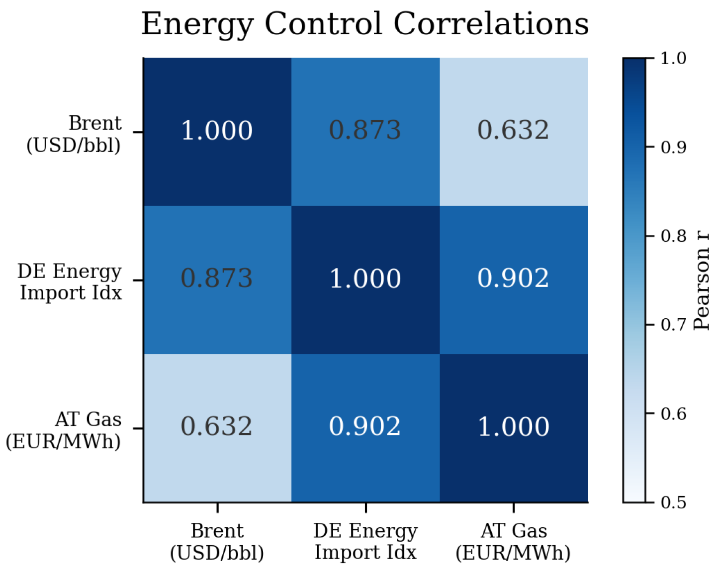
Appendix E.2. Regression Coefficient Plots: Disaggregated Data
The main text reports results for the aggregated duration-weighted monthly panel. The figures in this subsection replicate the key regression outputs using the original, disaggregated offer-spell data. Because each raw spell enters as a separate observation, the estimating environment differs from the aggregated panel, but the qualitative patterns are consistent throughout.
Figure A2 shows the pooled TWFE estimates on the disaggregated data. The left panel is the standard post-payment TWFE; the right panel is the sequential specification. The larger adjustment during the reporting-only phase is visible here as in the aggregated counterpart.
Figure A3 reports category-specific TWFE coefficients on the disaggregated data, ordered by expected SUP exposure. The pooled average masks substantial heterogeneity. Tobacco filters and food containers display positive and comparatively precise estimates; wet wipes, plastic wrap, and non-deposit bottles show negative coefficients. To-go cups, the largest treated category, exhibits only a small negative estimate. Plastic bags has a large positive point estimate but very wide confidence intervals given only four treated units in the raw data.
Figure A4 presents the balloon event study on the disaggregated data. The timing and magnitude of the price response are consistent with the aggregated results reported in Section 5.7 and Table A10: a large, immediate increase at the first payment date that remains elevated for several months before fading.
Figure A2.
Coefficient plots for the pooled TWFE specifications using the original disaggregated offer-spell sample. Left: Standard TWFE with a single post-payment interaction. Right: Sequential multiperiod TWFE () separating the reporting-only and payment-due phases. Points show coefficient estimates; horizontal bars indicate 95% confidence intervals. Significance: * .
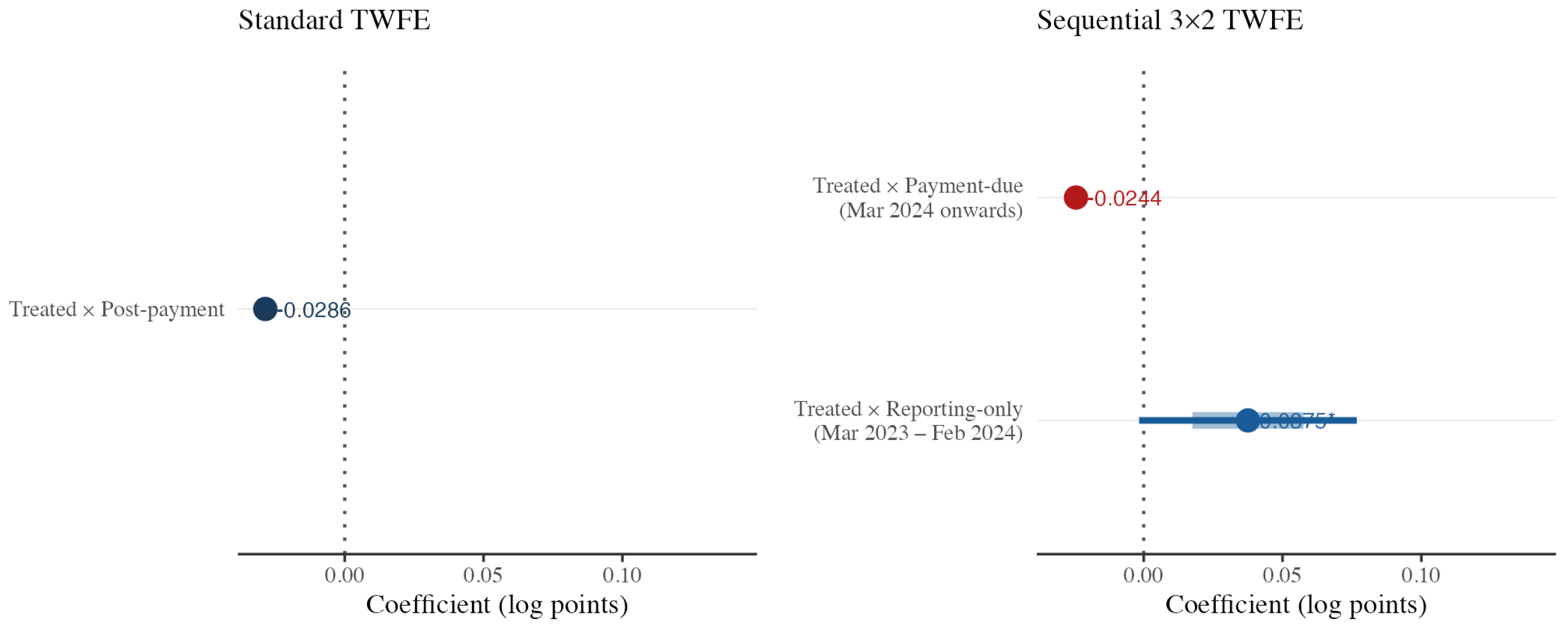
Figure A3.
Category-specific TWFE estimates for the original disaggregated offer-spell sample, ordered by expected SUP exposure. Points show category-level treatment coefficients (log points); horizontal bars indicate 95% confidence intervals. Significance: ** , *** .
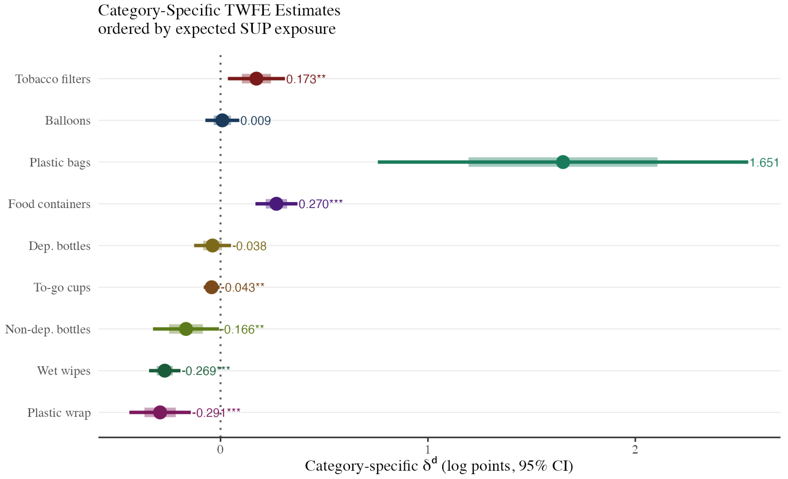
Figure A4.
Event-study coefficients for Austrian balloon prices in the original disaggregated offer-spell data. Points show month-specific coefficient estimates relative to the omitted pre-payment reference period; vertical bars indicate 95% confidence intervals. The vertical dashed line marks the first payment month (March 2024).
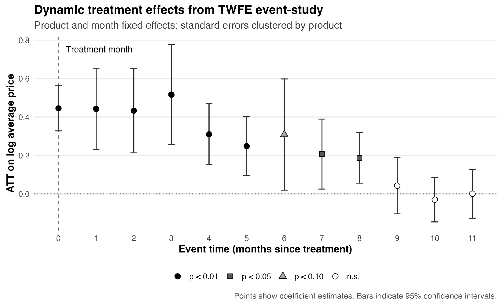
Appendix E.3. Energy Input-Price Series
Figure A5 presents the three energy controls in a grid. The top row covers the full sample (January 2020 to December 2025); the bottom row restricts attention to the estimation event window (March 2023 to March 2025), which brackets treatment onset by twelve months on either side.
All three series peak sharply in 2022, reflecting the European energy crisis following Russia’s invasion of Ukraine in February of that year. The German energy import index reaches approximately 260 (August 2022), Austrian gas prices peak at approximately €216/MWh (September 2022), and Brent crude reaches roughly $122/bbl (June 2022). By reporting onset in March 2023, all three had declined substantially but remained materially above pre-2022 levels, creating the potential for lagged input-cost confounding during the reporting phase. By payment onset in March 2024 energy prices had fallen further; this declining backdrop is, if anything, favorable for identifying the regulatory effect in the payment-due period.
Figure A5.
Energy input-price controls: full sample (top row, 2020–2025) and event window (bottom row, March 2023 to March 2025). Left: Brent crude oil (USD/bbl, FRED). Center: German energy import price index (2021 = 100, Destatis). Right: Austrian natural gas spot price (€/MWh, OEGPI). Vertical dotted line: reporting-phase onset (March 2023). Vertical dashed line: Payment-phase onset (March 2024). Blue shading: Reporting-only period. Red shading: Payment-due period.
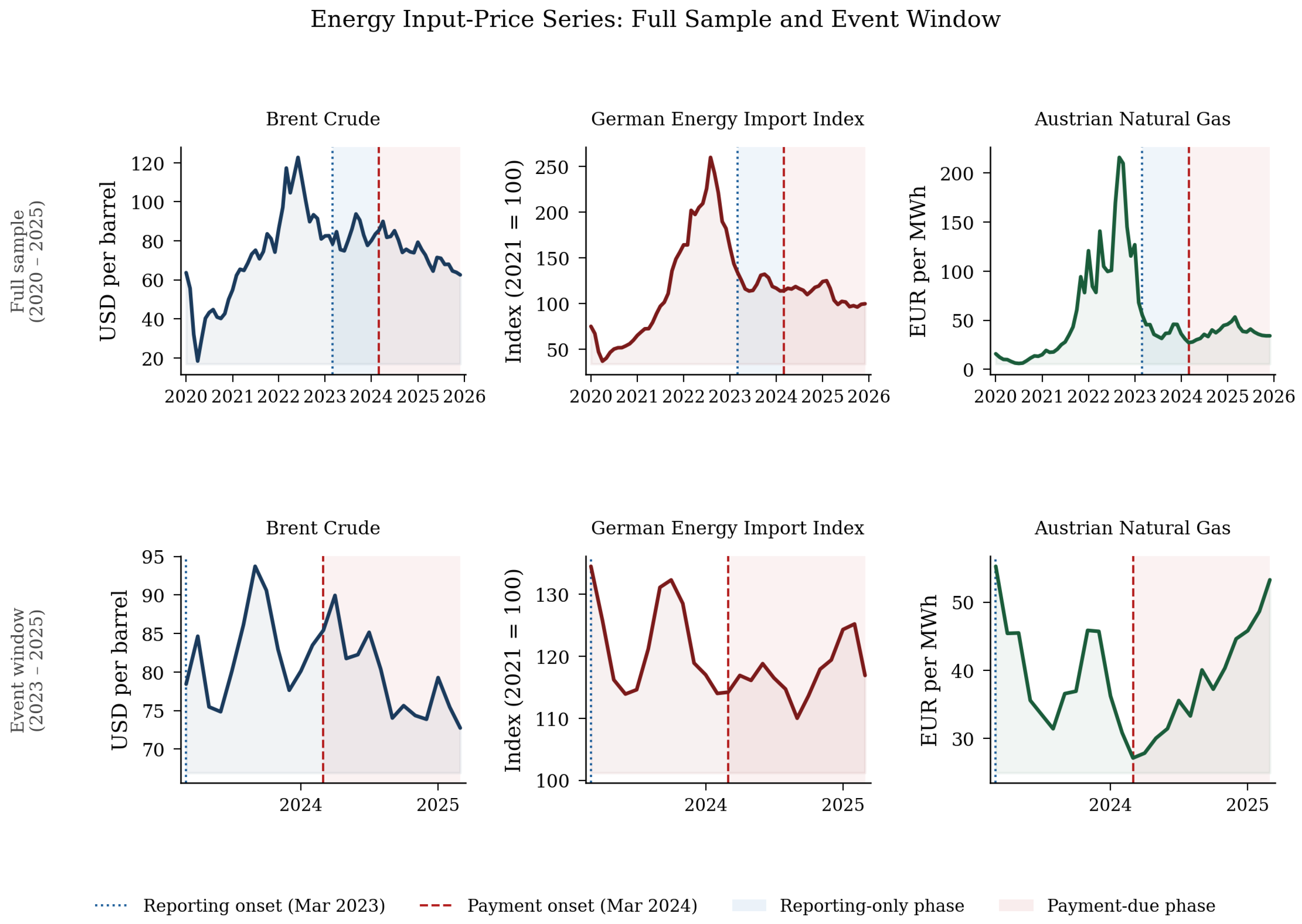
Figure A6 and Figure A7 reproduce the event-window and full-sample panels at a larger scale for ease of inspection, with end-of-window values annotated.
Figure A6.
Energy input-price controls, event window only (March 2023 to March 2025). Left: Brent crude. Center: German energy import index. Right: Austrian gas price. Annotated values indicate the end-of-window observation. Shading and vertical lines follow Figure A5.
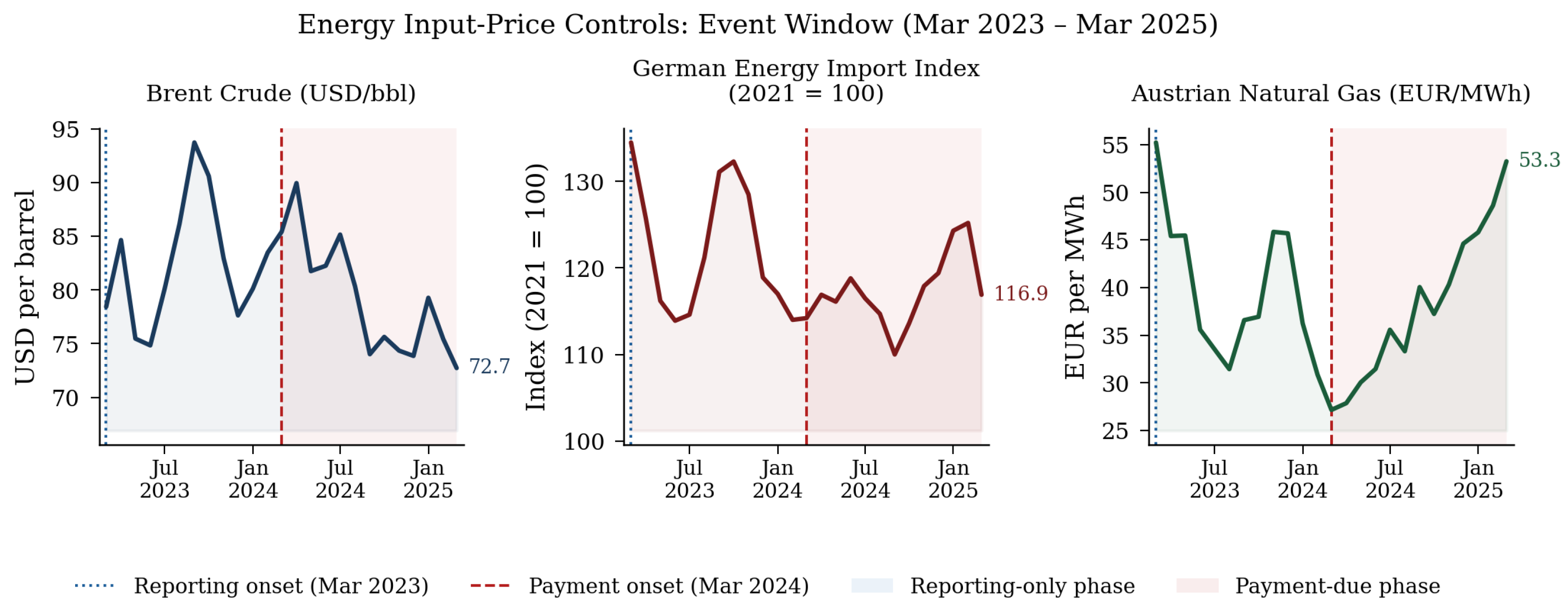
Figure A7.
Energy input-price controls, full sample (January 2020 to December 2025). Left: Brent crude. Center: German energy import index. Right: Austrian gas price. Shading and vertical lines follow Figure A5. The 2022 price spike motivates the inclusion of lagged energy controls in extended specifications.
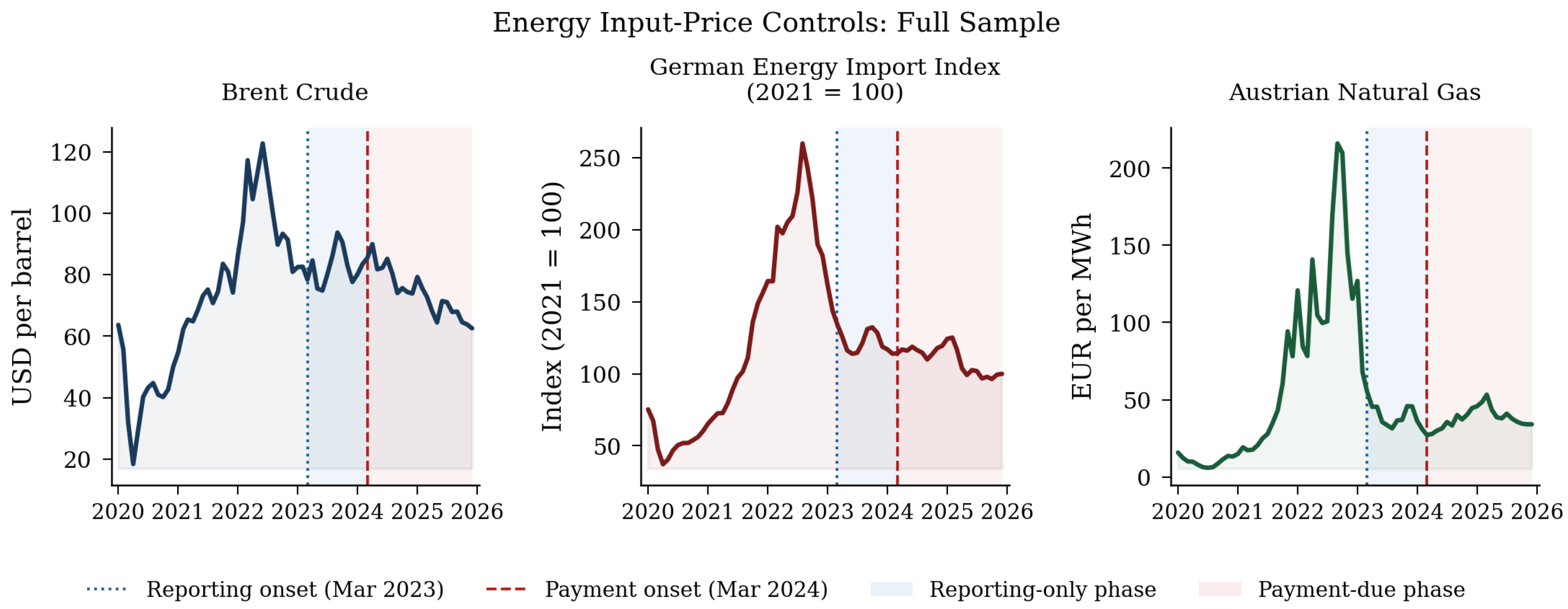
Appendix F. Tables
Appendix F.1. Descriptive Sample Statistics
The treated offer-spell panel is larger than the control panel both in observations and in active units. The treated sample contains 1,738,870 spell-month observations from 20,721 units, while the control sample contains 1,039,833 observations from 7054 units. In levels, mean monthly prices are similar across groups, although the treated sample exhibits substantially greater dispersion. Median prices are somewhat higher among the treated listings than among the controls.
Within the treated sample, exposure is concentrated in a few categories, specifically, to-go cups (15,933 units; 1,312,574 observations). balloons, tobacco filters, wet wipes, and plastic wrap contribute meaningful shares; plastic bags and deposit bottles remain very small. Price levels vary markedly across categories, with the lowest means for wet wipes and plastic wrap and the highest for tobacco filters and plastic bags.
The monthly energy controls vary substantially across the policy phases. Brent crude prices are highest on average during the reporting-only period, while the German energy import index is elevated both before the policy and during the reporting-only phase. Austrian gas prices are most volatile in the pre-policy period (SD = 60.05; maximum above EUR 215/MWh) before stabilizing at lower levels in later phases.
Table A6.
Descriptive statistics: offer-spell panel by treatment status.
Table A7.
Treated sample composition by keyword category.
Table A8.
Descriptive statistics: monthly energy input-price controls by policy phase.
Appendix F.2. Regression Results
Table A9 reports the multiperiod TWFE () estimates under two clustering schemes: unit-level (column 1) and retailer-level (column 2). The point estimates are identical across both columns because clustering affects only the standard errors. Clustering at the retailer level reduces precision sharply for the earlier phase—the report-only coefficient falls below conventional significance thresholds—while the payment-due coefficient remains qualitatively stable. This result, discussed in Section 5.6 of the main text, reflects residual dependence operating partly through seller-wide pricing decisions.
Table A9.
Multiperiod TWFE estimates: sensitivity to clustering level.
Table A10 reports the full set of event-study coefficients for Austrian balloon prices around the first payment date, with Kennedy corrected percentage effects. The month-by-month sequence documents the timing of the price adjustment: a large step at , sustained elevation through , and gradual decay through (December 2024). These coefficients underpin the discussion in Section 5.7 of the main text.
Table A10.
Event-study estimates of Austrian balloon prices around the first payment date.
Appendix G. Notes on Duration-Weighted Panel Analysis
Section 6 of the main text reports four sets of additional analyses using the aggregated duration-weighted panel. The corresponding figures (main text Figure 7, Figure 8, Figure 9, Figure 10, Figure 11, Figure 12, Figure 13, Figure 14 and Figure 15) are not reproduced here. This appendix provides the panel variable reference used across those analyses and brief notes on each subsection.
Table A11 lists the key columns of unit_month_weighted_prices.csv used in Section 6.1, Section 6.2, Section 6.3, Section 6.4 and Section 6.5.
Table A11.
Key columns of unit_month_weighted_prices.csv used in the additional analyses (Section 6.1, Section 6.2, Section 6.3, Section 6.4 and Section 6.5).
- Section 6.1 Category-level heterogeneity and fee-tier test.
The joint model (5) is estimated on category-c treated units against the full control group. Category-specific coefficients and the fee-tier comparison (main text Figure 7, Figure 8 and Figure 9) are discussed fully in the main text. The €450/t tier (balloons, tobacco filters) averages 0.403 log points against for the €225/t group; the tier difference is 0.427 ().
- Section 6.2 Balanced-panel robustness.
The sample is restricted to units observed in at least 25 of the estimation months. The payment-due coefficient rises from 0.394 (unbalanced) to 0.541 (balanced), arguing against compositional exit as the primary driver of the baseline result (main text Figure 10).
- Section 6.3 Seller-type heterogeneity.
The panel is split into marketplace-based sellers (203 treated units) and standalone e-tailers (1850 treated units). The payment-due coefficient is 0.494 for standalone sellers and 0.080 for marketplace sellers, pointing to differences in compliance cost structure or pricing technology (main text Figure 11).
- Section 6.4 Alternative outcome variables and economic magnitude.
Three-period estimates are reported under log price, EUR-level duration-weighted price, and EUR-level unweighted price. The qualitative timing pattern—payment-phase dominant—holds across all three outcomes (main text Figure 12 and Figure 13).
- Section 6.5 Demand-side proxies.
Event-study coefficients for and both rise post-payment, inconsistent with demand contraction. Adding the spell-count control leaves the payment-due price coefficient unchanged (0.397 vs. 0.394), confirming that the estimated effect reflects within-unit repricing (main text Figure 14 and Figure 15).
References
- European Union. Directive (EU) 2019/904 of the European Parliament and of the Council of 5 June 2019 on the reduction of the impact of certain plastic products on the environment. Off. J. Eur. Union 2019, L 155, 1–19. [Google Scholar]
- Fullerton, D.; Metcalf, G.E. Environmental controls, scarcity rents, and pre-existing distortions. J. Public Econ. 2001, 80, 249–267. [Google Scholar] [CrossRef] [Scilit]
- Weyl, E.G.; Fabinger, M. Pass-through as an economic tool: Principles of incidence under imperfect competition. J. Political Econ. 2013, 121, 528–583. [Google Scholar] [CrossRef] [Scilit] [PubMed]
- Marion, J.; Muehlegger, E. Fuel tax incidence and supply conditions. J. Public Econ. 2011, 95, 1202–1212. [Google Scholar] [CrossRef] [Scilit]
- Besley, T.J.; Rosen, H.S. Sales taxes and prices: An empirical analysis. Natl. Tax J. 1999, 52, 157–178. [Google Scholar] [CrossRef] [Scilit]
- Convery, F.; McDonnell, S.; Ferreira, S. The most popular tax in Europe? Lessons from the Irish plastic bags levy. Environ. Resour. Econ. 2007, 38, 1–11. [Google Scholar] [CrossRef] [Scilit]
- Homonoff, T.A. Can small incentives have large effects? The impact of taxes versus bonuses on disposable bag use. Am. Econ. J. Econ. Policy 2018, 10, 177–210. [Google Scholar] [CrossRef] [Scilit]
- Walls, M. Deposit–Refund Systems in Practice and Theory; Resources for the Future: Washington, DC, USA, 2011; pp. Discussion Paper 11–47. [Google Scholar]
- European Parliament and Council. Regulation (EU) 2025/40 of the European Parliament and of the Council of 19 December 2024 on packaging and packaging waste, amending Regulation (EU) 2019/1020 and Directive (EU) 2019/904, and repealing Directive 94/62/EC. Off. J. Eur. Union 2025. Available online: http://data.europa.eu/eli/reg/2025/40/oj (accessed on 18 May 2026).
- Reichel, F. Political Interventions to Reduce Single-Use Plastics (SUPs) and Price Effects: An Event Study for Austria and Germany. arXiv 2025, arXiv:2510.15617v2. [Google Scholar]
- Roth, J.; Sant’Anna, P.H.C.; Bilinski, A.; Poe, J. What’s Trending in Difference-in-Differences? A Synthesis of the Recent Econometrics Literature. J. Econom. 2023, 235, 2218–2244. [Google Scholar] [CrossRef] [Scilit]
- Altstoff Recycling Austria AG. Lizenzierungsservices für Verpackungen. 2026. Available online: https://www.ara.at/ara-lizenzierung-verpackungen (accessed on 14 April 2026).
- Wirtschaftskammer Österreich. Information on the Austrian Packaging Ordinance 2014. 2026. Available online: https://www.wko.at/en/information-on-the-austrian-packaging-ordinance-2014 (accessed on 14 April 2026).
- Umweltbundesamt (UBA). Onlineplattform DIVID des Einwegkunststofffonds Gestartet. 2024. Available online: https://www.umweltbundesamt.de/presse/pressemitteilungen/onlineplattform-divid-des-einwegkunststofffonds (accessed on 14 April 2026).
- Packaging Europe. What Do Rising Commodity Prices Linked with the War in Ukraine Mean for Glass, Metal and Plastic Packaging? 2022. Available online: https://packagingeurope.com/news/what-do-rising-commodity-prices-linked-with-the-war-in-ukraine-mean-for-glass-metal-and-plastic-packaging/8266.article (accessed on 14 April 2026).
- Plastics Europe. The Impact of the Energy Crisis on the European Plastics Manufacturers. 2022. Available online: https://plasticseurope.org/media/the-impact-of-the-energy-crisis-on-the-european-plastics-manufacturers/ (accessed on 14 April 2026).
- Roth, J.; Sant’Anna, P.H.C. When Is Parallel Trends Sensitive to Functional Form? Econometrica 2023, 91, 737–747. [Google Scholar] [CrossRef] [Scilit]
- Callaway, B.; Sant’Anna, P.H.C. Difference-in-differences with multiple time periods. J. Econom. 2021, 225, 200–230. [Google Scholar] [CrossRef] [Scilit]
- Sun, L.; Abraham, S. Estimating dynamic treatment effects in event studies with heterogeneous treatment effects. arXiv 2021, arXiv:1804.05785. [Google Scholar] [CrossRef] [Scilit]
- Bertrand, M.; Duflo, E.; Mullainathan, S. How much should we trust differences-in-differences estimates? Q. J. Econ. 2004, 119, 249–275. [Google Scholar] [CrossRef] [Scilit]
- Cameron, A.C.; Gelbach, J.B.; Miller, D.L. Robust inference with multiway clustering. J. Bus. Econ. Stat. 2011, 29, 238–249. [Google Scholar] [CrossRef] [Scilit]
- Hackl, F.; Kummer, M.E.; Winter-Ebmer, R.; Zulehner, C. Market Structure and Market Performance in E-Commerce. Eur. Econ. Rev. 2014, 68, 199–218. [Google Scholar] [CrossRef] [Scilit]
- Roth, J. Pretest with Caution: Event-Study Estimates after Testing for Parallel Trends. Am. Econ. Rev. Insights 2022, 4, 305–322. [Google Scholar] [CrossRef] [Scilit]
- Rambachan, A.; Roth, J. A More Credible Approach to Parallel Trends. Rev. Econ. Stud. 2023, 90, 2555–2591. [Google Scholar] [CrossRef] [Scilit]
- CNBC. Hormuz Blockade Could Deepen World’s Worst Energy Crisis—And Risk a Dangerous Misstep; CNBC: Englewood Cliffs, NJ, USA, 2026; Available online: https://www.cnbc.com/ (accessed on 14 April 2026).
- Packaging Gateway. Oil Shock Sends Packaging Costs Soaring; Packaging Gateway: London, UK, 2026; Available online: https://www.packaging-gateway.com/ (accessed on 14 April 2026).
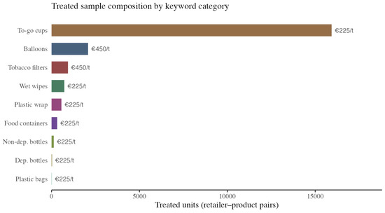
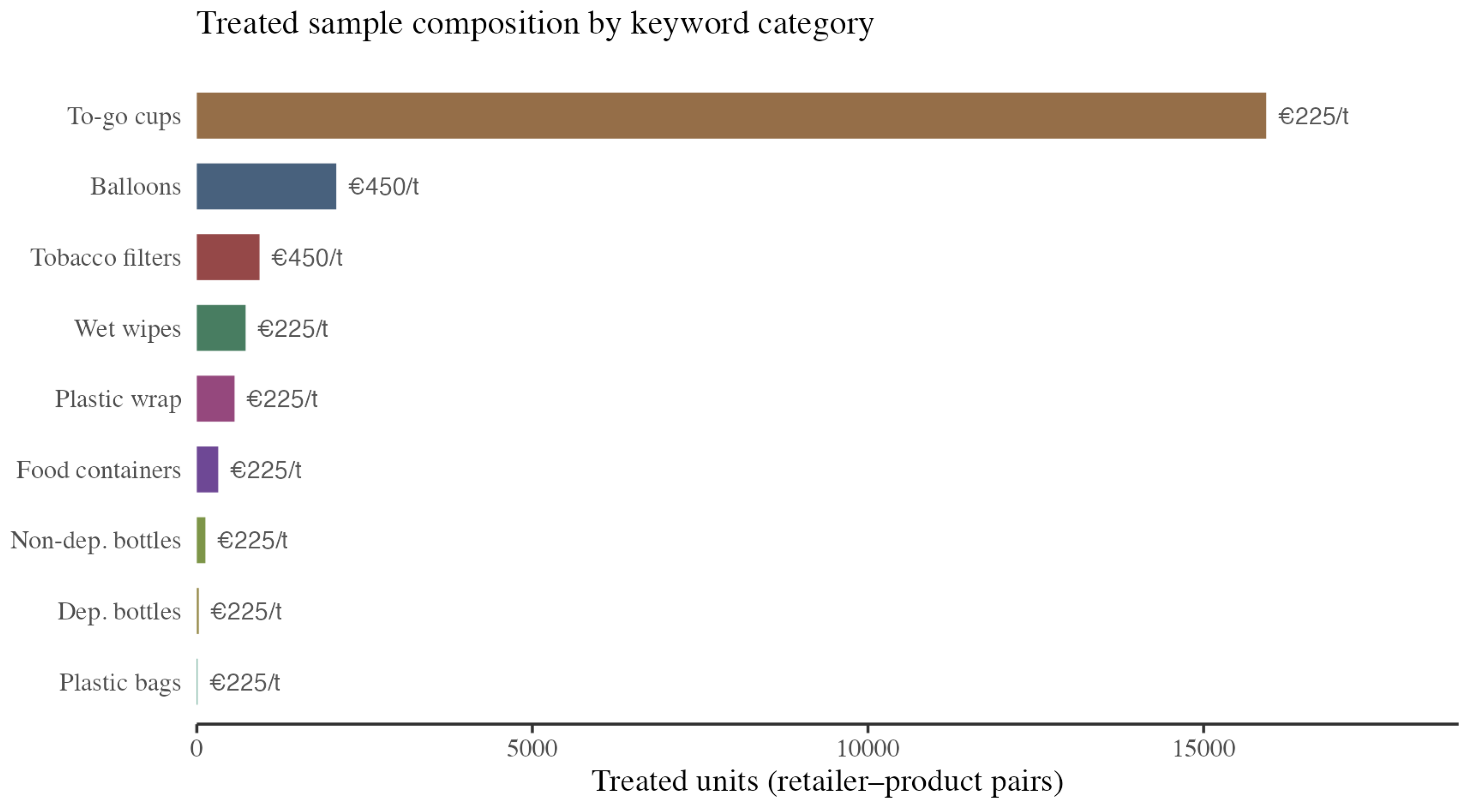
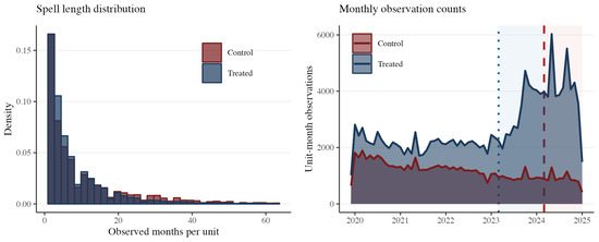
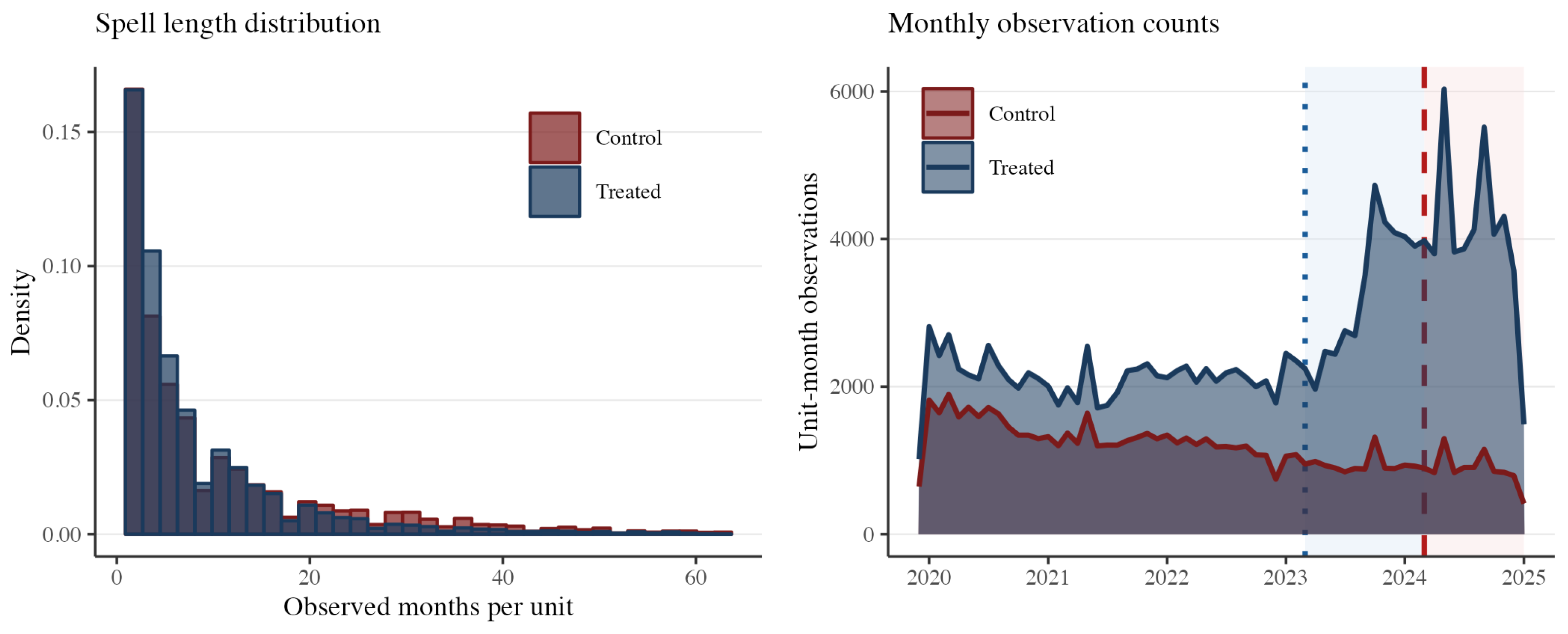
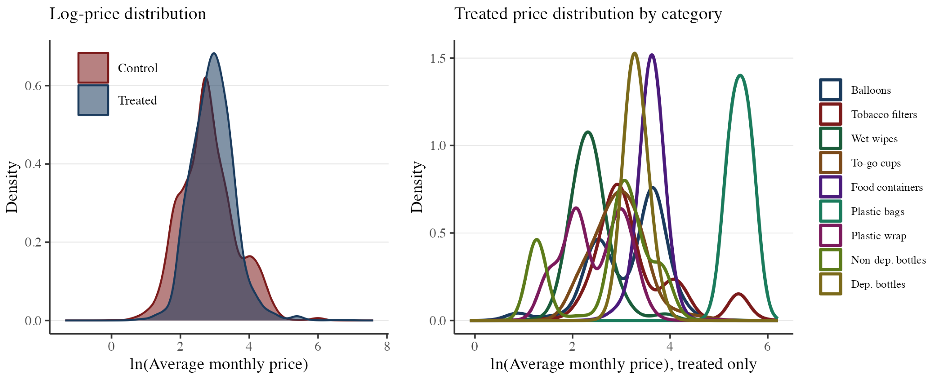
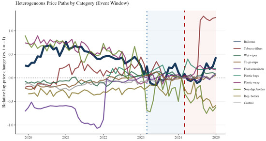
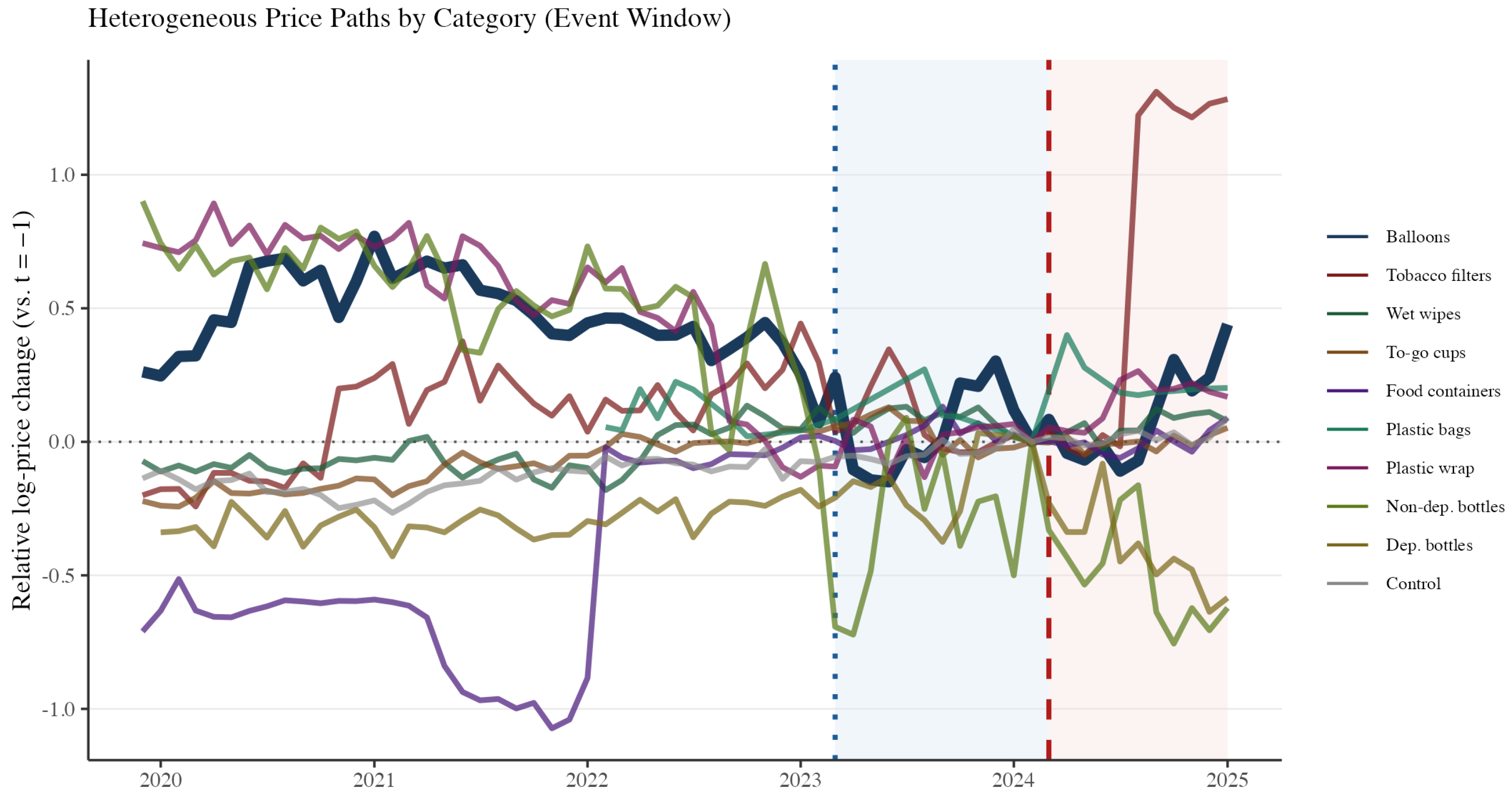
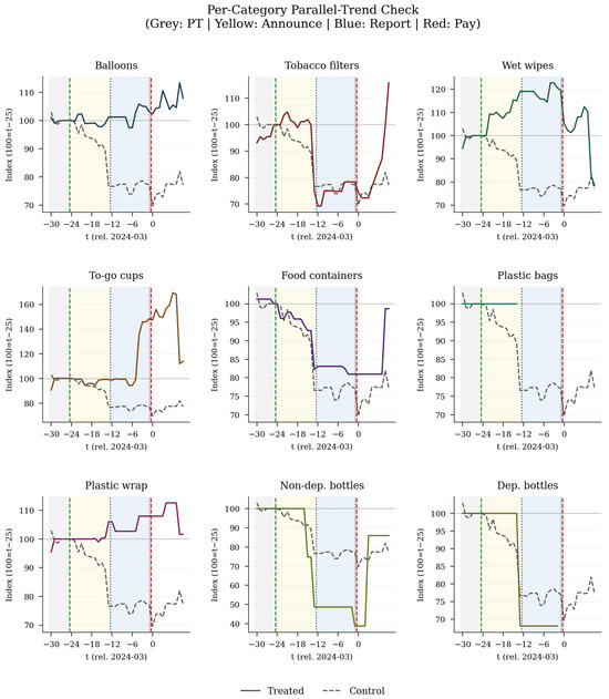
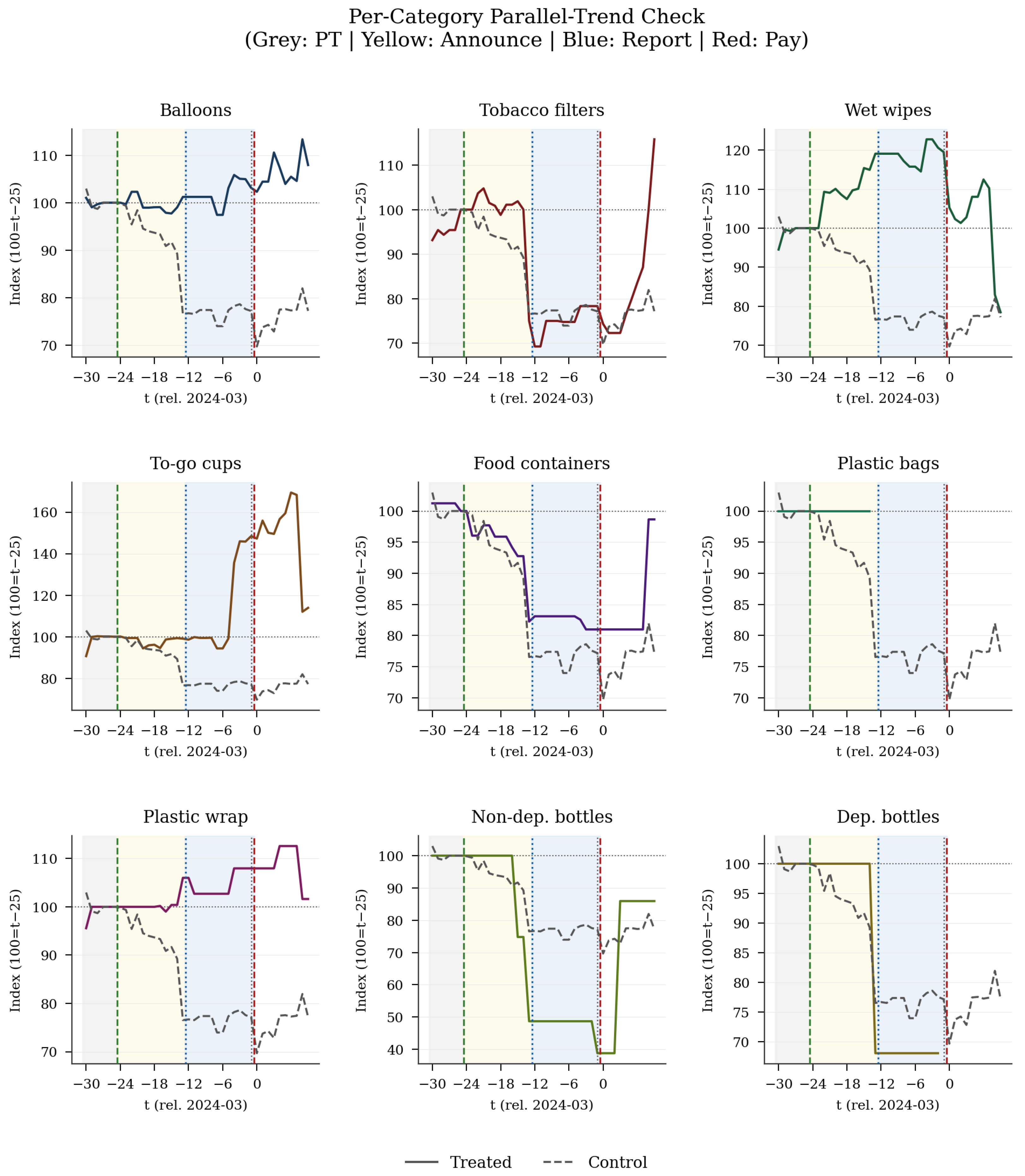
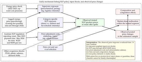
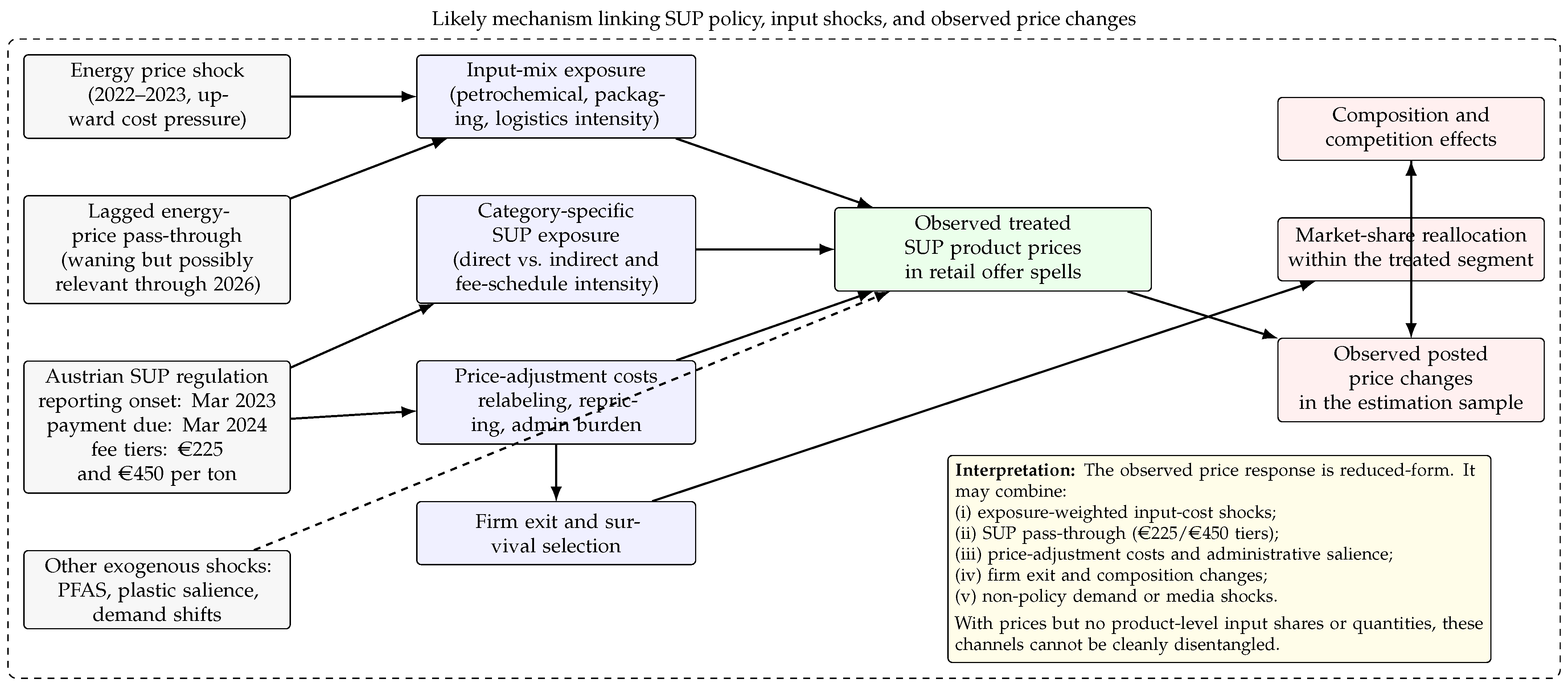
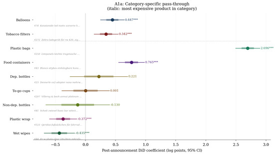
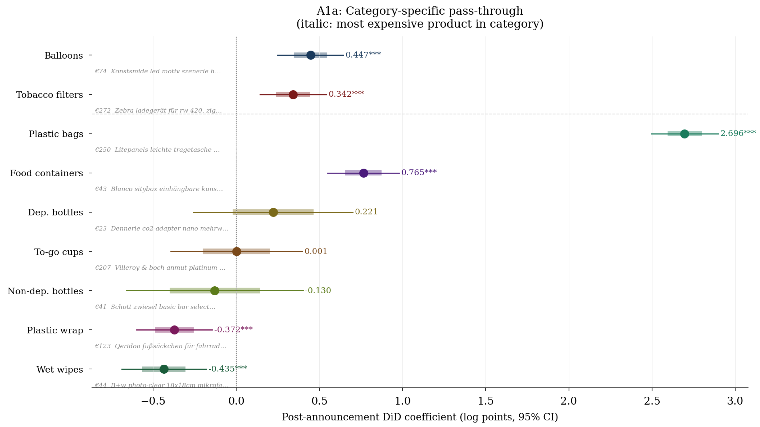
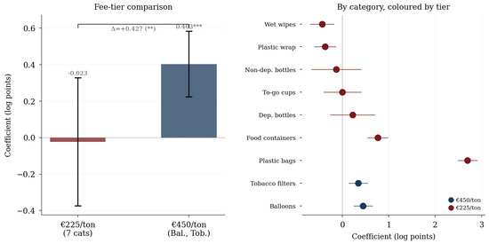
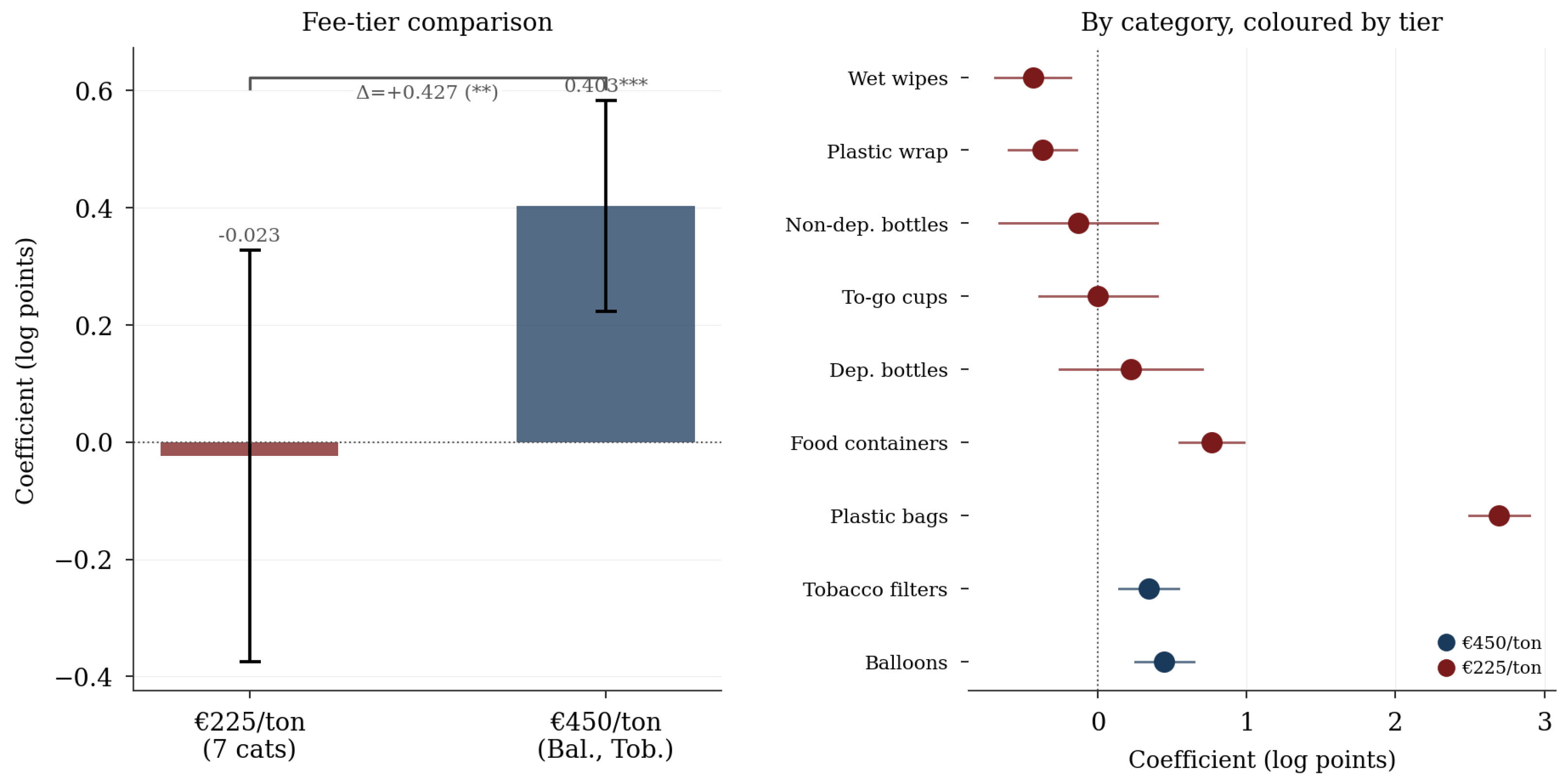
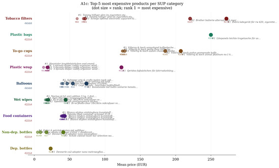
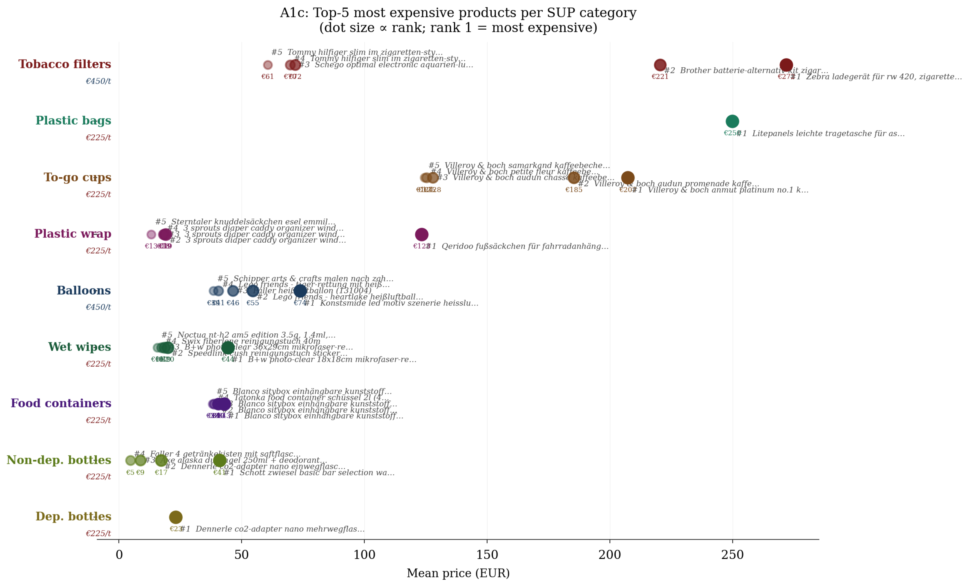
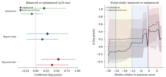
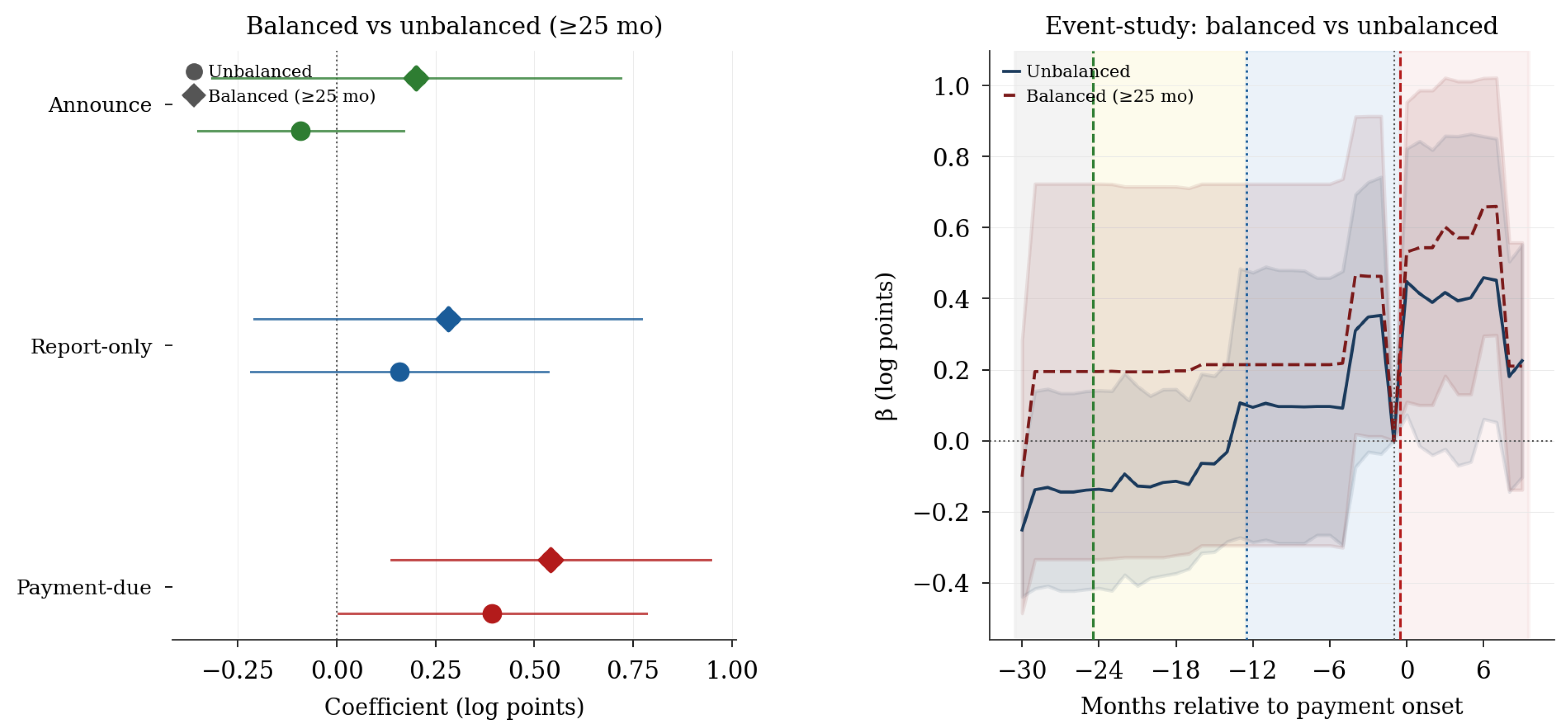
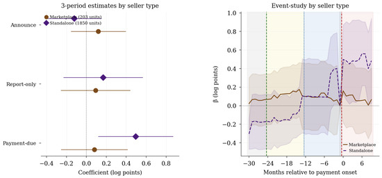
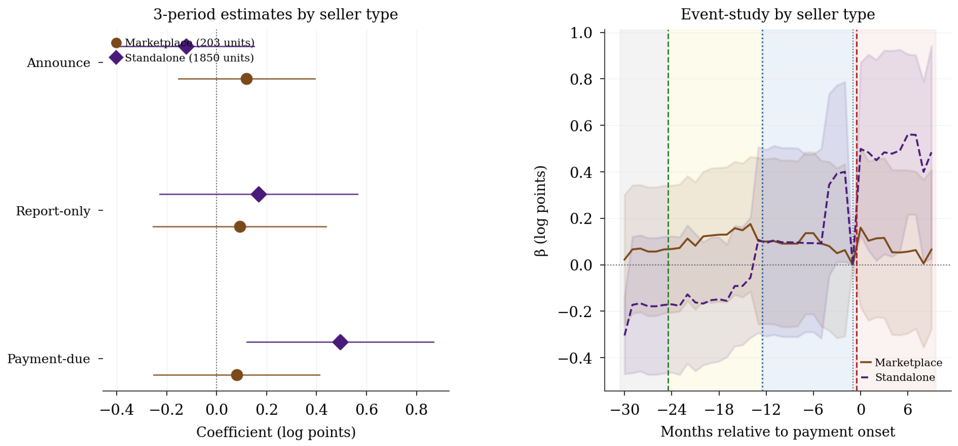
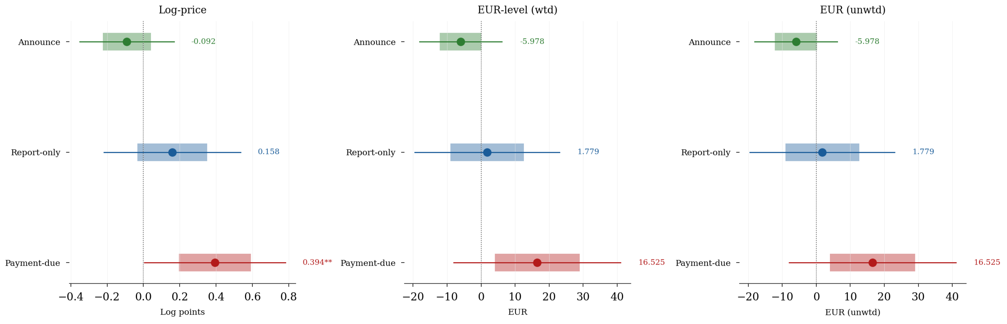
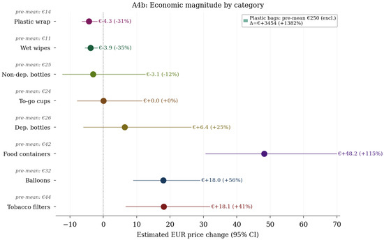
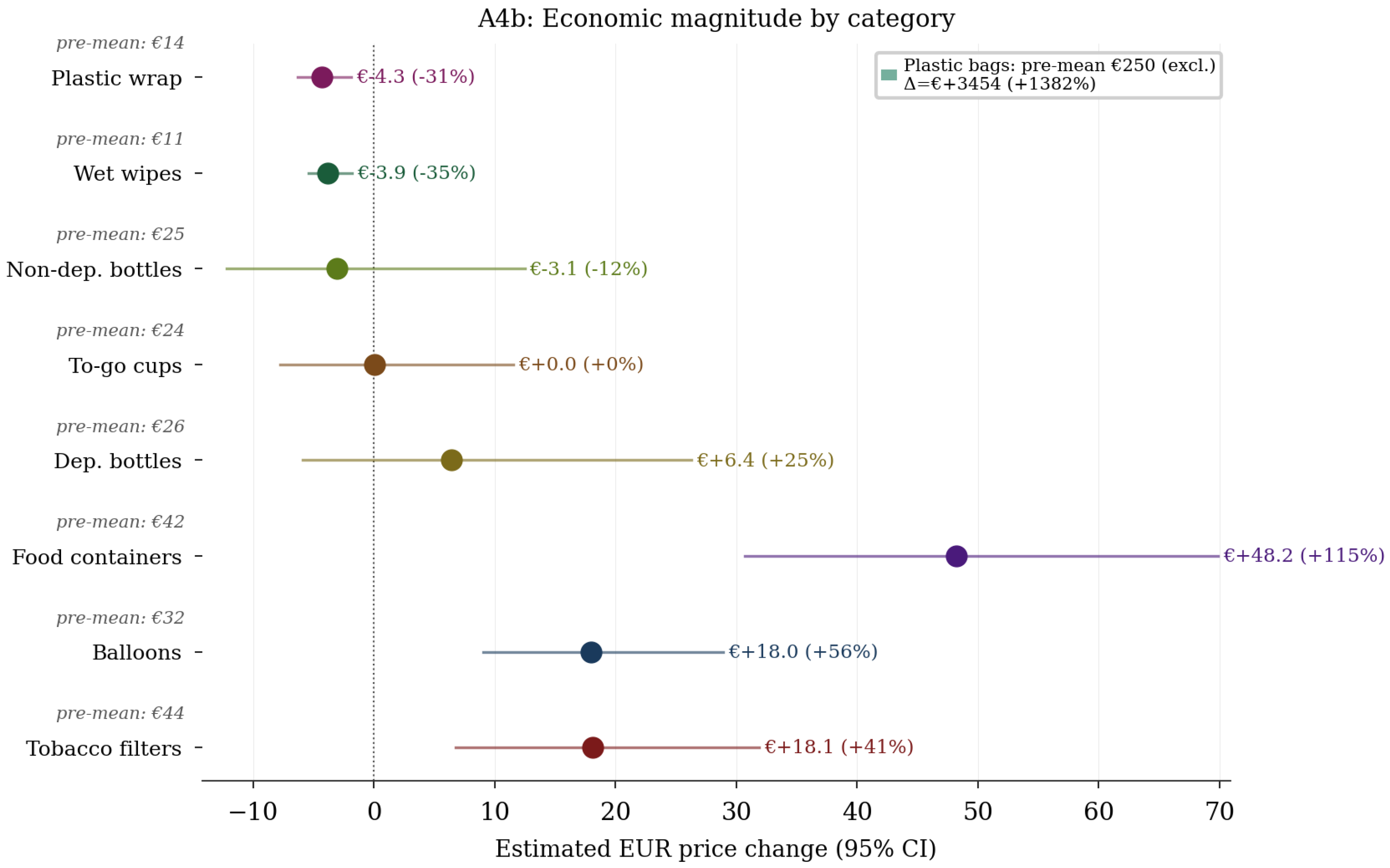
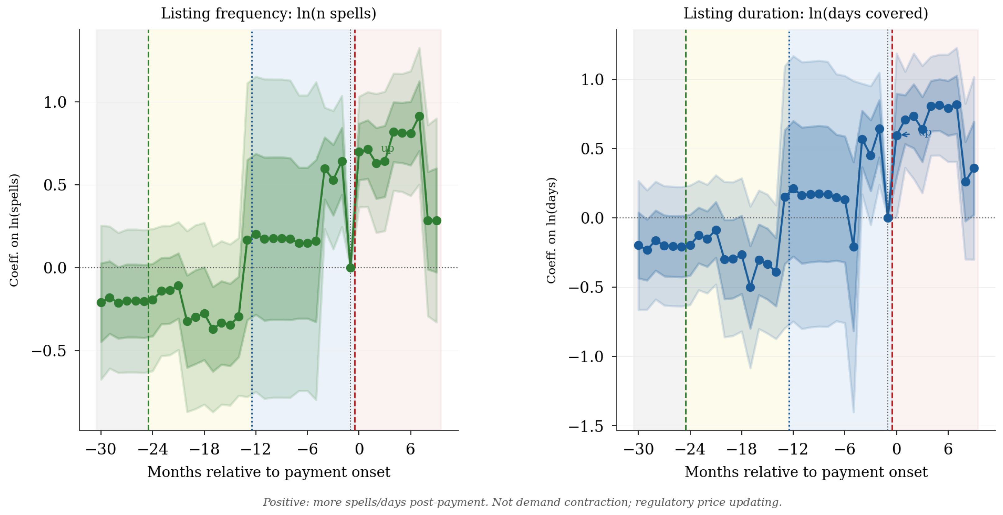
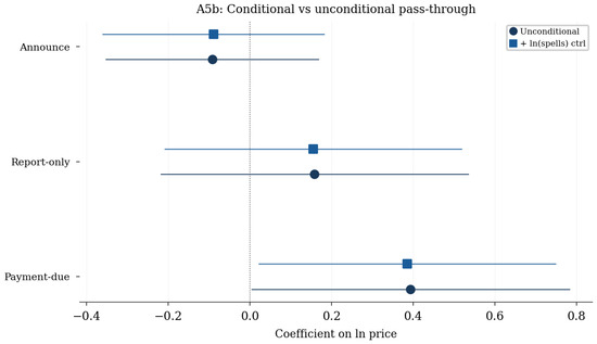
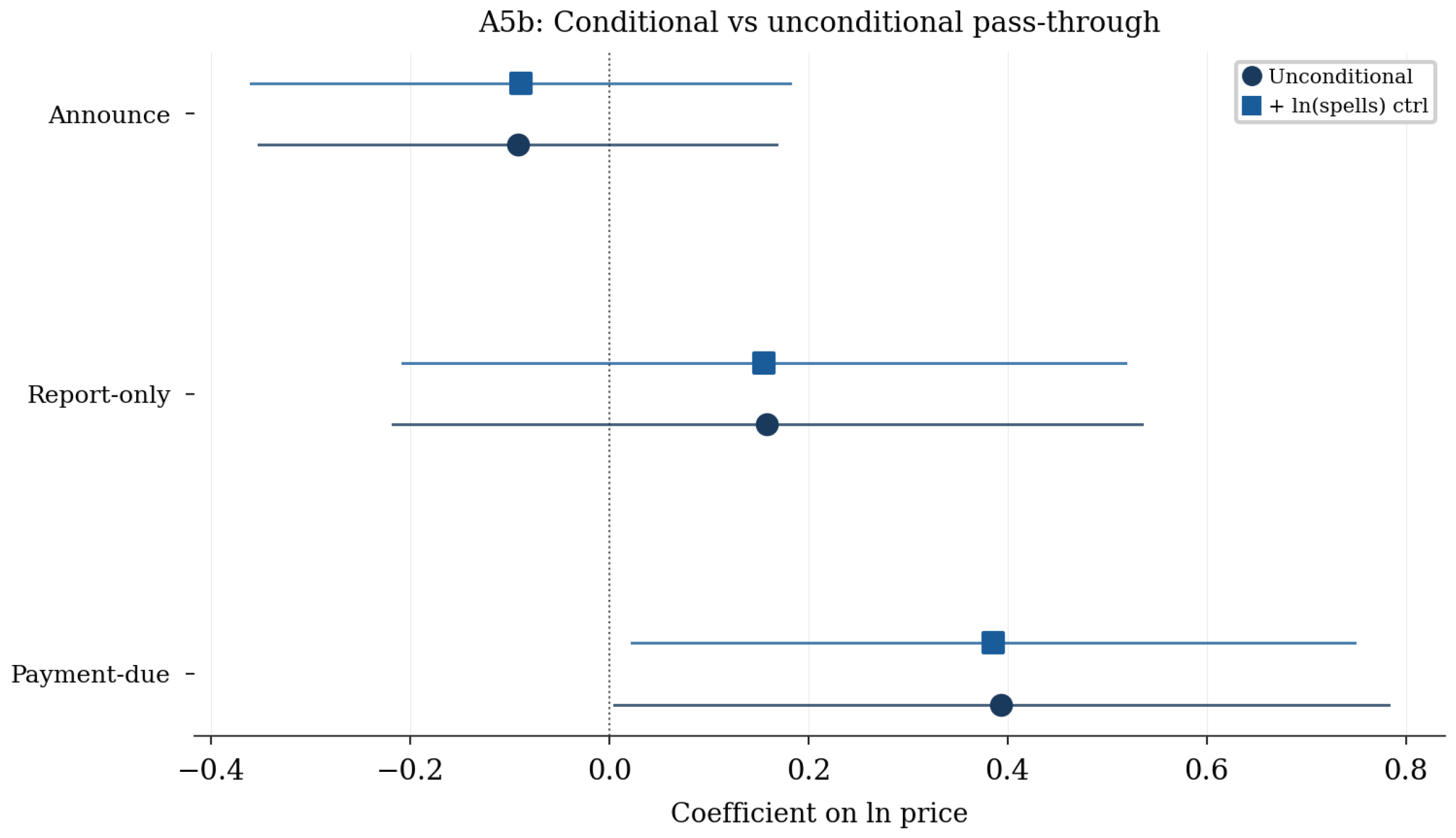

Disclaimer/Publisher’s Note: The statements, opinions and data contained in all publications are solely those of the individual author(s) and contributor(s) and not of MDPI and/or the editor(s). MDPI and/or the editor(s) disclaim responsibility for any injury to people or property resulting from any ideas, methods, instructions or products referred to in the content. |
© 2026 by the author. Licensee MDPI, Basel, Switzerland. This article is an open access article distributed under the terms and conditions of the Creative Commons Attribution (CC BY) license.