Central Conics in ${\mathbb{H}}^2$ Are Fibers over the Group of Steiner Conics

Abstract

We provide an intrinsic construction of the central conics in the real hyperbolic plane ${\mathbb{H}}^2$, whereby each conic C is the composition of a unique pair of Steiner conics (those generated by collineations). The composition is achieved by elliptic curve addition on intersection points of the two components with their orthogonal trajectories, which have a natural representation as genus 1 curves in any inversive model of ${\mathbb{H}}^2$. The central Steiner conics that have a focal axis L are identified with the subgroup $G\left(L\right)$ of collineations generated by reflections in the lines perpendicular to L. We obtain a $G\left(L\right)$-equivariant partition of the central conics by defining the fiber over $g\in G\left(L\right)$ to be the set of compositions C such that $\pi \left(C\right)=g$. Here, $\pi \left(C\right)$ is the unique Steiner conic tangent to C at the points on L, and is the product of the two elements in $G\left(L\right)$ that represent the components of C. We use the terminology of fibers strictly in an incidence-geometric sense.

1. Introduction

There currently appears to be no fundamentally intrinsic construction of conics in the real hyperbolic plane ${\mathbb{H}}^2$. Such a construction would not treat ${\mathbb{H}}^2$ as a sub-geometry of an ambient space, such as a projective space, but would require only the incidence properties of the plane and the action of the collineation group. One reason this has not been achieved may be that the subject is often relegated to ‘classical’ geometry, with no urgency to revisit it from the viewpoint of modern incidence geometry. In this article we provide an intrinsic construction by viewing ${\mathbb{H}}^2$ as a linear incidence geometry, where two distinct points are on exactly one line and two distinct lines meet in at most one point, using conformal models to represent figures and verify claims analytically.

A first step toward such a construction was taken in [1]. There, we classified the Steiner conics in ${\mathbb{H}}^2$, defining them, as follows, as a generalization of Jakob Steiner’s construction in [2] (pp. 134–140).

Definition 1.

Let T be a collineation of a planar incidence geometry. The Steiner conic $E\left(T;P\right)$ afforded by T at point P is the locus of intersections $L\cap T\left(L\right)$ for the lines L concurrent at P. The conic $E\left(T_1;P_1\right)$ is congruent to $E\left(T;P\right)$ if, for some collineation $T_0$, $T_1=T_{0}T{T}_0^{-1}$ and $P_1=T_0\left(P\right)$. If the geometry is oriented, $E\left(T;P\right)$ is direct if T preserves orientation, and opposite if T reverses orientation. The conic is degenerate if $T\left(P\right)=P$ or if $T\left(L\right)=L$ for some L.

It is possible for all conics in a planar geometry, defined algebraically or by other means, to be Steiner conics. This is the case in a projective plane over a field, as discussed in [3] (p. 80). From this viewpoint, the “conic sections”—ellipses, parabolas, and hyperbolas—are classified by the invariants of affine collineations that afford them. By contrast, the collineation group of ${\mathbb{H}}^2$ consists entirely of isometries if a metric is imposed. This constrains the Steiner conics to the $E\left(T;P\right)$ in [1] where we showed them to be proper subsets of seven of the eleven categories of curves described in the classical sources [4,5]. Those categories extended work by Enrico D’Ovidio and others in the 1890s. They were described, non-intrinsically, by intersecting cones with a hyperbolic domain (analogous to the conic sections of Apollonius). The numbering and descriptors for these categories in [5] (p. 119), which correspond to the figures in [4] (p. 229), are reprised in Section 2 for the central conics, characterized by having two perpendicular lines of symmetry.

The central conics are the subject of our discussion because our principal results require these two lines of symmetry, the axes of the conics. As such, $E\left(T;P\right)$ will always denote a central Steiner conic, and C will always designate a central conic in ${\mathbb{H}}^2$. We write $\mathcal{D}$ for the set of direct $E\left(T;P\right)$ and $\mathcal{O}$ for the set of opposite $E\left(T;P\right)$. The set ${\mathcal{D}}_0$ consists of the members of $\mathcal{D}$ with no absolute points on the boundary of ${\mathbb{H}}^2$. Upon choosing a set of congruence representatives ${\mathcal{D}}_0$, we use elliptic curve addition on their orthogonal trajectories to define the composition C of any two members of ${\mathcal{D}}_0$. This is our main result, which we state in Section 2. Apart from references to [1] for clarification purposes, our aim is to keep this presentation as self-contained as possible and of interest to the pedagogical community. The following outline provides context for the proof of our Main Theorem and its consequences in later sections.

In Section 3 we use the hyperboloid model of ${\mathbb{H}}^2$ to construct a family of elliptic space curves and describe the addition on their points. In Section 4 we represent points as complex numbers by projecting them into the conformal disk $\mathbb{D}$, where it is easy to visualize these curves and those in ${\mathcal{D}}_0$ as an orthogonal system. That the composition of a member of ${\mathcal{D}}_0$ with itself is a circle is proved in Section 5, followed by a formula in $\mathbb{D}$ for the elliptic curve addition. In Section 6 we derive some algebraic identities required for the proof, in Section 7, of the Main Theorem. In Section 8 the remaining categories of central conics listed in Section 2 will be produced from the compositions C. In Section 9 we use the Main Theorem and an intrinsic involution on the half-planes of ${\mathbb{H}}^2$ that interchanges ${\mathcal{D}}_0$ and $\mathcal{O}$ to describe a group structure on ${\mathcal{D}}_0\cup \mathcal{O}$. We define the fiber over each member of this group in Section 10 and partition the central conics into fibers. When representing a group G, the set of pairs in $G\times G$ that contract under multiplication to a given member of G is a useful construction (for example, in the description of fibers for principal bundles over orthogonal groups). The fiber structure we develop can be viewed as a geometric interpretation of this construction for $G={\mathcal{D}}_0\cup \mathcal{O}$. The reader will note from the discussion of group structure in Section 9 that G is isomorphic to a split orthogonal group. However, our fibration is algebraic and does not involve topology.

For brevity throughout, we omit the details of routine calculations unless they are essential to the argument at hand. Several of these calculations are characteristically intricate. They have been performed manually and then thoroughly checked with the MuPAD CAS. Details of two lengthy calculations can be found in Appendix A.

Note. The implementation of elliptic curve addition on orthogonal trajectories of the ellipses is motivated by the following observation: In any inversive model of ${\mathbb{H}}^2$, such as the Poincaré disk or the upper-half plane, genus 1 curves are part of the analytic landscape. However, fundamental connections between them and incidence geometry seem to be absent from the literature, an irony of history since Jacobi and other developers of elliptic curve theory were Jakob Steiner’s colleagues, and Steiner himself proved many synthetic theorems about cubics and quartics. We believe their properties should receive more attention in this context (see Remark 1 in Section 4).

2. Background and Statement of Main Theorem

Before stating our main result we establish some basic terminology by way of a brief summary of the classification of the $E\left(T;P\right)$. We note that some terms have been adapted to this discussion and differ slightly from those in [1]. First, it is convenient to describe the translation component of the collineation T in terms of distance, whereby the eccentricity $ϵ$ of $E\left(T;P\right)$ is a function of the distance s between P and $T\left(P\right)$. If $E\left(T;P\right)\in \mathcal{D}$ then $ϵ=\sinh s$. We write $E_{ϵ}$ for the Steiner conic in this case and will work with a set of congruence representatives parameterized by $ϵ$. These representatives have common axes of symmetry, hence a common center O. We reserve the term ellipse for an $E_{ϵ}$ with $0\le ϵ<1$, where $E_0$ is the degenerate ellipse O. The ellipses comprise the subset ${\mathcal{D}}_0$. Each ellipse is a special case of a locus $C\left(\kappa ,\eta \right)$ consisting of points the sum of whose distances from two foci is $\kappa$, where $\eta$ is the distance between the foci; for an ellipse, $ϵ=\tanh \kappa$ and $\tanh \eta ={\tanh }^2\kappa$. The center of $C\left(\kappa ,\eta \right)$ is the midpoint of the segment between the foci. Further, the focal axis of $C\left(\kappa ,\eta \right)$ is the line through the foci, and the transverse axis of $C\left(\kappa ,\eta \right)$ is the line perpendicular to the focal axis at the center. If $ϵ>1$ we call $E_{ϵ}$ a hyper-ellipse. The conic $E_1$ is the pair of equidistant curves with angle-of-parallelism ${\displaystyle \frac{\pi }{4}}$ relative to the focal axis of the ellipses. The members of $\mathcal{O}$ are all central; we refer to them as hyperbolas and provide parameters for them in Section 9.

The seminal objects for this discussion are the ellipses. We recall from [1] their essential properties that will be used later. First, the open region $\mathcal{E}$ bounded by $E_1$ (not introduced explicitly in [1]) is the disjoint union of the ellipses $E_{ϵ}$. From equation 5.2 in [1] (p. 139), the representation of $E_{ϵ}$ in the conformal disk $\mathbb{D}$ is given by the polar equation

$$r^4-2r^2\left(\cos 2\varphi +{\displaystyle \frac{2}{{ϵ}^2}}\right)+1=0$$

if $ϵ\ne 0$. Note that this equation is also satisfied by ${\displaystyle \frac{1}{r}}$, that is, the polar representation includes the inversion of $E_{ϵ}$ in the unit circle; these are points of the algebraic curve not in ${\mathbb{H}}^2$. This observation will be relevant in Section 4 when we derive a complex number formula in $\mathbb{D}$ for addition on the orthogonal trajectories of the $E_{ϵ}$. Let $ϵ=\tanh \kappa$. Then the points of the ellipse on its focal axis are $\pm i\tanh {\displaystyle \frac{\kappa }{2}}$. The orthogonal trajectories of the ellipses, which we require for the Main Theorem, were not discussed in [1]. We derive their polar representations in Section 4.

It will suffice to state the Main Theorem in terms of the ellipses, because all of the $E\left(T;P\right)$ are related to them by the process of split inversion. Split inversion is a conformal, incidence-preserving involution on the open half-spaces of a hyperbolic space that interchanges complementary angles-of-parallelism. (The term is not standard but varies with context. See [6], where it is used without an explicit name.) In ${\mathbb{H}}^2$, we have the following definition.

Definition 2.

Let $\mathcal{P}$ be an open half-plane for a given line L in ${\mathbb{H}}^2$. For any $P\in \mathcal{P}$, let $L_P$ be the perpendicular to L through P. The split inversion of P in L is the point $P^{‡}\in L_P\cap \mathcal{P}$ such that the angle-of-parallelism to L at $P^{‡}$ is the complement of the angle-of-parallelism to L at P.

This definition is simple and elegant but working in terms of angles-of-parallelism would complicate our constructions unnecessarily. Instead, we note that split inversion can be implemented by inversion in the pair of equidistant curves for L whose angles with the boundary of the plane are ${\displaystyle \frac{\pi }{4}}$. For example, if L is the focal axis of the ellipse $E_{ϵ}$ then this pair is $E_1$. In Section 4 we will start working within $\mathbb{D}$, representing points as complex numbers. As was shown in [1], split inversion in the focal axis L is given by the formula

$$P\mapsto {\displaystyle \frac{1\pm P^{*}}{P^{*}\mp 1}}$$

where $P^{*}$ is the complex conjugate of P and the signs are determined by the half-plane containing P. Similarly, the split-inversion of P in the transverse axis $L^{\prime }$ is

$$P\mapsto {\displaystyle \frac{1\pm i{P}^{*}}{P^{*}\pm i}}.$$

These formulas were used in [1] to show that if $ϵ\ne 0$ then split-inversion in L interchanges the ellipse $E_{ϵ}$ and the hyper-ellipse $E_{{\displaystyle \frac{1}{ϵ}}}$. (Though the split inversion of $E_0$ is not strictly defined, the pair of points on the boundary that would result will be used in Section 9 to describe reflection in $L^{\prime }$ as a group element.) Split inversion of figures will be obtained from these formulas but we will usually omit the details of calculations.

Our goal is to present an intrinsic construction within the framework of incidence geometry. For context we recall that the central conics depicted in references [4,5] comprise five of the categories in these sources, where they are designated as follows:

C1 Convex hyperbolas.

C2 Concave hyperbolas.

C4 Ellipses.

C9 Equidistant curves.

C10 Proper circles.

Since they fit our definition, we will include two other categories, afforded by degenerate cones:

C9A Pairs of intersecting lines.

C9B Pairs of ultra-parallel lines.

Except for C9, C9A and C9B, these conics are represented in any inversive model of ${\mathbb{H}}^2$ by irreducible algebraic curves. We will see that the $C\left(\kappa ,\eta \right)$ account for C4 and C10. Split inversion of the $C\left(\kappa ,\eta \right)$ in their focal axes will account for C2, and split inversion of the $C\left(\kappa ,\eta \right)$ in their transverse axes for C1. Our construction will also produce the reducible curves C9, C9A and C9B.

The essential fact (see Section 4) is that the $E_{ϵ}$ are orthogonal in ${\mathbb{H}}^2$ to curves $F_{\alpha }$ defined by the following locus condition:

Let O be a designated point on a given line $L^{\prime }$ in ${\mathbb{H}}^2$. For $\alpha \in \left(-{\displaystyle \frac{\pi }{2}},0\right)\cup \left(0,{\displaystyle \frac{\pi }{2}}\right)$, let $F_{\alpha }$ be the locus of points P such that $\measuredangle OPA=\alpha$, where A is the foot of the perpendicular to $L^{\prime }$ from P.

Each $F_{\alpha }$ is symmetric about O. Reflection in $L^{\prime }$ reverses the orientation of $\angle OPA$, interchanging $F_{\alpha }$ and $F_{-\alpha }$. Our representatives for the $E_{ϵ}$ are the $E\left(T;P\right)$ for which O is the midpoint on $L^{\prime }$ of P and $T\left(P\right)$. For any $ϵ>0$, $L^{\prime }$ is considered to be the transverse axis of $E_{ϵ}$, and the line L through O perpendicular to $L^{\prime }$ is its focal axis. Each $F_{\alpha }$ meets $E_{ϵ}$ at two points in ${\mathbb{H}}^2$, one in each half-plane of the focal axis. The $F_{\alpha }$ are invariant under split inversion in L. We will see in Section 3 that the $F_{\alpha }$ have a natural representation on the Minkowski hyperboloid. Using this model (and later its projection into the disk $\mathbb{D}$) we will derive the elliptic curve addition $P_1{\oplus }_{\alpha }{P}_2$ on the points of the algebraic curve containing $F_{\alpha }$. Our main result, the construction of conics in categories C4 and C10, is as follows:

Theorem 1.

Given ellipses $E_{{ϵ}_1}$ and $E_{{ϵ}_2}$ with $0\le {ϵ}_1\le {ϵ}_2$, let $P_1$ and $P_2$ be respective intersections with a given $F_{\alpha }$. Let $\iota =1$ if $P_1$ and $P_2$ are chosen in the same half-plane of the focal axis L and let $\iota =-1$ if they are chosen in opposite half-planes of L. Then, with ${ϵ}_1=\tanh {\kappa }_1$ and ${ϵ}_2=\tanh {\kappa }_2$, the set of points $\left\{P_1{\oplus }_{\alpha }{P}_2\mid \alpha \in \left(-{\displaystyle \frac{\pi }{2}},0\right)\cup \left(0,{\displaystyle \frac{\pi }{2}}\right)\right\}$ for a consistent choice of ι is the locus $C_{\iota }\left(\kappa ,\eta \right)$ where $\kappa ={\kappa }_2+\iota {\kappa }_1$ and $\eta ={\eta }_2-{\eta }_1$.

We refer to $C_{\iota }\left(\kappa ,\eta \right)$ as the composition of $E_{{ϵ}_1}$ and $E_{{ϵ}_2}$ for the value $\iota$, denoting it as convenient by $E_{{ϵ}_1}{\circ }_{\iota }{E}_{{ϵ}_2}$. The intersections of $C_{\iota }\left(\kappa ,\eta \right)$ with L and $L^{\prime }$ are obtained as limiting cases for $\alpha$. Note in particular that if ${ϵ}_1=0$ then $C_{\iota }\left(\kappa ,\eta \right)=E_{{ϵ}_2}$. Also, if ${ϵ}_1={ϵ}_2$ then $\eta =0$, that is, the composition of an ellipse with itself is a circle ($E_0$ if $\iota =-1$); we will prove this special case in advance of the general proof of the theorem. Note that $\tanh \eta =\tanh \left({\kappa }_2+{\kappa }_1\right)\tanh \left({\kappa }_2-{\kappa }_1\right)$, from which it will follow as a corollary to the theorem that $C_{\iota }\left(\kappa ,\eta \right)$ is the composition of a unique pair of ellipses.

As indicated above, several detailed calculations are involved in proof of the Main Theorem 1 that require numerous related variables.

Table 1. Notation.

Geometric Symbol	Definition	Context
$ϵ$, ${ϵ}_j$	Eccentricity	Steiner conic $E\left(T;P\right)$
$\iota$ (Section 2)	$\pm 1$	Position of points relative to focal axis
$\kappa$	Sum of distances to foci	Locus parameter for $C_{\iota }\left(\kappa ,\eta \right)$
$\eta$	Distance between foci	Locus parameter for $C_{\iota }\left(\kappa ,\eta \right)$
$\alpha$	Constant angle parameter	Orthogonal trajectory $F_{\alpha }$
Algebraic Symbol	Definition	Context
$\iota$ (Section 5)	$\pm 1$	sign of $\cos \left(\alpha -{\varphi }_1\right)\cos \left(\alpha -{\varphi }_2\right)$
$\mathbb{Q}\left({ϵ}_1,{ϵ}_2,\cos 2\alpha \right)$	Base field	Computation in Section 6
${\beta }_j$,  $j=1$ or 2	${ϵ}_j^2\cos 2\alpha -1$	Elements of base field
${\gamma }_j$,  $j=1$ or 2	${ϵ}_j^4-2{\beta }_j-1$	Elements of base field
${\beta }_0$	${\beta }_0=1+{ϵ}_1^2{ϵ}_2^2+2\iota {\displaystyle \frac{{ϵ}_1{ϵ}_2}{{ϵ}_1^2-{ϵ}_2^2}}\left({\beta }_1-{\beta }_2\right)$	Element of base field
${\gamma }_0$	${ϵ}_2^2{\beta }_1+{ϵ}_1^2{\beta }_2$	Element of base field
$\Omega$	${ϵ}_1^2\left({\beta }_2+1\right)-{ϵ}_2^2\left({\beta }_1+1\right)$	Identically 0 in base field
$B_0$	1	Element of $\mathbb{Q}$
$B_j$,  $j=1$ or 2	$\sqrt{{\gamma }_j}$	Element in extension of base field
$B_3$	$B_1{B}_2$	Element in extension of base field
K	Extension of base field	Basis $B_0$, $B_1$, $B_2$, $B_3$
$B_4$	$\sqrt{B_1+{\beta }_1}\sqrt{B_2+{\beta }_2}$	Basis element for extension of K

lists key symbols in order of their appearance, along with their defined meanings in context.

In addition, several distinguished elements of $\mathbb{Q}\left({ϵ}_1,{ϵ}_2\right)$ will be represented by lower-case Greek letters. They are displayed near the beginning of Section 6.

3. Constant-Angle Curves on the Minkowski Hyperboloid

The intrinsic view of non-Euclidean geometry promoted by Felix Klein was accelerated in the ‘pre-modern’ era by the introduction of the hyperboloid model of ${\mathbb{H}}^2$ in ${\mathbb{R}}^3$. In this section we review the properties of this model by way of constructing the elliptic curves $F_{\alpha }$ as the intersection of quadric surfaces in ${\mathbb{R}}^3$. This is a natural representation of these curves and we show that elliptic curve addition on their points is obtained from elementary vector calculations. In Section 4 we project the curves into the conformal disk $\mathbb{D}$, and in Section 5 we derive an explicit formula for the addition in terms of complex numbers that is more adaptable to computations in the proof of the Main Theorem.

Recall that the hyperboloid model is obtained from the quadric $\mathcal{H}$,

$$Z^2-X^2-Y^2=1$$

whose two sheets are ${\mathcal{H}}^{-}$, with $Z\le -1$, and the Minkowski hyperboloid ${\mathcal{H}}^{+}$, with $Z\ge 1$. Let $N=\left(0,0,1\right)$ and $S=\left(0,0,-1\right)$. The points in this model are those on ${\mathcal{H}}^{+}$, and the lines are the intersections with ${\mathcal{H}}^{+}$ of planes through $\left(0,0,0\right)$. Each line, then, is identified with a normal vector $\mathbf{v}$$=v_1\mathbf{i}+v_2\mathbf{j}+v_3\mathbf{k}$, where $v_1^2+v_2^2-v_3^2>0$, that determines its plane. The Minkowski inner product of two lines $\mathbf{v}$ and $\mathbf{w}$ is

$$〈\mathbf{v},\mathbf{w}〉=v_1{w}_1+v_2{w}_2-v_3{w}_3.$$

If $\mathbf{v}$ and $\mathbf{w}$ intersect, the angle $\theta$ between them in ${\mathcal{H}}^{+}$ is defined by

$$\cos \theta ={\displaystyle \frac{〈\mathbf{v},\mathbf{w}〉}{\sqrt{〈\mathbf{v},\mathbf{v}〉}\sqrt{〈\mathbf{w},\mathbf{w}〉}}}.$$

Given $\alpha \in \left(-{\displaystyle \frac{\pi }{2}},0\right)\cup \left(0,{\displaystyle \frac{\pi }{2}}\right)$, let $F_{\alpha }$ be the intersection of $\mathcal{H}$ with the quadric $X\cot \alpha =YZ$. We will show that this space curve, which includes points on ${\mathcal{H}}^{-}$, is the complete form of the locus $F_{\alpha }$ defined in Section 2 (with $O=N$). First, for any point P on $F_{\alpha }$, let $P^Z$ be the reflection of P in the Z-axis. Then $P^Z$ is also on $F_{\alpha }$. Reflection in any of the coordinate planes interchanges $F_{\alpha }$ and $F_{-\alpha }$, so we work with $0<\alpha <{\displaystyle \frac{\pi }{2}}$ in this section. For $\varphi \in [\alpha -{\displaystyle \frac{\pi }{2}},0)\cup (0,{\displaystyle \frac{\pi }{2}}-\alpha ]$, let

$$Q_{\alpha }\left(\varphi \right)={\displaystyle \frac{1}{\sqrt{2}\cos \alpha }}\sqrt{\cos 2\alpha +\cos 2\varphi }$$

which, from the domains of $\alpha$ and $\varphi$, is real and non-negative. A one-to-one parameterization of $F_{\alpha }$ is given by

$$\begin{array}{cc}\hfill X& =\pm Q_{\alpha }\left(\varphi \right)\cot \alpha \cot \varphi \hfill \\ \hfill Y& =\pm Q_{\alpha }\left(\varphi \right)\cot \alpha \hfill \\ \hfill Z& =\cot \alpha \cot \varphi \hfill \end{array}$$

(1)

whereby $\varphi ={\displaystyle \frac{\pi }{2}}-\alpha$ corresponds to N, and $\varphi =\alpha -{\displaystyle \frac{\pi }{2}}$ to S. The sign choices in the parameterization along with the sign of $\cot \varphi$ determine four branches of each $F_{\alpha }$ on the hyperboloid. In particular, the branch is on ${\mathcal{H}}^{+}$ if $\varphi \in (0,{\displaystyle \frac{\pi }{2}}-\alpha ]$ and on ${\mathcal{H}}^{-}$ if $\varphi \in [\alpha -{\displaystyle \frac{\pi }{2}},0)$ since $\cot \alpha >0$. More specifically, for ease of reference we can index the branches by ordered pairs $\left[\pm ,\pm \right]$ and $\left[\mp ,\pm \right]$ with the sign of $\cot \varphi$ as the left entry and the sign preceding $Q_{\alpha }\left(\varphi \right)$ as the right entry. Then the octant in ${\mathbb{R}}^3$ containing the branch can be displayed as the triple of signs for $\left(X,Y,Z\right)$. Thus, $\left[+,+\right]$ is in $\left(+,+,+\right)$, $\left[+,-\right]$ is in $\left(-,-,+\right)$, $\left[-,+\right]$ is in $\left(-,+,-\right)$, and $\left[-,-\right]$ is in $\left(+,-,-\right)$. It follows that the branches of $F_{\alpha }$ with $\alpha \in \left(-{\displaystyle \frac{\pi }{2}},0\right)$ occupy the other four octants.

Now let P be any point on $F_{\alpha }\cap {\mathcal{H}}^{+}$, so $\varphi \in (0,{\displaystyle \frac{\pi }{2}}-\alpha ]$, and let $L^{\prime }$ be the line $\mathbf{v}$$=\mathbf{j}$. The line through N and P is ${\mathbf{v}}_1$$=\left(\sin \varphi \right)\mathbf{i}-\left(\cos \varphi \right)$ $\mathbf{j}$ and the line through P orthogonal to $L^{\prime }$ is ${\mathbf{v}}_2$$=\mathbf{i}-Q_{\alpha }\left(\varphi \right)\mathbf{k}$, so the cosine of the angle between ${\mathbf{v}}_1$ and ${\mathbf{v}}_2$ is

$${\displaystyle \frac{\sin \varphi }{\sqrt{1-Q_{\alpha }^2\left(\varphi \right)}}}=\cos \alpha .$$

Thus, the angle between the line through N and P and the line through P orthogonal to $L^{\prime }$ is $\alpha$.

A complete $F_{\alpha }$ is an example of a real elliptic curve obtained from the intersection of two quadrics. As such, it has an addition structure, with identity N, and $P^Z$ the inverse of P. We are particularly interested in the sum $P_1{\oplus }_{\alpha }{P}_2$ when $P_1$ and $P_2$ are on $F_{\alpha }\cap {\mathcal{H}}^{+}$. This sum is constructed from the S-line through these points. An S-line is the intersection of ${\mathcal{H}}^{+}$ with a plane through S. Relative to the Minkowski distance formula (see Section 4), the dilation with hyperbolic factor 2 and center N transforms lines into S-lines. Now, the S-line through $P_1$ and $P_2$ (the S-line tangent to $F_{\alpha }$ if $P_1=P_2$) intersects $F_{\alpha }$ at one other point R. Then $P_1{\oplus }_{\alpha }{P}_2=R^Z$. We have $P{\oplus }_{\alpha }N=P$ for any P on $F_{\alpha }$ because the S-line through P and N is $\mathbf{v}$$=\mathbf{i}-\left(\cot \varphi \right)\mathbf{j}$, so $R=P^Z$ in this case. In general, it is not difficult to obtain the addition formula explicitly. From Equation (1), $Y^2={\displaystyle \frac{Z^2-1}{Z^2{\tan }^2\alpha +1}}$, so it suffices to determine the Z-coordinate of $P_1{\oplus }_{\alpha }{P}_2$. The vector calculations are straightforward, though characteristically tedious. Later we will derive an alternative formula for addition on $F_{\alpha }$ from the stereographic projection of $\mathcal{H}$ into ${\mathbb{R}}^2$, but we note here that the Z-coordinate of $P{\oplus }_{\alpha }P$ takes a particularly simple form that we will use in Section 5: If P is on ${\mathcal{H}}^{+}$ with $Y\ge 0$ then the Z-coordinate of $P{\oplus }_{\alpha }P$ is

$${\displaystyle \frac{{\cos }^2\alpha -{\sin }^4\varphi }{{\sin }^2\alpha -{\cos }^4\varphi }}.$$

(2)

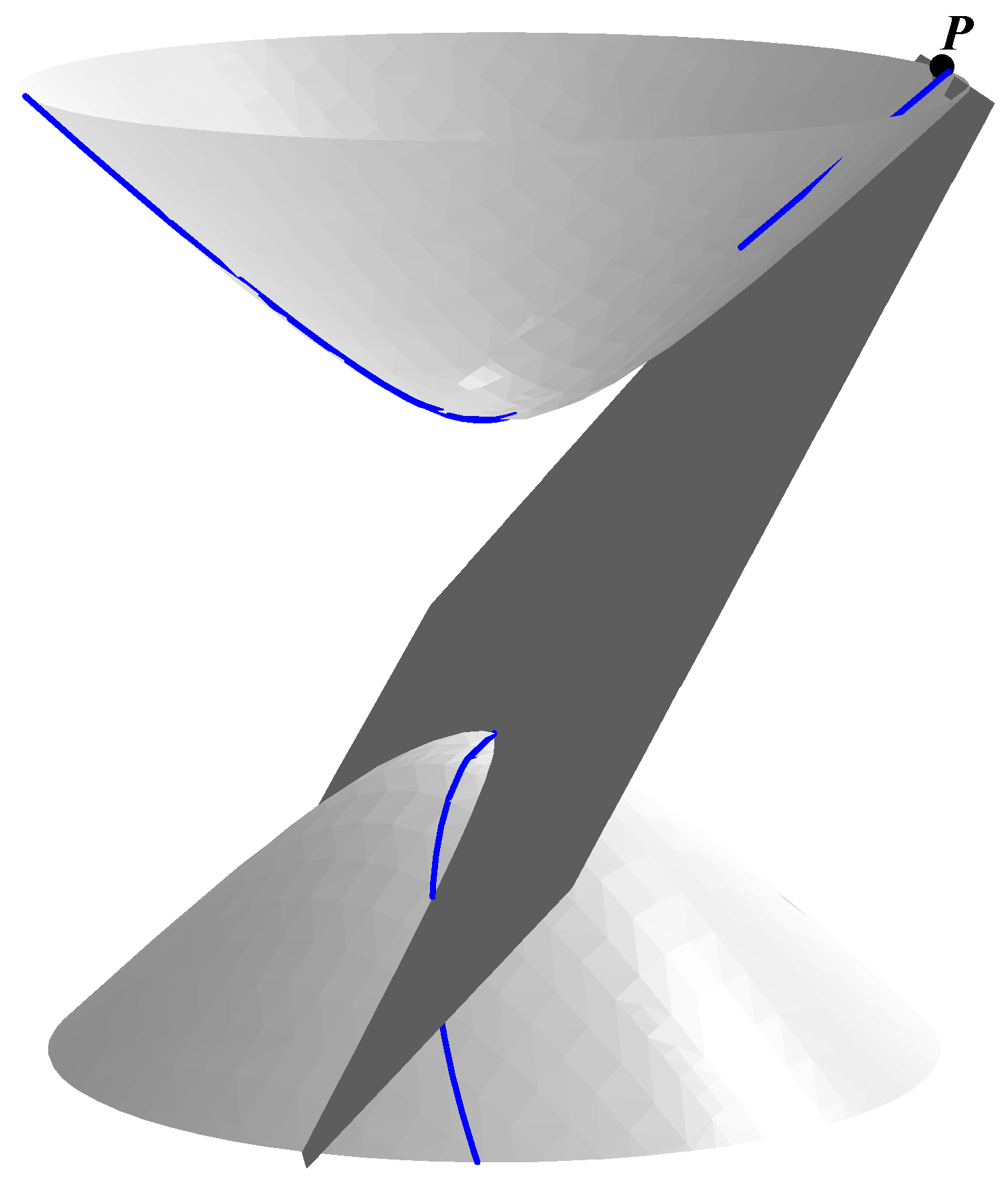
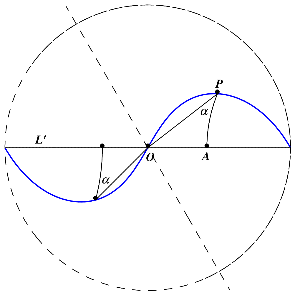
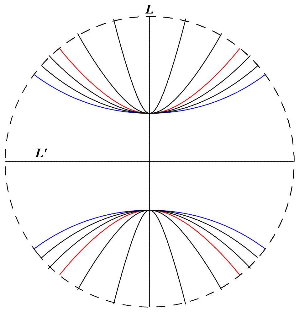
Since $Q_{\alpha }\left(\varphi \right)$ is real, it follows from Equation (2) that $R^Z=P{\oplus }_{\alpha }P$ is on ${\mathcal{H}}^{+}$ provided ${\cos }^2\varphi <\sin \alpha$. On the other hand, Figure 1 shows an example where R (and therefore $R^Z$) is on ${\mathcal{H}}^{-}$. Here, a typical $F_{\alpha }$ is shown (in blue) along with the S-line tangent at a point P.

Generally, if $P_1$ and $P_2$ are distinct points on ${\mathcal{H}}^{+}$ we will see (Section 5) that $R^Z$ is on ${\mathcal{H}}^{+}$, provided $\cos {\varphi }_1\cos {\varphi }_2<\sin \alpha$; it is sufficient, but not necessary, that $P_1$ and $P_2$ be in the open region $\mathcal{E}$ where $-1<X<1$ for this condition to hold. This condition is the setting for the Main Theorem because, as noted above, the ellipses are in $\mathcal{E}$. In Section 4, we map ${\mathcal{H}}^{+}$ to $\mathbb{D}$ by stereographic projection and show the image of $\mathcal{E}$ bounded by $E_1$ where $E_1$ is the image of $X=\pm 1$. 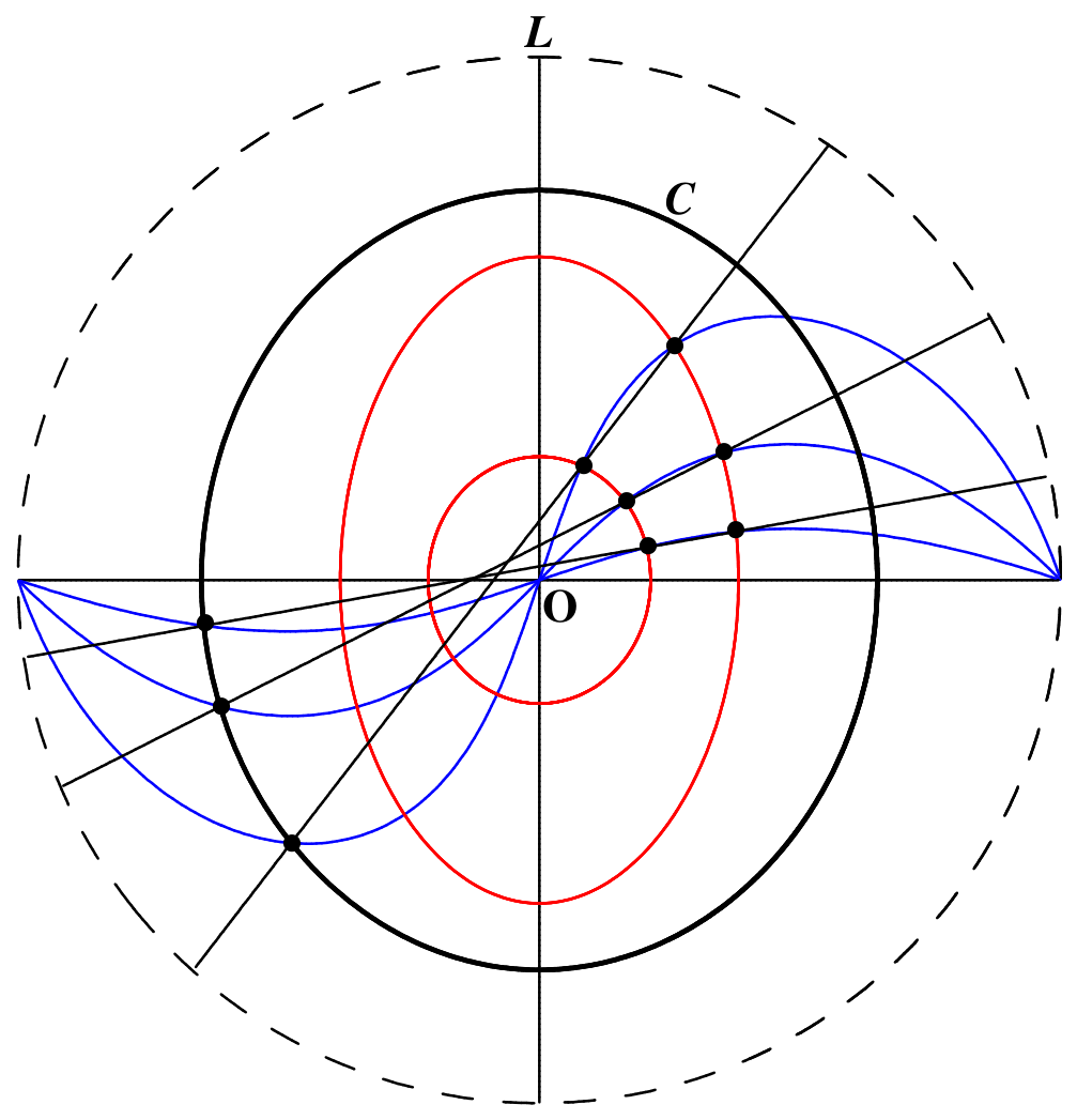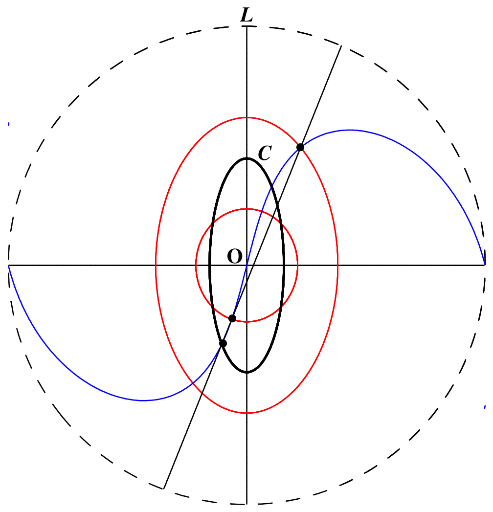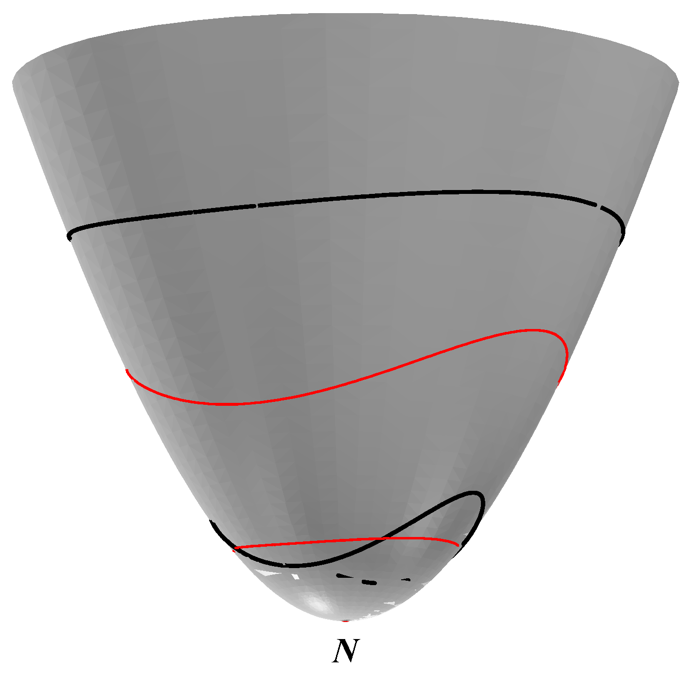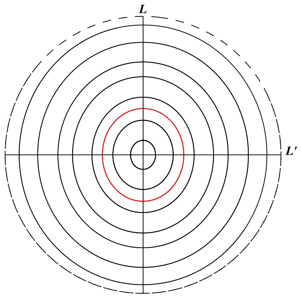Figure 2 is an illustration on ${\mathcal{H}}^{+}$ of the Main Theorem. The ellipses $E_{{\displaystyle \frac{1}{3}}}$ and $E_{{\displaystyle \frac{2}{3}}}$ are shown in red, with $E_{{\displaystyle \frac{1}{3}}}$ closer to $N=E_0$. Their compositions C for $\iota =\pm 1$ are shown in black. When $\iota =1$ the conic C does not intersect the component ellipses. When $\iota =-1$ the conic C intersects $E_{{\displaystyle \frac{1}{3}}}$ in four points.

4. Projection to Plane Curves

In this section we project the $F_{\alpha }$ into $\mathbb{D}$ and compute their orthogonal trajectories, which turn out to be the $E_{ϵ}$ as they were represented in [1]. Stereographic projection of $\mathcal{H}$ from $S=\left(0,0,-1\right)$ into ${\mathbb{R}}^2$ is given by

$$\left(X,Y,Z\right)\mapsto \left({\displaystyle \frac{X}{1+Z}},{\displaystyle \frac{Y}{1+Z}}\right)=\left(x,y\right)$$

which conformally maps ${\mathcal{H}}^{+}$ to the interior of $\mathbb{D}$ and ${\mathcal{H}}^{-}$ to the region outside the disk. Thus, N is mapped to $O=\left(0,0\right)$, and $L^{\prime }$ becomes the line $y=0$ in $\mathbb{D}$. From Equation (1), we find that the image of $F_{\alpha }$ is the polar curve

$$r^2={\displaystyle \frac{\cos \left(\alpha +\varphi \right)}{\cos \left(\alpha -\varphi \right)}}.$$

(3)

This is the non-singular cubic $F_{\alpha }\left(x,y\right)=0$, where

$$F_{\alpha }\left(x,y\right)=\left(x^2+y^2\right)\left(x+y\tan \alpha \right)-\left(x-y\tan \alpha \right)$$

(3a)

which has the single real asymptote $x\cot \alpha +y=0$. Figure 3 shows the portion in $\mathbb{D}$ of an $F_{\alpha }$ in blue. Angle $\alpha$ is shown at two typical points. The dashed line is the asymptote.

This representation of $F_{\alpha }$ as a cubic curve symmetric about O was chosen to make computation as simple as possible. However, our results are not representation dependent because the image of $F_{\alpha }$ by a Möbius transformation is either a cubic or an irreducible quartic with two ordinary singularities at non-real points. In particular, incidence is preserved and the elliptic curve addition law we derive would hold in either case.

We now show that the $F_{\alpha }$ and $E_{ϵ}$ are orthogonal trajectories of each other. Since stereographic projection is conformal, it follows from Equation (3) that the orthogonal trajectories of the $F_{\alpha }$ are the solutions to the polar equation

$$\left(\sin 2\varphi \right)d\varphi ={\displaystyle \frac{1-r^4}{2r^3}}dr.$$

These are the algebraic curves

$$r^4-2r^2\left(\cos 2\varphi +{\displaystyle \frac{2}{{ϵ}^2}}\right)+1=0$$

(4)

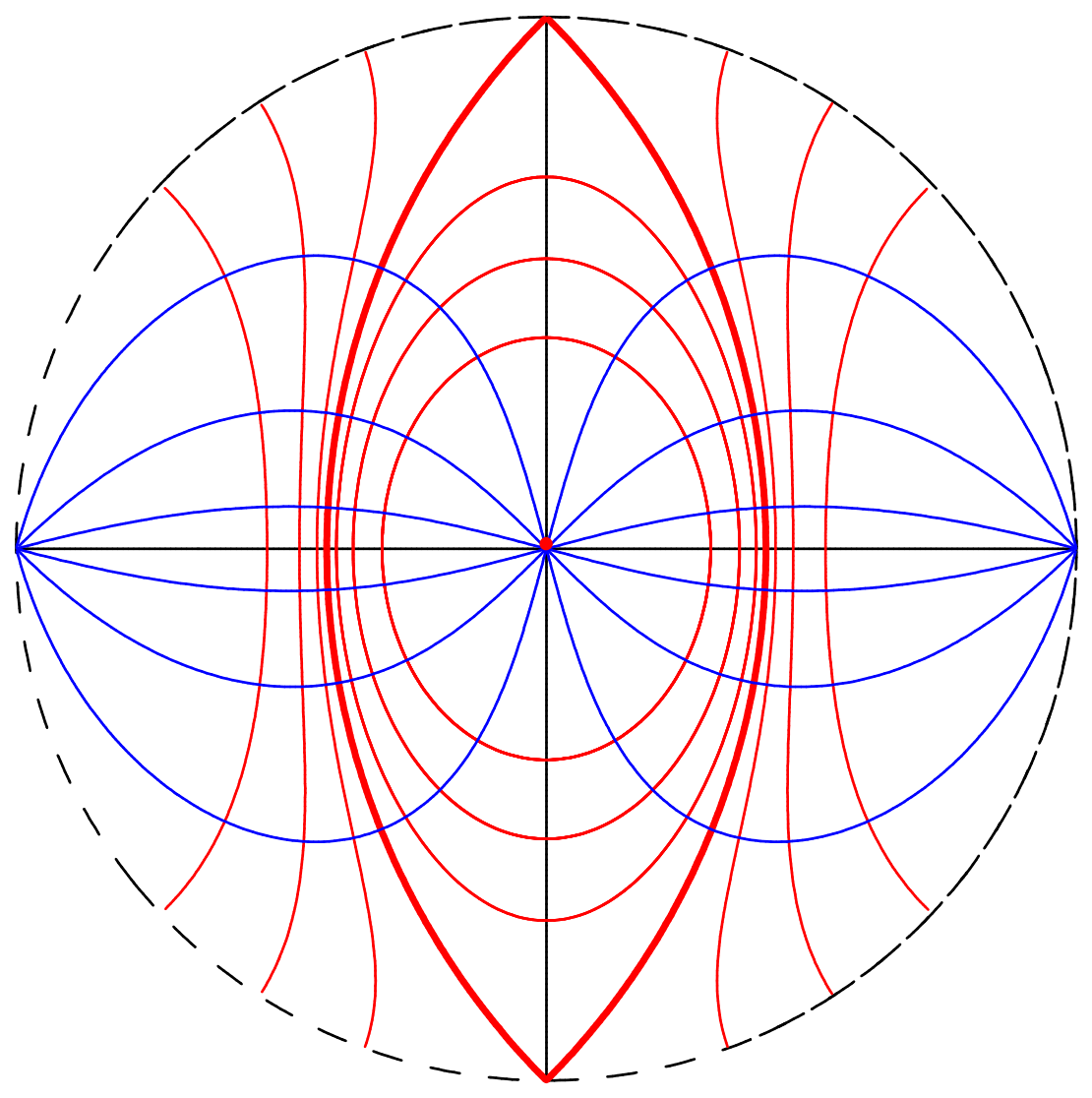
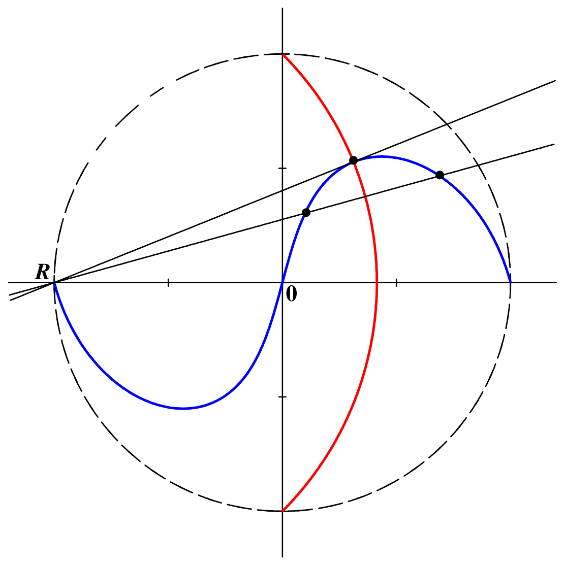
with parameter $ϵ$, which are the complete forms of the non-trivial $E_{ϵ}$ as derived in [1] (pp. 139–140). Figure 4 shows the portions in $\mathbb{D}$ of $F_{\alpha }$ (blue) and $E_{ϵ}$ (red). The curve $E_1$, shown in bold red, is the projection of the intersections with ${\mathcal{H}}^{+}$ of the planes $X=\pm 1$, the boundary of the open region $\mathcal{E}$ defined in Section 2. The ellipses are in $\mathcal{E}$.

We now identify $P=\left(x,y\right)$ with the complex number $x+iy$. The image of the transverse axis $L^{\prime }$ is the real line in $\mathbb{D}$ and the image of the focal axis L is the imaginary line. Writing $P^{*}$ for $x-iy$, the distance between two points $P_1$ and $P_2$ in $\mathbb{D}$ is given by

$$d\left(P_1,P_2\right)=\mathrm{arctanh}\left|{\displaystyle \frac{P_1-P_2}{1-P_1^{*}{P}_2}}\right|$$

(5)

which is equivalent to the Minkowski distance formula on ${\mathcal{H}}^{+}$ given by

$${\displaystyle \frac{1}{2}}\mathrm{arccosh}\left(Z_1{Z}_2-Y_1{Y}_2-X_1{X}_2\right).$$

Also, the complete curves $F_{\alpha }$ and $E_{ϵ}$ are invariant under the transformation $P\mapsto {\displaystyle \frac{1}{P}}$. For $F_{\alpha }$, this is equivalent of replacing $\varphi$ with $-\varphi$ in Equation (1), whereby ${\displaystyle \frac{1}{0}}$ is the ideal point for the real asymptote, with projective coordinates $\left[\tan \alpha :-1:0\right]$.

Remark 1.

The Möbius involution $P\mapsto {\displaystyle \frac{P-i}{iP-1}}$ maps $\mathbb{D}$ to the upper half-plane, its boundary to the real line, and the remaining points to the lower half-plane. The $F_{\alpha }$ are mapped to the one-loop Cassini ovals and the $E_{ϵ}$ to the two-loop ovals. From the algebraic classification of Cassini ovals it follows that the $F_{\alpha }$ and $E_{ϵ}$ represent all genus 1 curves with real coefficients, which are algebraically equivalent precisely when they have the same shape invariant, Klein’s j-invariant. The invariant j can be computed from the cross-ratio χ of an algebraically equivalent non-singular cubic; the curve is harmonic if $j=1$, suitably normalized. A single hyperbolic translation will transform every $F_a$ to Weierstrass normal form, from which standard formulas produce χ or any of its anharmonic forms, equivalent in that they correspond to the same j. One of these is $\chi =e^{4i\alpha }$, which implies $j\le 1$. The hyperbolic translation that takes $E_{ϵ}$ to a Weierstrass cubic depends on ϵ and leads to $\chi ={ϵ}^4$, which implies $j\ge 1$. Thus, there is no overlap by algebraic equivalence between the $F_{\alpha }$ and $E_{ϵ}$ except for the harmonic cases ($\alpha =\pm {\displaystyle \frac{\pi }{4}}$, $ϵ=2^{\pm {\displaystyle \frac{1}{4}}}$).

5. Composition of Ellipses

In this section we derive an explicit formula for the elliptic curve addition on $F_{\alpha }$ with points represented as complex numbers. First, we recall the simple form of Equation (2) in Section 3 and use it to prove a special case of the Main Theorem that motivates the composition of two ellipses in general. Specifically, with ${\cos }^2\varphi <\sin \alpha$, it is easy to find the composition of $E_{ϵ}$ with itself. We assume $\iota =1$ since the symmetry of $F_{\alpha }$ implies $E_{ϵ}{\circ }_{-1}{E}_{ϵ}=E_0=O$.

Proposition 1.

The composition $E_{ϵ}{\circ }_1{E}_{ϵ}$ is the circle with center O and radius $\mathrm{arctanh}ϵ$.

Proof. 

Let P be an intersection point of $F_{\alpha }$ with $E_{ϵ}$. Solving Equations (3) and (4) simultaneously, with ${\sin }^2\alpha \le {\cos }^2\varphi <\sin \alpha$ because $E_{ϵ}\subset \mathcal{E}$, yields

$${ϵ}^2{\sin }^{2}2\varphi =2\left(\cos 2\alpha +\cos 2\varphi \right).$$

(6)

From Equation (6) we find

$${\displaystyle \frac{1+{ϵ}^2}{1-{ϵ}^2}}={\displaystyle \frac{{\cos }^2\alpha -{\sin }^4\varphi }{{\sin }^2\alpha -{\cos }^4\varphi }}.$$

From Equation (2), the Z-coordinate of $P{\oplus }_{\alpha }P$ on ${\mathcal{H}}^{+}$ is

$$Z={\displaystyle \frac{1+{ϵ}^2}{1-{ϵ}^2}}.$$

Since $X^2+Y^2=Z^2-1$, it follows that

$$x^2+y^2={\left({\displaystyle \frac{X}{1+Z}}\right)}^2+{\left({\displaystyle \frac{Y}{1+Z}}\right)}^2={ϵ}^2,$$

the circle in $\mathbb{D}$ with center O and radius $\mathrm{arctanh}ϵ$. □

If $ϵ\ne 0$ then the vertices of $E_{ϵ}$ on its focal axis in $\mathbb{D}$ are $\pm {\displaystyle \frac{1}{ϵ}}\left(\sqrt{1-{ϵ}^2}-1\right)i$. It follows from the formula in Equation (5) that the radius of the circle in Proposition 1 is the length of the segment between these vertices. Consequently, any circle in ${\mathbb{H}}^2$ is the composition of a unique ellipse with itself, but no non-trivial circle is an ellipse. We now proceed under the assumptions that ${ϵ}_2\ne {ϵ}_1$ and ${ϵ}_1{ϵ}_2\ne 0$.

We now obtain a formula for $R^Z=P_1{\oplus }_{\alpha }{P}_2$ when $P_1\ne P_2$. This formula applies to the complete $F_{\alpha }$, with each point $P=x+iy$. First, the projection into $\mathbb{D}$ of the S-line through $P_1$ and $P_2$ is a chord of the unit circle whose points P satisfy

$$\left(P_1-P_2\right)P^{*}-\left(P_1^{*}-P_2^{*}\right)P=P_1{P}_2^{*}-P_2{P}_1^{*}.$$

(7)

Since N projects to the identity 0 we assume $P_1{P}_2\ne 0$. Next, from Equation (3a), $F_{\alpha }$ consists of all P such that

$$\left(P{P}^{*}-1\right)\left(P+P^{*}\right)=i\left(P{P}^{*}+1\right)\left(P-P^{*}\right)\tan \alpha .$$

(8)

Solving for $P^{*}$ in Equation (7) and substituting into Equation (8) produces a cubic polynomial in P with constant term $a_0$. Since $P_1$ and $P_2$ are on $F_{\alpha }$, the roots of this polynomial are obtained from the monic factorization $\left(P-P_1\right)\left(P-P_2\right)\left(P-R\right)$. Then $P_1{P}_{2}R=-a_0$ and $P_1{\oplus }_{\alpha }{P}_2=-R$. It follows after solving for R that

$$P_1{\oplus }_{\alpha }{P}_2={\displaystyle \frac{P_1-P_2}{P_1^{*}-P_2^{*}}}\left({\displaystyle \frac{P_1^{*}}{P_1}}-{\displaystyle \frac{P_2^{*}}{P_2}}\right){\displaystyle \frac{1}{\left(P_1-P_2\right)+e^{2i\alpha }\left(P_1^{*}-P_2^{*}\right)}}.$$

(9)

The formula in Equation (9) is undefined when ${\displaystyle \frac{P_2-P_1}{P_1^{*}-P_2^{*}}}=e^{2i\alpha }$. In this case, recall from Section 4 that $F_{\alpha }$ is invariant when the complex number representing a point is replaced by its reciprocal. Geometrically, this means that the S-line in Equation (7) through a point and its reciprocal is parallel in ${\mathbb{R}}^2$ to the asymptote $x\cot \alpha +y=0$; that is, if $P_1$ and $P_2$ are reciprocals as complex numbers then $P_1{\oplus }_{\alpha }{P}_2$ is the ideal point $\left[\tan \alpha :-1:0\right]$. Otherwise, from Equation (3), let $P_j=r_j{e}^{i{\varphi }_j}$. Then ${\left|{\displaystyle \frac{P_1^{*}}{P_1}}-{\displaystyle \frac{P_2^{*}}{P_2}}\right|}^2=2\left(1-\cos \left(2{\varphi }_1-2{\varphi }_2\right)\right)$. Thus ${\left|P_1{\oplus }_{\alpha }{P}_2\right|}^2$, which will be used in the proof of the Main Theorem, is determined by the denominator of the third factor in Equation (9). Noting that $\cos 2\alpha +\cos 2{\varphi }_j\ge 0$, there are two cases to consider depending on whether $\cos \left(\alpha -{\varphi }_1\right)$ and $\cos \left(\alpha -{\varphi }_2\right)$ have the same or opposite signs. For brevity we omit the straightforward calculation that yields

$${\left|\left(P_1-P_2\right)+e^{2i\alpha }\left(P_1^{*}-P_2^{*}\right)\right|}^2=2{\left(\sqrt{\cos 2\alpha +\cos 2{\varphi }_1}-\iota \sqrt{\cos 2\alpha +\cos 2{\varphi }_2}\right)}^2,$$

where $\iota =1$ in the same-sign case, and $\iota =-1$ otherwise. Therefore, with $Q_{\alpha }\left(\varphi \right)$ as in Section 3,

$${\left|P_1{\oplus }_{\alpha }{P}_2\right|}^2={\displaystyle \frac{1}{\cos 2\alpha +1}}{\displaystyle \frac{1-\cos \left(2{\varphi }_1-2{\varphi }_2\right)}{{\left(Q_{\alpha }\left({\varphi }_1\right)-\iota Q_{\alpha }\left({\varphi }_2\right)\right)}^2}}.$$

(10)

Proposition 2.

If $P_1$ and $P_2$ are on $F_{\alpha }$ in $\mathbb{D}$ then $P_1{\oplus }_{\alpha }{P}_2$ is in $\mathbb{D}$ if and only if $\cos {\varphi }_1\cos {\varphi }_2<\sin \alpha$.

Proof. 

Since $F_{\alpha }$ is symmetric about 0 it suffices to assume $P_1$ and $P_2$ are in the first polar quadrant of $\mathbb{D}$. The claim is obvious if $P_1$ and $P_2$ are in opposite quadrants because $\cos {\varphi }_1\cos {\varphi }_2<0$ in that case and $P_1{\oplus }_{\alpha }{P}_2$ is clearly in $\mathbb{D}$. Then $\iota =1$ in Equation (10). Instead of a tedious manipulation with identities, we show that the condition for $\left|P_1{\oplus }_{\alpha }{P}_2\right|<1$ is determined by the location of $P_1$ and $P_2$ relative to the portion of $E_1$ in this quadrant. First, if $P_1$ and $P_2$ are related by inversion in $E_1$, then

$$P_2={\displaystyle \frac{1-P_1^{*}}{1+P_1^{*}}}$$

whereby

$$\tan {\varphi }_2={\displaystyle \frac{2r_1}{1-r_1^2}}\sin {\varphi }_1.$$

Then, $\tan \alpha \tan {\varphi }_2=Q_{\alpha }\left({\varphi }_1\right)$, equivalently, $\cos {\varphi }_1\cos {\varphi }_2=\sin \alpha$. In this case, the S-line through $P_1$ and $P_2$ meets the boundary at $R=-1$, as shown in Figure 5 for $P_1=P_2$ on $E_1$ and for $P_1\ne P_2$. Now, if $P_2$ is replaced by any point $P\left(\varphi \right)$ on $F_{\alpha }$ in the first quadrant then the corresponding R is in $\mathbb{D}$ if and only if ${\varphi }_2>\varphi$, that is, $\cos \varphi \cos {\varphi }_2<\sin \alpha$. □

In particular, if $P_1$ and $P_2$ are both in $\mathcal{E}$ then $P_1{\oplus }_{\alpha }{P}_2$ is in $\mathbb{D}$, consistent with Proposition 1 and the statement of the Main Theorem.

6. The Computation Field

Typical of analytic geometry in the hyperbolic plane, the proof of the Main Theorem requires several algebraic identities that are straightforward but intricate. We establish these in this section. Although the dilation that transforms lines to S-lines also transforms ellipses to quadratic curves in $\mathbb{D}$, it also transforms each $F_{\alpha }$ to a quartic curve and offers no advantage in the proof. To keep the algebra manageable, we will adopt the following step-by-step procedure.

(1)

We view ${ϵ}_1$, ${ϵ}_2$, and $\cos 2\alpha$ as formal variables and work within an extension of the base field $\mathbb{Q}\left({ϵ}_1,{ϵ}_2,\cos 2\alpha \right)$. For $j=1$ or 2, let

$$\begin{array}{cc}\hfill {\beta }_j& ={ϵ}_j^2\cos 2\alpha -1\hfill \\ \hfill {\gamma }_j& ={ϵ}_j^4-2{\beta }_j-1.\hfill \end{array}$$

Adjoining $\sqrt{{\gamma }_1}$ and $\sqrt{{\gamma }_2}$ to the base field produces an extension K with basis $B_0=1$, $B_1=\sqrt{{\gamma }_1}$, $B_2=\sqrt{{\gamma }_2}$, $B_3=B_1{B}_2$.

(2)

Let $B_4=\sqrt{B_1+{\beta }_1}\sqrt{B_2+{\beta }_2}$. We will avoid explicit reference to the parameter $\alpha$ by performing computations in the field $K\left(B_4\right)$ where coefficients of the basis elements reduce to polynomials in ${\beta }_1$ and ${\beta }_2$ over the base field. It follows that each $B_j\ge 0$ if $\alpha$ and ${ϵ}_j$ are real numbers with $0\le {ϵ}_j<1$. The field elements and their definitions are displayed in Table 1.

(3)

We define an element $\rho$ in $K\left(B_4\right)$ that satisfies a quadratic polynomial over K, and conclude Section 6 with the statement of a pivotal lemma and its corollary. Their proofs require straightforward but lengthy field computations and are provided in the Appendix A.

(4)

In Section 7 we show that $\rho$ can be identified with ${\left|P_1{\oplus }_{\alpha }{P}_2\right|}^2$ in Equation (10). This is achieved by creating a quartic polynomial with symmetric coefficients (so its roots occur in reciprocal pairs). This quartic factors into two quadratics over K, one of which is the polynomial in step 3 above. Thus, the squared modulus of $P_1{\oplus }_{\alpha }{P}_2$ (and its reciprocal, as discussed in Section 2) are roots of this quadratic. This sets up the proof of the Main Theorem. The proof does not require the other quadratic factor whose roots can be shown to be on the unit circle. The relation of these ‘extraneous’ roots to the polar angle of $P_1{\oplus }_{\alpha }{P}_2$ is of potential interest but will not be discussed here.

Certain elements in $\mathbb{Q}\left({ϵ}_1,{ϵ}_2\right)$ will occur frequently as we manipulate the field relations. These include

$$\begin{array}{cc}\hfill \delta & ={ϵ}_1^2-{ϵ}_2^2\hfill \\ \hfill \sigma & ={ϵ}_1^2+{ϵ}_2^2\hfill \\ \hfill \tau & =\iota {ϵ}_1{ϵ}_2\hfill \\ \hfill \omega & =\tau +{\displaystyle \frac{1}{2}}\sigma \hfill \\ \hfill \lambda & ={\tau }^2+1\hfill \\ \hfill \mu & ={\tau }^2-1.\hfill \end{array}$$

For example, the elements ${\beta }_0:=2\tau \cos 2\alpha +\lambda$ and ${\gamma }_0:=2{\tau }^2\cos 2\alpha -\sigma$ can be written as they appear in Table 1:

$$\begin{array}{cc}\hfill {\beta }_0& =\lambda +{\displaystyle \frac{2\tau }{\delta }}\left({\beta }_1-{\beta }_2\right)\hfill \\ \hfill {\gamma }_0& ={ϵ}_2^2{\beta }_1+{ϵ}_1^2{\beta }_2.\hfill \end{array}$$

Also, the non-zero element $\delta$ can be expressed as ${\beta }_1{ϵ}_2^2-{\beta }_2{ϵ}_1^2$, so it follows directly from the definitions of the ${\beta }_j$ that the element

$$\Omega ={ϵ}_1^2\left({\beta }_2+1\right)-{ϵ}_2^2\left({\beta }_1+1\right)$$

is identically zero. We can now state the pivotal lemma and its corollary, whose proofs are provided in Appendix A. The proofs use computations $\mathrm{mod}\left(\mathrm{\Omega }\right)$, where $\left(\mathrm{\Omega }\right)$ consists of all multiples of $\mathrm{\Omega }$. For example,

$${\gamma }_0=\tau \left({\beta }_0-\mu \right)-2\omega$$

(11)

because subtracting the RHS from the LHS produces ${\displaystyle \frac{\sigma }{\delta }}\mathrm{\Omega }$. Similarly,

$$\tau {\gamma }_1{\gamma }_2={\beta }_0\left({\gamma }_0+\tau \mu \right)+2\omega \left(\tau {\gamma }_0-\mu \right)$$

(12)

because subtraction produces ${\displaystyle \frac{1}{\delta }}\left(2\tau \left({\beta }_1+{\beta }_2\right)+4{\tau }^3+\sigma \mu -{\sigma }^2\tau \right)\mathrm{\Omega }$.

Lemma 1.

Let $U_1=\mu +B_1+B_2-B_3$ and $U_2={\gamma }_0+{ϵ}_2^2{B}_1+{ϵ}_1^2{B}_2$. Then

$$\left(\tau {\beta }_0-2\omega +\tau B_3\right)U_1=\left(2\tau \omega -{\beta }_0-B_3\right)U_2.$$

Corollary 1.

Let $\rho ={\displaystyle \frac{U_1-2B_4}{U_2-2\tau B_4}}$. Then ${\rho }^2-{\displaystyle \frac{{\beta }_0+B_3}{\omega }}\rho +1=0$.

7. Proof of the Main Theorem

In this section we assume $0\le {ϵ}_1\le {ϵ}_2$ and begin with an illustration in $\mathbb{D}$ of $C=C_{\iota }\left(\kappa ,\eta \right)$ for the two cases $\iota =\pm 1$. Figure 6 shows ellipses $E_{{ϵ}_1}$ and $E_{{ϵ}_2}$ (red) and S-lines through $P_1=E_{{ϵ}_1}\cap F_{\alpha }$ and $P_2=E_{{ϵ}_2}\cap F_{\alpha }$, for various $F_{\alpha }$ (blue) when $P_1$ and $P_2$ are in the same half-plane of the focal axis L. The third intersection with each $F_{\alpha }$ is shown on C (black) in the opposite half-plane, so $P_1{\oplus }_{\alpha }{P}_2$, the reflection in O of the third intersection, is also on C.

If $\iota =-1$ then C intersects $E_{{ϵ}_1}$ at four points, as shown in Figure 7 for the same two ellipses (red) and a typical $F_{\alpha }$ (blue) when $P_1$ and $P_2$ are in opposite half-planes of L.

Remark 2.

By symmetry, C is produced without reflecting the third intersection with each $F_{\alpha }$ in O. We have followed the definition of elliptic curve addition to ensure associativity in Section 9, where the ellipses will be viewed as oriented figures with a group structure.

Proof of the MainTheorem.

Let $\pm i\tanh {\displaystyle \frac{\eta }{2}}$ be the foci of $C_{\iota }\left(\kappa ,\eta \right)$ in the theorem, and let $\epsilon ={\displaystyle \frac{\tanh \eta }{\tanh \kappa }}$. A direct calculation using Equation (5) shows that $C_{\iota }\left(\kappa ,\eta \right)$ is described by the polar equation

$${\displaystyle \frac{1+r^4}{2r^2}}={\displaystyle \frac{2-{\epsilon }^2-{\tanh }^2\kappa +\left({\epsilon }^2-{\tanh }^2\eta \right)\cos 2\theta }{{\tanh }^2\kappa -{\tanh }^2\eta }}.$$

(13)

The proof proceeds in four steps.

Step 1. Noting that neither $\lambda +2\tau$ nor $\mu$ can be 0 (using the notation displayed in Section 6), the theorem asserts that

$$\begin{array}{cc}\hfill {\tanh }^2\kappa & ={\displaystyle \frac{\sigma +2\tau }{\lambda +2\tau }}\hfill \\ \hfill {\tanh }^2\eta & ={\displaystyle \frac{{\delta }^2}{{\mu }^2}}.\hfill \end{array}$$

Also, $\sigma -2\tau$ cannot be 0 so, from Equation (13), we have

$$\cos 2\theta ={\displaystyle \frac{\omega r^4-2\lambda r^2+\omega }{\left(\sigma -2\tau \right)r^2}}.$$

(14)

Step 2. Let $\phi$ be the polar angle for $P_1{\oplus }_{\alpha }{P}_2$ and let $\rho ={\left|P_1{\oplus }_{\alpha }{P}_2\right|}^2$. Since $P_1$ and $P_2$ are on $F_{\alpha }$ it follows from Equation (3), with $\rho ={\displaystyle \frac{\cos \left(\alpha +\phi \right)}{\cos \left(\alpha -\phi \right)}}$, that

$$\cos 2\phi ={\displaystyle \frac{\left(1+{\rho }^2\right)\cos 2\alpha -2\rho }{2\rho \cos 2\alpha -\left(1+{\rho }^2\right)}}.$$

(15)

(Note that $1+{\rho }^2$ cannot equal $2\rho \cos 2\alpha$.) We will show that $\cos 2\phi$ in Equation (15) is equal to $\cos 2\theta$ in Equation (14) when $r^2=\rho$.

Step 3. The alleged equality in Step 2 is equivalent to

$${\rho }^4-{\displaystyle \frac{2}{\omega }}\left(\lambda +2\tau \cos 2\alpha \right){\rho }^3+2{\displaystyle \frac{4\tau -\omega +2\lambda \cos 2\alpha }{\omega }}{\rho }^2-{\displaystyle \frac{2}{\omega }}\left(\lambda +2\tau \cos 2\alpha \right)\rho +1=0$$

because $\sigma =2\left(\omega -\tau \right)$ and $\omega$ cannot be 0. The coefficients are in the base field but the quartic polynomial in $\rho$ will factor into two quadratics after we express the coefficients in terms of basis elements for K. First, recall that $\lambda +2\tau \cos 2\alpha ={\beta }_0$, so the coefficient of the odd powers of $\rho$ is $-2{\displaystyle \frac{{\beta }_0}{\omega }}$. We claim that

$$4\omega \left(2\tau -\omega +\lambda \cos 2\alpha \right)={\beta }_0^2-B_3^2$$

which would rewrite the coefficient of ${\rho }^2$ as $2+{\displaystyle \frac{{\beta }_0^2-B_3^2}{{\omega }^2}}$. To see this, note that the LHS reduces to $4\lambda \omega \cos 2\alpha -{\delta }^2$, whereas the RHS is equal to

$${\left(\lambda +2\tau \cos 2\alpha \right)}^2-{\gamma }_1{\gamma }_2.$$

However, ${\gamma }_1{\gamma }_2=4{\tau }^2{\cos }^{2}2\alpha -2\lambda \sigma \cos 2\alpha +\left({ϵ}_1^4+1\right)\left({ϵ}_2^4+1\right)$ because ${\gamma }_j={ϵ}_j^4-2{ϵ}_j^2\cos 2\alpha +1$, so the RHS reduces to

$$2\lambda \left(2\tau +\sigma \right)\cos 2\alpha -{\left({ϵ}_1^2-{ϵ}_2^2\right)}^2=4\lambda \omega \cos 2\alpha -{\delta }^2.$$

The quartic is now

$${\rho }^4-2{\displaystyle \frac{{\beta }_0}{\omega }}{\rho }^3+\left(2+{\displaystyle \frac{{\beta }_0^2-B_3^2}{{\omega }^2}}\right){\rho }^2-2{\displaystyle \frac{{\beta }_0}{\omega }}\rho +1$$

which factors over K as

$$\left({\rho }^2-\rho {\displaystyle \frac{{\beta }_0+B_3}{\omega }}+1\right)\left({\rho }^2-\rho {\displaystyle \frac{{\beta }_0-B_3}{\omega }}+1\right).$$

By Corollary 1, the theorem is proved if we show that $\rho ={\displaystyle \frac{U_1-2B_4}{U_2-2\tau B_4}}$.

Step 4. As in Lemma 1, let $U_1=\mu +B_1+B_2-B_3$ and $U_2={\gamma }_0+{ϵ}_2^2{B}_1+{ϵ}_1^2{B}_2$. We will express $\rho$ as an element of $K\left(B_4\right)$. First, we solve for $\cos 2\varphi$ in Equation (6). Of the two solutions only

$$\cos 2\varphi ={\displaystyle \frac{1}{{ϵ}^2}}\left(\sqrt{{ϵ}^4-2{ϵ}^2\cos 2\alpha +1}-1\right)$$

is possible. Since ${\gamma }_j={ϵ}_j^4-2{ϵ}_j^2\cos 2\alpha +1$ it follows from $B_j=\sqrt{{\gamma }_j}$ that

$$\begin{array}{cc}\hfill \cos 2{\varphi }_1& ={\displaystyle \frac{B_1-1}{{ϵ}_1^2}}\hfill \\ \hfill \cos 2{\varphi }_2& ={\displaystyle \frac{B_2-1}{{ϵ}_2^2}}.\hfill \end{array}$$

Next, from Equation (10) and $\tau =\iota {ϵ}_1{ϵ}_2$ we have

$$\begin{array}{cc}\hfill \rho & ={\displaystyle \frac{1}{\cos 2\alpha +1}}{\displaystyle \frac{1-\cos \left(2{\varphi }_1-2{\varphi }_2\right)}{{\left(Q_{\alpha }\left({\varphi }_1\right)-\iota Q_{\alpha }\left({\varphi }_2\right)\right)}^2}}\hfill \\ \hfill & ={\displaystyle \frac{1-\cos \left(2{\varphi }_1-2{\varphi }_2\right)}{2\cos 2\alpha +\cos 2{\varphi }_1+\cos 2{\varphi }_2-\frac{2\tau }{{ϵ}_1{ϵ}_2}\sqrt{\cos 2\alpha +\cos 2{\varphi }_1}\sqrt{\cos 2\alpha +\cos 2{\varphi }_2}}}.\hfill \end{array}$$

To write $\rho$ in basis form we use

$$\cos 2\alpha +\cos 2{\varphi }_j={\displaystyle \frac{B_j+{\beta }_j}{{ϵ}_j^2}}.$$

Then, since ${\gamma }_0={ϵ}_2^2{\beta }_1+{ϵ}_1^2{\beta }_2$ and $B_4=\sqrt{B_1+{\beta }_1}\sqrt{B_2+{\beta }_2}$,

$$\rho ={\displaystyle \frac{{\tau }^2\left(1-\cos \left(2{\varphi }_1-2{\varphi }_2\right)\right)}{{\gamma }_0+{ϵ}_2^2{B}_1+{ϵ}_1^2{B}_2-2\tau B_4}}$$

so the denominator is $U_2-2\tau B_4$.

To complete the proof we must show that the numerator is $U_1-2B_4$. However, ${\tau }^2\left(1-\cos 2{\varphi }_1\cos 2{\varphi }_2\right)=\mu +B_1+B_2-B_3=U_1$, so it remains to show that ${\tau }^2\sin 2{\varphi }_1\sin 2{\varphi }_2=2B_4$. Note that $\sin 2{\varphi }_1$ and $\sin 2{\varphi }_2$ have the same sign whether $P_1$ and $P_2$ are in the same or opposite quadrants of the disk. It suffices, then, to let $\sin 2{\varphi }_j=\sqrt{1-{\cos }^{2}2{\varphi }_j}$, whereby

$$\begin{array}{cc}\hfill {\tau }^2\sin 2{\varphi }_1\sin 2{\varphi }_2& =\sqrt{{ϵ}_1^4-1-{\gamma }_1+2B_1}\sqrt{{ϵ}_2^4-1-{\gamma }_2+2B_2}\hfill \\ \hfill & =2\sqrt{B_1+{\beta }_1}\sqrt{B_2+{\beta }_2}=2B_4.\hfill \end{array}$$

Thus, $\rho ={\displaystyle \frac{U_1-2B_4}{U_2-2\tau B_4}}$ and the theorem is proved. □

Corollary 2 (Corollary to the proof).

Let $ϵ={\displaystyle \frac{\iota {ϵ}_1+{ϵ}_2}{1+\iota {ϵ}_1{ϵ}_2}}$. Then $E_{ϵ}$ is tangent to $E_{{ϵ}_1}{\circ }_{\iota }{E}_{{ϵ}_2}$ at its vertices on L.

Proof. 

Let $\theta$ be the polar angle for $E_{ϵ}$ and for $E_{{ϵ}_1}{\circ }_{\iota }{E}_{{ϵ}_2}$. Since r cannot be 0 for these curves we can eliminate it from simultaneous Equation (4) with Equation (13). This results in a linear equation in $\cos 2\theta$. With ${\tanh }^2\eta ={\displaystyle \frac{{\delta }^2}{{\mu }^2}}$ and ${\tanh }^2\kappa ={\displaystyle \frac{\sigma +2\tau }{\lambda +2\tau }}={ϵ}^2$, as in the proof of the theorem, it follows directly that $\cos 2\theta =-1$. Thus, $E_{ϵ}$ intersects $E_{{ϵ}_1}{\circ }_{\iota }{E}_{{ϵ}_2}$ only at their vertices on L. □

Remark 3.

Note that $\rho =\rho \left(\iota \right)$ and $\rho \left(1\right)>\rho \left(-1\right)$, as shown in Figure 6 and Figure 7.

Corollary 3.

$C_{\iota }\left(\kappa ,\eta \right)$ is the composition of a unique pair of ellipses. An ellipse is the composition only of itself with $E_0$.

Proof. 

Let $C_{\iota }\left(\kappa ,\eta \right)=E_{{ϵ}_1}{\circ }_{\iota }{E}_{{ϵ}_2}$ and let $\epsilon ={\displaystyle \frac{\tanh \eta }{\tanh \kappa }}$. We show that $\left({\kappa }_1,{\kappa }_2\right)\mapsto \left(\kappa ,\epsilon \right)$ is injective for $0\le {\kappa }_1\le {\kappa }_2$. The theorem implies $\epsilon =\tanh \left({\kappa }_2-\iota {\kappa }_1\right)$. Further, if ${\tanh }^2\kappa >\tanh \eta$ then $\iota =1$, equivalently, $\kappa >\mathrm{arctanh}\epsilon$; if ${\tanh }^2\kappa <\tanh \eta$ then $\iota =-1$, equivalently, $\kappa <\mathrm{arctanh}\epsilon$. Thus $\kappa ={\kappa }_2+\iota {\kappa }_1$ has the unique solution

$$\begin{array}{cc}\hfill {\kappa }_1& ={\displaystyle \frac{\iota }{2}}\left(\kappa -\mathrm{arctanh}\epsilon \right)\hfill \\ \hfill {\kappa }_2& ={\displaystyle \frac{1}{2}}\left(\kappa +\mathrm{arctanh}\epsilon \right)\hfill \end{array}$$

which shows, in particular, that ${\kappa }_1=0$ and ${\kappa }_2=\kappa$ if ${\tanh }^2\kappa =\tanh \eta$, that is, if $C_{\iota }\left(\kappa ,\eta \right)$ is an ellipse.$\square$

8. Split Inversion and Central Conics

In this section, corollaries to the Main Theorem will produce representatives for the central conics in the remaining categories listed in Section 2. We denote the split inversion of a conic C in its focal axis by $C^{‡}$, and in its transverse axis by $C_{‡}$. We will see that the categories are related by these inversions, as summarized in

Table 2. Construction of central conics.

Construction	Category	KC-Description
$E_{{ϵ}_1}{\circ }_{\iota }{E}_{{ϵ}_2}$	C4	Ellipse
$E_{ϵ}{\circ }_{\iota }{E}_{ϵ}$	C10	Circle
${\left(E_{{ϵ}_1}{\circ }_{\iota }{E}_{{ϵ}_2}\right)}^{‡}$	C2	Concave hyperbola
${\left(E_{{ϵ}_1}{\circ }_{\iota }{E}_{{ϵ}_2}\right)}_{‡}$	C1	Convex hyperbola
$E_{ϵ}{\circ }_{\iota }{E}_1$	C9	Equidistant curves

. Since we reserved the terms ellipse, hyper-ellipse, and hyperbola for Steiner conics, we will add the prefix KC to the descriptions of categories C1, C2, and C4; for example, the conics in C4 are the KC-ellipses $C=C_{\iota }\left(\kappa ,\eta \right)$, each of which is the composition of a unique pair of ellipses (Corollary 3). For the C in C4, it was shown in [1] (pp. 140–142) that the $C^{‡}$ comprise C2 (KC-concave hyperbolas) and the $C_{‡}$ comprise C1 (KC-convex hyperbolas). It was also shown that each $C_{‡}$ is the locus of points ${\overline{C}}_{\iota }\left({\kappa }^{\prime },{\eta }^{\prime }\right)$ the difference of whose distances from two foci is ${\kappa }^{\prime }\ne 0$ with ${\eta }^{\prime }\ne 0$ the distance between the foci. This locus is related to $C_{\iota }\left(\kappa ,\eta \right)$ by

$$\begin{array}{cc}\hfill \cosh {\kappa }^{\prime }& =\coth \kappa \hfill \\ \hfill \cosh {\eta }^{\prime }& =\coth \eta .\hfill \end{array}$$

(16)

In particular, if $ϵ\ne 0$ then ${\left(E_{ϵ}\right)}_{‡}$ is a hyperbola, distinguished among the ${\overline{C}}_{\iota }\left({\kappa }^{\prime },{\eta }^{\prime }\right)$ by $\cosh {\eta }^{\prime }={\cosh }^2{\kappa }^{\prime }$, equivalently, ${\displaystyle \frac{\tanh {\eta }^{\prime }}{\tanh {\kappa }^{\prime }}}=\sqrt{1+{ϵ}^2}$.

Remark 4.

The KC-concave hyperbolas are also the split inversions of the KC-convex hyperbolas in their focal axes. Specifically, ${\left({\left(E_{{ϵ}_1}{\circ }_{\iota }{E}_{{ϵ}_2}\right)}_{‡}\right)}^{‡}$ is congruent to ${\left(E_{{ϵ}_1}{\circ }_{\iota }{E}_{{ϵ}_2}\right)}^{‡}$ by reflection in the asymptotes of the hyperbolas ${\left(E_{ϵ}\right)}_{‡}$.

Corollary 4.

The locus ${\left(E_{ϵ}{\circ }_1{E}_{ϵ}\right)}_{‡}$ is a pair of ultra-parallel lines.

Proof. 

Let ${\left(E_{ϵ}\right)}_{‡}$ represent the hyperbola, for some $0<ϵ<1$. Proposition 1 shows that $E_{ϵ}{\circ }_1{E}_{ϵ}$ is a circle of radius $\mathrm{arctanh}ϵ$, so category C10 consists of compositions of ellipses with each other. Furthermore, the split inversion of a circle across a diameter line yields a pair of lines perpendicular to that diameter, since the inversion is conformal. Thus, ${\left(E_{ϵ}{\circ }_1{E}_{ϵ}\right)}_{‡}$ is a pair of ultra-parallel lines with the focal axis of the hyperbola as the common perpendicular. □

Remark 5.

With $ϵ=\tanh \kappa$, the distance between the lines ${\left(E_{ϵ}{\circ }_1{E}_{ϵ}\right)}_{‡}$ is $\mathrm{arctanh}\left(sech2\kappa \right)$. This accounts for category C9B.

The remaining categories, C9 and C9A, are obtained from the Main Theorem by continuity, as compositions of ellipses with the boundary of $\mathcal{E}$. The proof of the following corollary is straightforward.

Corollary 5.

The composition $E_{ϵ}{\circ }_{\iota }{E}_1$ is the reducible curve represented in $\mathbb{D}$ by

$$x^2+y^2=1\pm 2x{\displaystyle \frac{1-\iota ϵ}{1+\iota ϵ}},$$

which is contained in $\mathcal{E}$ if $\iota =-1$, and outside of $\mathcal{E}$ if $\iota =1$. This is a pair of equidistant curves that meet the focal axis at angle $\arctan {\displaystyle \frac{1+\iota ϵ}{1-\iota ϵ}}$, from which it follows that ${\left(E_{ϵ}{\circ }_{\iota }{E}_1\right)}_{‡}$ is the pair of intersecting lines

$$y=\pm {\displaystyle \frac{1-\iota ϵ}{1+\iota ϵ}}x.$$

Categories C9A (intersecting lines) and C9B (ultra-parallel lines) are degenerate cases in the sense that they arise as KC-conics from degenerate cones, whereas C9 (equidistant curves) arise from cones tangent to the boundary of a hyperbolic domain. To summarize, the composition of an ellipse with the equidistant curves $E_1$ yields another pair of curves equidistant from the focal axis, and the split inversion of these curves across the transverse axis is in C9A. According to Proposition 1, if $ϵ\ne 0$ then the composition of $E_{ϵ}$ with itself for $\iota =1$ is a circle whose split inversion in the transverse axis is in C9B. The constructions that produce the non-degenerate central conics are summarized in Table 2, where $C^{‡}$ ($C_{‡}$) is the split inversion of C in its focal (transverse) axis.

9. The Group of Steiner Conics

The lines perpendicular to a given line L in ${\mathbb{H}}^2$ comprise an ultra-parallel pencil. Reflections in the lines of this pencil generate a subgroup $G\left(L\right)$ of collineations. The identity component of this group is denoted by $G_0\left(L\right)$. The identity component consists of translations, which are products of an even number of reflections. In this section we use the Main Theorem to identify $G\left(L\right)$ with ${\mathcal{D}}_0\cup \mathcal{O}$ (see Section 1) and $G_0\left(L\right)$ with ${\mathcal{D}}_0$. In light of Remark 4, we restrict our attention to the conics with locus descriptions $C_{\iota }\left(\kappa ,\eta \right)$ and ${\overline{C}}_{\iota }\left({\kappa }^{\prime },{\eta }^{\prime }\right)$.

To obtain this representation we identify each ellipse in ${\mathcal{D}}_0$ with a translation in $G_0\left(L\right)$, and each hyperbola in $\mathcal{O}$ with a single reflection. First, with $\kappa \in \mathbb{R}$ the group of translations along L consists of the Möbius transformations

$$g\left(\kappa ,Z\right)={\displaystyle \frac{Z+i\tanh \kappa }{1-Zi\tanh \kappa }}.$$

With $ϵ=\tanh \kappa$, we want $E_{ϵ}$ to represent $g\left(\kappa ,Z\right)$. Then $E_0$ would represent $g\left(0,Z\right)$ and the inverse of $E_{ϵ}$ must be defined to represent $g\left(-\kappa ,Z\right)$. We define it in accordance with $E_{ϵ}{\circ }_{-1}{E}_{ϵ}=E_0$ by giving an ellipse two orientations, $E_{ϵ}$ and $E_{-ϵ}$. With this convention, explicit reference to $\iota =\pm 1$ is no longer needed. Accordingly, $E_{{ϵ}_1}\circ E_{{ϵ}_2}$ will denote the composition C of $E_{{ϵ}_1}$ and $E_{{ϵ}_2}$, with ${ϵ}_1$ and ${ϵ}_2$ taking independent values in $\left(-1,1\right)$. Since $g\left({\kappa }_2,g\left({\kappa }_1,Z\right)\right)=g\left({\kappa }_1+{\kappa }_2,Z\right)$, we represent this translation by $E_{ϵ}$ with $ϵ={\displaystyle \frac{{ϵ}_1+{ϵ}_2}{1+{ϵ}_1{ϵ}_2}}$. By the corollary to the proof of the Main Theorem, $E_{ϵ}$ is the unique ellipse containing the vertices of $C=E_{{ϵ}_1}\circ E_{{ϵ}_2}$ on L. We denote it by $\pi \left(C\right)$. Considering $E_{ϵ}$ to be tangent to itself, we summarize this paragraph as follows.

Proposition 3.

Let $C=E_{{ϵ}_1}\circ E_{{ϵ}_2}$ and let $\pi \left(C\right)$ be the unique (oriented) ellipse tangent to C at its intersections with L. Then $\pi \left(C\right)$ represents $g\left({\kappa }_2,g\left({\kappa }_1,Z\right)\right)$ in the commutative group $G_0\left(L\right)$.

The elements of $G\left(L\right)$ not in the identity component are reflections. For $\kappa >0$, the involution

$$h\left(\kappa ,Z\right)={\displaystyle \frac{Z^{*}\cosh \kappa +i}{\cosh \kappa -Z^{*}i}}$$

is the reflection in the line perpendicular to L at $i{e}^{-\kappa }$. The reflection in the line perpendicular to L at $-i{e}^{-\kappa }$ is

$$\overline{h}\left(\kappa ,Z\right)={\displaystyle \frac{Z^{*}\cosh \kappa -i}{\cosh \kappa +Z^{*}i}}=-h\left(\kappa ,-Z\right).$$

Since $Z\mapsto Z^{*}$ is the reflection in $L^{\prime }$ we will denote it by $h\left(\infty \right)=\overline{h}\left(\infty \right)$ and refer to it as the absolute reflection. For brevity, we now express compositions in $G\left(L\right)$ in product form without Z in the notation. Thus, $g\left({\kappa }_2\right)g\left({\kappa }_1\right):=g\left({\kappa }_2,g\left({\kappa }_1,Z\right)\right)$. In particular, let ${\kappa }_j^{\prime }=\mathrm{arctanh}\mathrm{sech}\kappa$. Then $h\left(\kappa \right)h\left(\infty \right)=g\left({\kappa }^{\prime }\right)=h\left(\infty \right)\overline{h}\left(\kappa \right)$, and so $h\left(\infty \right)h\left(\kappa \right)=g\left(-{\kappa }^{\prime }\right)=\overline{h}\left(\kappa \right)h\left(\infty \right)$.

To extend Proposition 3 we identify each reflection with a hyperbola ${\left(E_{ϵ}\right)}_{‡}$. With $\kappa >0$ and $ϵ=\tanh \kappa$, let $h\left(\kappa \right)$ and $\overline{h}\left(\kappa \right)$ be represented respectively by the oppositely oriented hyperbolas ${\left(E_{ϵ}\right)}_{‡}$ and ${\left(E_{-ϵ}\right)}_{‡}$. Equivalently, from Equation (16), this determines a correspondence between $h\left(\kappa \right)$ and $g\left({\kappa }^{\prime }\right)$ with $\tanh {\kappa }^{\prime }=\mathrm{sech}\kappa$, and between $\overline{h}\left(\kappa \right)$ and $g\left({\kappa }^{\prime }\right)$ with $\tanh {\kappa }^{\prime }=-\mathrm{sech}\kappa$. Previously, we did not define ${\left(E_0\right)}_{‡}$ because it would consist of the absolute points $\pm i$, but here it represents $h\left(\infty \right)$ as the degenerate absolute hyperbola.

With these assignments we complete the representation of $G\left(L\right)$, beginning with the products of non-absolute reflections. These are straightforward. With $\tanh {\kappa }_j^{\prime }={ϵ}_j^{\prime }=\mathrm{sech}{\kappa }_j$ in all cases, they are listed in

Table 3. Products of Two Reflections.

Reflections	Product	Representative
$h\left({\kappa }_2\right)h\left({\kappa }_1\right)$	$g\left({\kappa }_2^{\prime }-{\kappa }_1^{\prime }\right)$	$\pi \left(E_{-{ϵ}_1^{\prime }}\circ E_{{ϵ}_2^{\prime }}\right)$
$\overline{h}\left({\kappa }_2\right)\overline{h}\left({\kappa }_1\right)$	$g\left({\kappa }_1^{\prime }-{\kappa }_2^{\prime }\right)$	$\pi \left(E_{{ϵ}_1^{\prime }}\circ E_{-{ϵ}_2^{\prime }}\right)$
$h\left({\kappa }_2\right)\overline{h}\left({\kappa }_1\right)$	$g\left({\kappa }_1^{\prime }+{\kappa }_2^{\prime }\right)$	$\pi \left(E_{{ϵ}_1^{\prime }}\circ E_{{ϵ}_2^{\prime }}\right)$
$\overline{h}\left({\kappa }_2\right)h\left({\kappa }_1\right)$	$g\left(-{\kappa }_2^{\prime }-{\kappa }_1^{\prime }\right)$	$\pi \left(E_{-{ϵ}_1^{\prime }}\circ E_{-{ϵ}_2^{\prime }}\right)$

along with the ellipses that represent them.

Representing the product of a translation and a non-absolute reflection is more intricate, as indicated by the following proposition. Since split inversion respects tangency we set $\pi \left(C_{‡}\right):=\pi {\left(C\right)}_{‡}$ for C in category C4. This is the unique (oriented) hyperbola tangent to $C_{‡}$ at its intersections with L.

Proposition 4.

If $\cosh {\kappa }_2\tanh {\kappa }_1<1$ then the reflection $h\left({\kappa }_2\right)g\left({\kappa }_1\right)$ is represented by $\pi {\left(E_{{ϵ}_1^{\prime }}\circ E_{{ϵ}_2^{\prime }}\right)}_{‡}$ with ${ϵ}_1^{\prime }=\tanh \ln \left(e^{\kappa }+1\right)$ and ${ϵ}_2^{\prime }=-\tanh \ln \left(e^{\kappa }-1\right)$, where

$$\kappa =\ln {\displaystyle \frac{\cosh {\kappa }_1\cosh {\kappa }_2-\sinh {\kappa }_1+\sinh {\kappa }_2}{\cosh {\kappa }_1-\cosh {\kappa }_2\sinh {\kappa }_1}}.$$

Proof. 

First, $e^{\kappa }>1$ because ${\kappa }_2>0$. The product $h\left({\kappa }_2\right)g\left({\kappa }_1\right)=h\left(t\right)$ with $\cosh t={\displaystyle \frac{\cosh {\kappa }_2-\tanh {\kappa }_1}{1-\cosh {\kappa }_2\tanh {\kappa }_1}}$. But this is equal to $\cosh \kappa$, so $h\left({\kappa }_2\right)g\left({\kappa }_1\right)=h\left(\kappa \right)$. We need to find ${\kappa }^{\prime }$ so that $\tanh {\kappa }^{\prime }=\mathrm{sech}\kappa$. Since $\mathrm{sech}{\kappa }_2>\tanh {\kappa }_1$, we have ${\kappa }^{\prime }=\ln {\displaystyle \frac{e^{\kappa }+1}{e^{\kappa }-1}}$. Then ${\kappa }^{\prime }={\kappa }_1^{\prime }+{\kappa }_2^{\prime }$ with $\tanh {\kappa }_1^{\prime }={ϵ}_1^{\prime }$ and $\tanh {\kappa }_2^{\prime }={ϵ}_2^{\prime }$, whereby $\pi {\left(E_{{ϵ}_1^{\prime }}\circ E_{{ϵ}_2^{\prime }}\right)}_{‡}$ represents the product reflection. □

Proposition 4 is a paradigm case for the product of a reflection and translation.

Table 4. Products of reflection and translation.

Product	Constraint	$\mathit{\kappa }$	${\mathit{ϵ}}_2^{\prime }$
$g\left({\kappa }_2\right)h\left({\kappa }_1\right)=h\left(\kappa \right)$	$p\left(1\right)>0$	${\xi }_1\left(1,1\right)+{\xi }_2\left(1,1\right)$	$q\left(1\right)$
$g\left({\kappa }_2\right)h\left({\kappa }_1\right)=\overline{h}\left(\kappa \right)$	$p\left(1\right)<0$	${\xi }_1\left(1,1\right)+{\xi }_2\left(-1,-1\right)$	$q\left(1\right)$
$g\left({\kappa }_2\right)\overline{h}\left({\kappa }_1\right)=h\left(\kappa \right)$	$p\left(-1\right)>0$	${\xi }_1\left(-1,-1\right)+{\xi }_2\left(1,-1\right)$	$q\left(-1\right)$
$g\left({\kappa }_2\right)\overline{h}\left({\kappa }_1\right)=\overline{h}\left(\kappa \right)$	$p\left(-1\right)<0$	${\xi }_1\left(-1,-1\right)+{\xi }_2\left(-1,1\right)$	$q\left(-1\right)$
$h\left({\kappa }_2\right)g\left({\kappa }_1\right)=h\left(\kappa \right)$	$\tilde{p}\left(-1\right)<0$	${\xi }_1\left(-1,1\right)+{\tilde{\xi }}_2\left(-1,1\right)$	$q\left(1\right)$
$h\left({\kappa }_2\right)g\left({\kappa }_1\right)=\overline{h}\left(\kappa \right)$	$\tilde{p}\left(-1\right)>0$	${\xi }_1\left(-1,1\right)+{\tilde{\xi }}_2\left(1,-1\right)$	$q\left(1\right)$
$\overline{h}\left({\kappa }_2\right)g\left({\kappa }_1\right)=h\left(\kappa \right)$	$\tilde{p}\left(1\right)<0$	${\xi }_1\left(1,-1\right)+{\tilde{\xi }}_2\left(-1,-1\right)$	$q\left(-1\right)$
$\overline{h}\left({\kappa }_2\right)g\left({\kappa }_1\right)=\overline{h}\left(\kappa \right)$	$\tilde{p}\left(1\right)>0$	${\xi }_1\left(1,-1\right)+{\tilde{\xi }}_2\left(1,1\right)$	$q\left(-1\right)$

lists all such products, but it is not necessary to reprise this proof for each case. Instead, matrix algebra can be used to determine the specific parameters. For example, if $\cosh {\kappa }_2\tanh {\kappa }_1>1$ we claim that $h\left({\kappa }_2\right)g\left({\kappa }_1\right)=\overline{h}\left(\kappa \right)$ with $e^{\kappa }$ replaced by $-e^{\kappa }$ in the proposition. First, as a linear fractional transformation (LFT) $g\left({\kappa }_1\right)$ is identified with the projective matrix $\left[\begin{array}{cc}1\hfill & i\tanh {\kappa }_1\hfill \\ -i\tanh {\kappa }_1\hfill & 1\hfill \end{array}\right]$, and we note that $g\left(-{\kappa }_1\right)$ is obtained by taking the complex conjugate of each entry. Now $h\left({\kappa }_2\right)$ and $\overline{h}\left(\kappa \right)$ are LFTs of $Z^{*}$, so the complex conjugates of these reflections are LFTs of Z. This identifies $h{\left({\kappa }_2\right)}^{*}$ with $\left[\begin{array}{cc}\cosh {\kappa }_2& -i\\ i& \cosh {\kappa }_2\end{array}\right]$ and $\overline{h}\left(\kappa \right)$ with $\left[\begin{array}{cc}\cosh \kappa & i\\ -i& \cosh \kappa \end{array}\right]$. Since the reflections are involutions, the alleged product is equivalent to $\overline{h}\left(\kappa \right)h\left({\kappa }_2\right)=g\left(-{\kappa }_1\right)$. Taking complex conjugates produces the matrix equation

$$\left[\begin{array}{cc}\cosh \kappa & i\\ -i& \cosh \kappa \end{array}\right]\left[\begin{array}{cc}\cosh {\kappa }_2& -i\\ i& \cosh {\kappa }_2\end{array}\right]=\left[\begin{array}{cc}1& i\tanh {\kappa }_1\\ -i\tanh {\kappa }_1& 1\end{array}\right]$$

which asserts that, for some $\nu \ne 0$,

$$\begin{array}{cc}\hfill \nu -\cosh \kappa \cosh {\kappa }_2+1& =0\hfill \\ \hfill \cosh \kappa -\cosh {\kappa }_2+\nu \tanh {\kappa }_1& =0\hfill \end{array}$$

Eliminating $\nu$ yields $\cosh \kappa ={\displaystyle \frac{\cosh {\kappa }_2+\tanh {\kappa }_1}{\cosh {\kappa }_2\tanh {\kappa }_1+1}}$, which is consistent with replacing $e^{\kappa }$ by $-e^{\kappa }$ in Proposition 4 and assuming $\cosh {\kappa }_2\tanh {\kappa }_1>1$.

This approach applies to all of the entries in Table 4, where the condition that determines whether the product of the product in the first column is $h\left(\kappa \right)$ or $\overline{h}\left(\kappa \right)$ uses the functions

$$\begin{array}{cc}\hfill p\left(j\right)& =\cosh {\kappa }_1\tanh {\kappa }_2+j\hfill \\ \hfill \tilde{p}\left(j\right)& =\cosh {\kappa }_2\tanh {\kappa }_1+j\hfill \end{array}$$

and the formula for $\kappa$ uses

$$\begin{array}{cc}\hfill {\xi }_1\left(j,k\right)& =\ln \left(\cosh {\kappa }_1\cosh {\kappa }_2+j\sinh {\kappa }_1+k\sinh {\kappa }_2\right)\hfill \\ \hfill {\xi }_2\left(j,k\right)& =-\ln \left(j\cosh {\kappa }_1\sinh {\kappa }_2+k\cosh {\kappa }_2\right)\hfill \\ \hfill {\tilde{\xi }}_2\left(j,k\right)& =-\ln \left(j\cosh {\kappa }_2\sinh {\kappa }_1+k\cosh {\kappa }_1\right).\hfill \end{array}$$

Each product is represented by $\pi {\left(E_{{ϵ}_1^{\prime }}\circ E_{{ϵ}_2^{\prime }}\right)}_{‡}$. In all cases ${ϵ}_1^{\prime }=\tanh \ln \left(e^{\kappa }+1\right)$, whereas ${ϵ}_2^{\prime }=q\left(j\right)=\tanh \ln {\displaystyle \frac{j}{e^{\kappa }-1}}$.

A fiber structure over ${\mathcal{D}}_0\cup \mathcal{O}$ will be defined in the next section. We have avoided Lie notation (such as for orthogonal groups and their indefinite forms) in our description of $G\left(L\right)$ since there will be no discussion of topology.

10. Central Conics as Fiber Elements

In this section we partition the conics in categories C4 and C1 by the Steiner conics tangent to them. Recall that every C in category C4 is the composition of a unique pair of ellipses (Corollary 3) and that the $C_{‡}$ comprise category C1. It will be useful to describe the partition with the terminology and notation of fibered sets. We emphasize that these descriptions are employed strictly within the domain of incidence geometry.

Definition 3.

The fiber over a given ellipse $E_{ϵ}$ is the collection of C in C4 such that $\pi \left(C\right)=E_{ϵ}$. Equivalently, the set of $E_{{ϵ}_1}\circ E_{{ϵ}_2}$ with ${\kappa }_1+{\kappa }_2=\kappa$, where $ϵ=\tanh \kappa$ and ${ϵ}_j=\tanh {\kappa }_j$ (so the fiber over $E_0$ is just $E_0$).

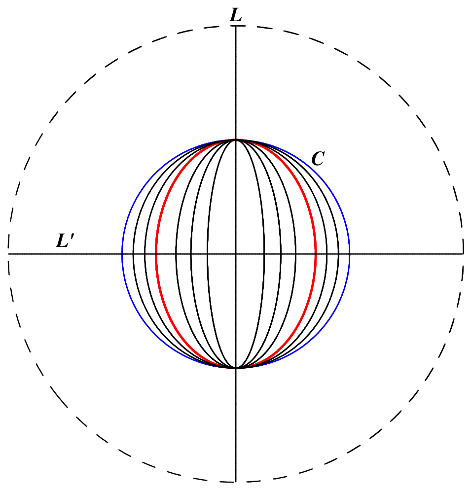
Each element of the fiber over $E_{ϵ}$ is in the closed disk bounded by the circle $E_{{ϵ}^{\prime }}\circ E_{{ϵ}^{\prime }}$, where ${ϵ}^{\prime }=\tanh {\displaystyle \frac{1}{2}}\kappa$. The fiber over $E_{{\displaystyle \frac{4}{5}}}$ is shown in Figure 8, with the ellipse in red, the circle in blue, and the remaining fiber elements in black.

In the fiber over $E_{ϵ}$, let $C\left(\epsilon \right)=E_{{ϵ}_1}\circ E_{{ϵ}_2}$, where $\epsilon =\tanh \left({\kappa }_2-{\kappa }_1\right)$. As with ellipses, we consider $C\left(\epsilon \right)$ and $C\left(-\epsilon \right)$ to be oppositely oriented fiber elements and define $\epsilon$ to be the (oriented) eccentricity of $C\left(\epsilon \right)$. The fiber elements are parameterized by ${\epsilon }_t=\tanh \left(\kappa +t\right)$, with $t=-2{\kappa }_1$ because ${\kappa }_1+{\kappa }_2=\kappa$. Define $C\left({\epsilon }_{t_1}\right)+C\left({\epsilon }_{t_2}\right):=C\left({\epsilon }_t\right)$, where ${\epsilon }_t=\tanh \left(2\kappa +t_1+t_2\right)$. Then the fiber is a group isomorphic to $G_0\left(L\right)$. The identity element is the bounding circle $C\left(0\right)$. The fiber is preserved by $G_0\left(L\right)$ with the action defined by $g·C\left({\epsilon }_t\right):=C\left({\epsilon }_t\right)+C\left(\gamma \right)$, where g is represented by the ellipse $E_{\gamma }$. Further, $G_0\left(L\right)$ acts transitively on the set of fibers, with g sending the fiber over $E_{ϵ}$ to the fiber over $\pi \left(E_{ϵ}\circ E_{\gamma }\right)$.

Proposition 5.

The conics in category C4 are partitioned into fibers over the ellipses. The group $G_0\left(L\right)$ acts transitively on the fibers, and each fiber is a group isomorphic to $G_0\left(L\right)$.

The conics can also be partitioned by eccentricity. Define the $\epsilon$-section by selecting the (unique) element in each fiber with eccentricity $\epsilon$. Then $E_{\epsilon }$ is the unique ellipse in the section. For $\epsilon ={\displaystyle \frac{1}{2}}$, the ellipse is shown in red Figure 9, with the other section elements in black.

For $ϵ\ne 0$, the fiber over a hyperbola ${\left(E_{ϵ}\right)}_{‡}$ is the split inversion of the fiber over $E_{ϵ}$. Figure 10 shows the fiber over ${\left(E_{{\displaystyle \frac{4}{5}}}\right)}_{‡}$, with the hyperbola in red. The elements are bounded by ${\left(E_{{\displaystyle \frac{1}{2}}}\circ E_{{\displaystyle \frac{1}{2}}}\right)}_{‡}$, shown in blue, which is in category C9B by Corollary 4. In this example, the distance between these ultra-parallel lines is $\ln 2$ (see Remark 5).

The KC-convex hyperbolas in the fiber over ${\left(E_{ϵ}\right)}_{‡}$ can be assigned eccentricities greater than 1 in accordance with Equation (16) and consistent with the fiber over $E_{ϵ}$. A section for a given eccentricity would then be the split inversion of an $\epsilon$-section of KC-ellipses.

11. Conclusions

In Jakob Steiner’s preface to [2] he states

Here the main thing is neither the synthetic nor the analytic method, but the discovery of the mutual dependence of the figures and of the way in which their properties are carried over from the simpler to the more complex ones.

The source of this quote has been the inspiration for the constructions in this article. These constructions were obtained intrinsically, within conformal models of the hyperbolic plane, from the incidence properties of ${\mathbb{H}}^2$ and the action of its collineation group. This is in the spirit of Steiner’s construction of conics. We used elliptic curve addition on the orthogonal trajectories of the central Steiner conics to generate all central conics, which in turn imposed a group structure on the Steiner conics themselves.

The underlying symmetries of the central conics made these constructions possible. Though we previously classified all Steiner conics in ${\mathbb{H}}^2$, we are not aware of analogous results for the categories of non-central conics. Many of these are of a so-called parabolic type, but there does not appear to be an inversive representation of the Steiner parabolas for which their orthogonal trajectories have a simple addition structure. Also, the determination of the Steiner parabolas in [1] is rather complicated, and their locus characterizations involve distance not to a line but to a rather specific equidistant curve. (The KC-parabolas themselves are quite varied due to the nature of their absolute points.) Perhaps this work will encourage further investigation.