
The Multiple Utility of Kelvin’s Inversion


Abstract
1. Introduction
2. Kelvin’s Inversion
2.1. Definition and Properties of Kelvin’s Inversion
Comment: Kelvin’s inversion is generally defined in [4], but since this transformation does not depend on in this paper, only the cases where and will be studied.
- (a)
- Kelvin’s inversion is its own inverse, which means that
- (b)
- If is a constant, it stands that
- (c)
- The unit vectors of are the same, i.e.,
- (a)
- Then,and therefore,
- (b)
- Moreover,
- (c)
- Finally,
- It is a radial transformation (i.e., the transformation is based on its distance from a point);
- It is a non-linear transformation since
- It acts on every direction as an one-to-one inversion;
- It maps points near to the center of the sphere to infinity and vice versa;
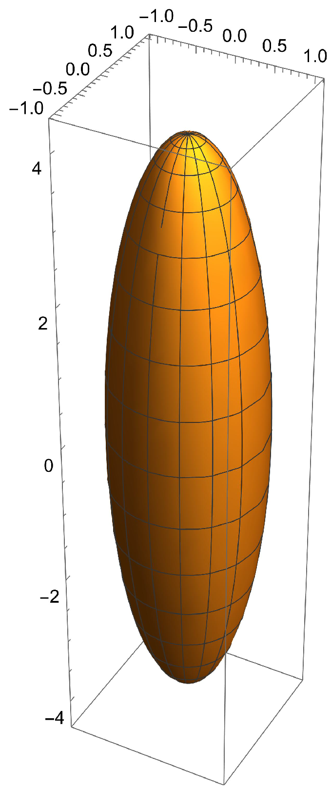
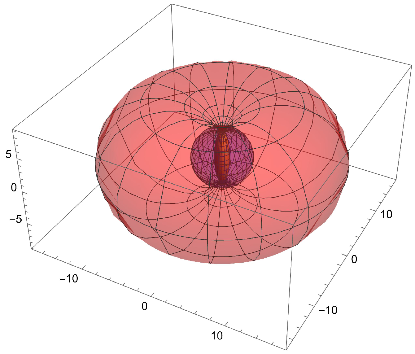
- It maps a point near and inside the sphere of inversion to a point near the sphere of inversion but outside of it and vice versa (Figure 1).

- (a)
- Preserves the angle between two vectors;
- (b)
- Inverts spheres to spheres (as we consider a sphere with infinity radius, i.e., a plane);
- (c)
- Inverts planes to spheres passing through the center of inversion and vice versa.
- (a)
- Let be the angles between the vectors and respectively. Therefore,deriving that since
- (b)
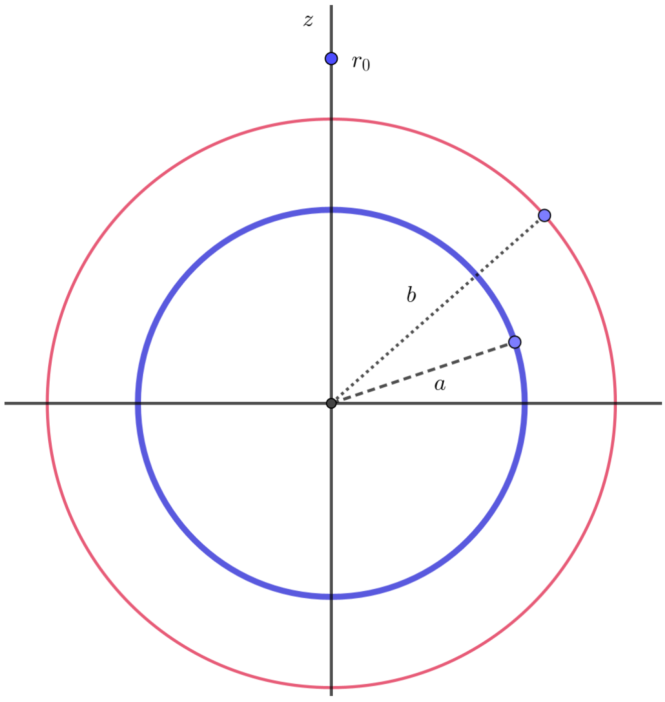
- If is a vector corresponding to a sphere of radius thenreflecting the fact that the inverted vector corresponds to a sphere of radiusThe proof of the reverse proposition is similar.
- (c)
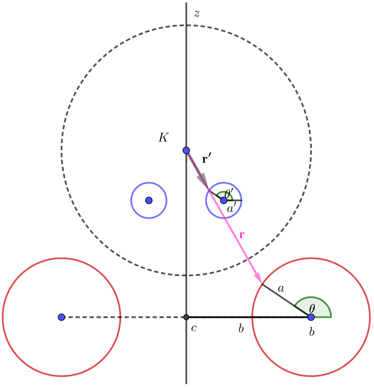
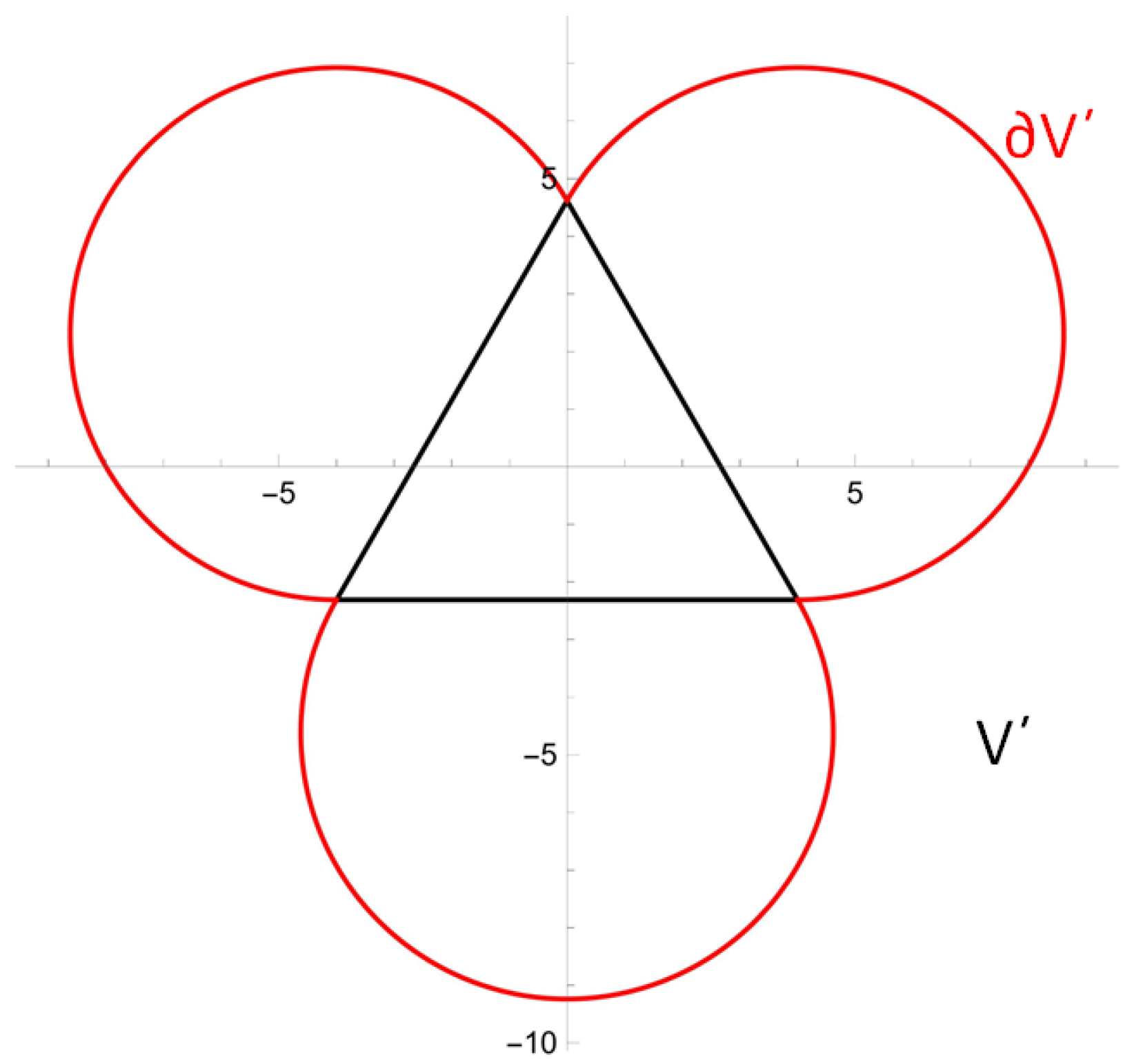
- Let with be the equation of the sphere passing through the point Then, using spherical coordinates [26], we deriveandTherefore,which proves that the image of vector belongs to the plane with equation The proof of the inverse proposition is similar (Figure 2).
2.2. Kelvin’s Inversion in Coordinate Systems
2.3. Kelvin’s Inversion in Potential Theory
- If function is a harmonic function in then function is a harmonic function in
- If function is a smooth enough biharmonic function in then function is a biharmonic function in
2.4. Kelvin’s Inversion in Stokes Flow
- If is a smooth enough stream function in then is a stream function in
- If is a smooth enough bistream function in then is a bistream function in
3. Applications
3.1. Scattering
3.1.1. Capacity and Rayleigh Scattering
3.1.2. Low-Frequency Acoustic Scattering
3.2. Electrostaticity
3.2.1. Conducting Torus
3.2.2. Dielectric-Coated Conducting Sphere
3.2.3. Multipoles
3.3. Thermoelasticity
3.4. Potential Theory
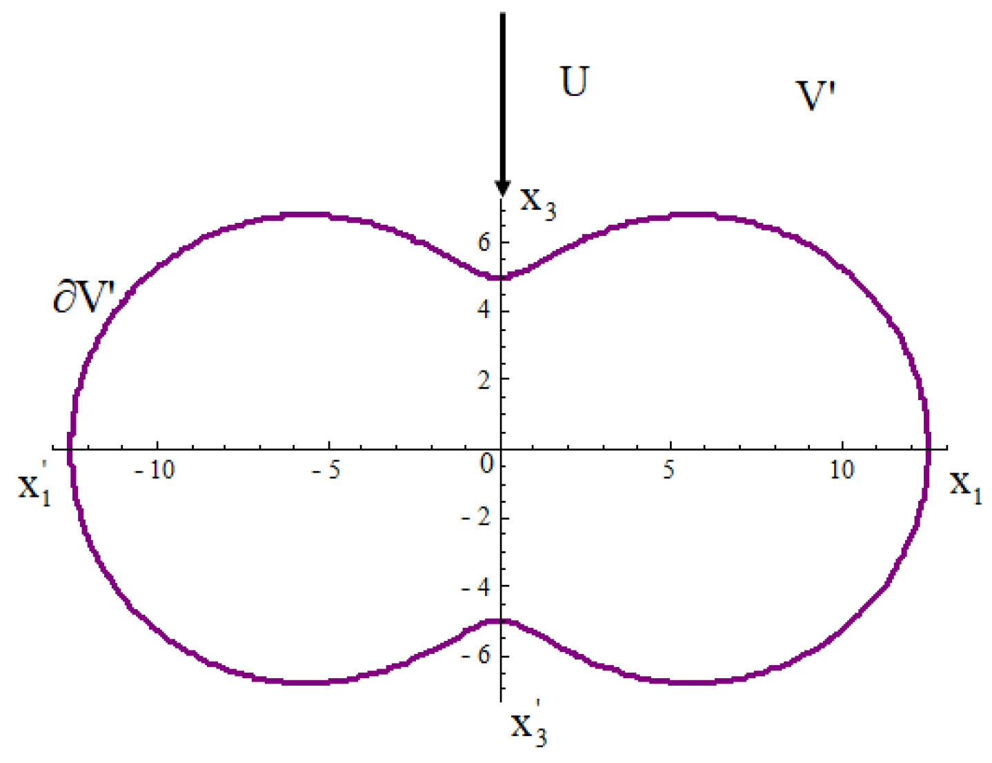
3.5. Bioengineering
4. Discussion
Funding
Data Availability Statement
Conflicts of Interest
Abbreviations
| PDE | Partial Differential Equation |
| BVP | Boundary Value Problem |
| BC | Boundary Condition |
| RBC | Red Blood Cell |
References
- Axler, S.; Bourdon, P.; Ramey, W. Harmonic Function Theory; Springer: Berlin/Heidelberg, Germany, 1992. [Google Scholar]
- Thomson, W. Ex trait d’UN letterer DE M. William Thomson (reported by A. M. Liouville). J. Math. Pure Appl. 1845, 10, 364–367. [Google Scholar]
- Green, G. An Essay on the Application of Mathematical Analysis to the Theories of Electricity and Magnetism; Private Publication, Nottingham, UK, 1928. Also in Mathematical Papers of the Late George Green; Ferrers, N.M., Ed.; Macmillan: London, UK, 1871. [Google Scholar]
- Thomson, W. Papers on Electrostatics and Magnetism; MacMillan: London, UK, 1882. [Google Scholar]
- Thomson, W. Ex traits DE Dex letterers addressees A. M. Liouville. J. Math. Pure Appl. 1847, 10, 256–264. [Google Scholar]
- Dassios, G. The Kelvin transformation in potential theory and Stokes flow. IMA J. Appl. Math. 2009, 74, 427–438. [Google Scholar]
- Dassios, G.; Kleinman, R. On the Capacity and Reyleigh Scattering for a Class of Non–Convex Bodies. J. Mech. Appl. Math. 1989, 42, 467–475. [Google Scholar]
- Gintides, D.; Kyriakie, K. Low-Frequency acoustic scattering by a hard inverse-prolate spheroid. J. Mech. Appl. Math. 1992, 45, 231–244. [Google Scholar]
- Baganis, G.; Hadjinicolaou, M. Analytic Solution of an Exterior Dirichlet Problem in a Non-Convex Domain. IMA J. Appl. Math. 2009, 74, 668–684. [Google Scholar]
- Baganis, G.; Hadjinicolaou, M. Analytic Solution of an Exterior Neumann Problem in a Non-Convex Domain. Math. Methods Appl. Sci. 2010, 33, 2067–2075. [Google Scholar]
- Fokas, A.S. Two-dimensional linear partial differential equations in a convex polygon. Proc. R. Soc. A 2001, 457, 371–393. [Google Scholar]
- Fokas, A.S.; Kapaev, A.A. Riemann–Hilbert approach to the Laplace equation. J. Math. Anal. Appl. 2000, 251, 770–804. [Google Scholar]
- Pyati, P.V. Kelvin transformation for a dielectric-coated conducting sphere. Radio Sci. 1993, 28, 1105–1110. [Google Scholar]
- Amaral, G.P.L.R.; Ventura, S.O.; Lemos, A.N. Kelvin transformation and inverse multipoles in electrostatistics. Eur. J. Phys. IOP Publ. 2017, 38, 025206. [Google Scholar] [CrossRef]
- Cade, R. The Kelvin transformation of a torus. J. Appl. Phys. 1978, 49, 5722–5727. [Google Scholar]
- Chao, K.C.; Wu, H.C.; Ting, K. The inversion and Kelvin’s transformation in plane thermoelasticity with circular or straight boundaries. J. Mech. 2018, 34, 617–627. [Google Scholar]
- Dassios, G.; Hadjinicolaou, M.; Protopapas, E. Blood Plasma Flow Past a Red Blood Cell: Mathematical Modelling and Analytical Treatment. Math. Methods Appl. Sci. 2012, 35, 1547–1563. [Google Scholar]
- Hadjinicolaou, M.; Protopapas, E. Eigenfunction expansions for the Stokes flow operators in the inverted oblate coordinate system. Math. Probl. Eng. 2016, 2016, 9049131. [Google Scholar] [CrossRef]
- Simunkova, M. On Kelvin type transformation for Weinstein operator. Comment. Math. Univ. Carolin. 2001, 42, 99–109. [Google Scholar]
- Monti, R.; Morbidelli, D. Kelvin transform for Grushin operators and critical semilinear equation. Duke Math. J. 2006, 131, 167–202. [Google Scholar]
- Clerc, L.-J. Kelvin transformation and multi-harmonic polynomials. Acta Math. 2000, 185, 81–99. [Google Scholar]
- Michalik, K.; Ryznar, M. Kelvin transform for a-harmonic functions in regular domain. Demonstr. Math. 2012, 45, 361–376. [Google Scholar]
- Wei, Y.; Zhou, X. Pohozaev identities and Kelvin transformation of semilinear Grushin equation. arXiv 2024, arXiv:2404.11991v1. [Google Scholar]
- Koranyi, A. Kelvin transforms and harmonic polynomials on the Heisenberg group. J. Funct. Anal. 1982, 49, 177–185. [Google Scholar]
- Nabizadeh, S.M.; Ramamoorthi, R.; Chern, A. Kelvin transformations for simulations on infinite domains. ACM Trans. Graph. 2021, 40, 97. [Google Scholar]
- Moon, P.; Spencer, D.E. Field Theory Handbook; Springer: Berlin/Heidelberg, Germany, 1961. [Google Scholar]
- Hadjinicolaou, M.; Protopapas, E. Necessary and sufficient conditions for the separability and the R-separability of the irrotational Stokes equation. J. Appl. Math. Phys. 2020, 8, 2379–2401. [Google Scholar] [CrossRef]
- Liouville, J. Extension au cas des trois dimensions de la question du trace geographique. In Note VI. Application de l’Analyse a la Geometrie; Monge, G., Ed.; Bachelier, Imprimeur-Libraire: Paris, France, 1850; pp. 609–616. [Google Scholar]
- Stokes, G.G. On the theories of the internal friction of fluids on the motion of pendulums. Trans. Camb. Philos. Soc. 1849, 9, 287–319. [Google Scholar]
- Stokes, G.G. On the Effect of the Internal Friction of Fluids on the Motion of Pendulums. Trans. Camb. Philos. Soc. 1851, 8, 8–106. [Google Scholar]
- Happel, J.; Brenner, H. Low Reynolds Number Hydrodynamics; Kluwer Academic Publishers: Dordrecht, The Netherlands, 1991. [Google Scholar]
- Jeans, J. The Mathematical Theory of Electricity and Magnetism; Cambridge University Press: New York, NY, USA, 1960; Chapter VIII. [Google Scholar]
- Smythe, W.R. Static and Dynamic Electricity; Hemisphere: New York, NY, USA, 1989; Chapter V. [Google Scholar]
- Weiss, P. Applications of Kelvin’s transformation in electricity, magnetism and hydrodymanics. Proc. Camb. Philos. Soc. 1944, 40, 200–214. [Google Scholar]
- Wang, X.Z.; Guo, R.D. Special Functions; World Scientific: Singapore, 1989. [Google Scholar]
- Dassios, G.; Fokas, A.S. The basic elliptic equations in an equilateral triangle. Proc. Soc. A 2005, 461, 2721–2748. [Google Scholar]
- Hadjinicolaou, M.; Protopapas, E. Non-Convex Particle-in-Cell Model for the Mathematical Study of the Microscopic Blood Flow. Mathematics 2023, 11, 2156. [Google Scholar] [CrossRef]
- Ebenfelt, P.; Khavinson, D. On point to point reflection of harmonic functions across real-analytic hypersurfaces in Rn. J. Anal. Math. 1996, 68, 145–182. [Google Scholar] [CrossRef]
- Khavinson, D.; Lundberg, E. Linear Holomorphic Partial Differential Equations and Classical Potential Theory; American Mathematical Society: Providence, RI, USA, 2018. [Google Scholar]


Disclaimer/Publisher’s Note: The statements, opinions and data contained in all publications are solely those of the individual author(s) and contributor(s) and not of MDPI and/or the editor(s). MDPI and/or the editor(s) disclaim responsibility for any injury to people or property resulting from any ideas, methods, instructions or products referred to in the content. |
© 2025 by the author. Licensee MDPI, Basel, Switzerland. This article is an open access article distributed under the terms and conditions of the Creative Commons Attribution (CC BY) license (https://creativecommons.org/licenses/by/4.0/).
Share and Cite
Protopapas, E. The Multiple Utility of Kelvin’s Inversion. Geometry 2025, 2, 11. https://doi.org/10.3390/geometry2030011
Protopapas E. The Multiple Utility of Kelvin’s Inversion. Geometry. 2025; 2(3):11. https://doi.org/10.3390/geometry2030011
Chicago/Turabian StyleProtopapas, Eleftherios. 2025. "The Multiple Utility of Kelvin’s Inversion" Geometry 2, no. 3: 11. https://doi.org/10.3390/geometry2030011
APA StyleProtopapas, E. (2025). The Multiple Utility of Kelvin’s Inversion. Geometry, 2(3), 11. https://doi.org/10.3390/geometry2030011