Article

Uses of the Popov Stability Criterion for Analyzing Global Asymptotic Stability in Power System Dynamic Models

1
The Andrew and Erna Viterbi Faculty of Electrical and Computer Engineering, Technion—Israel Institute of Technology, Haifa 3200003, Israel
2
Department of Software Science, Tallinn University of Technology, Akadeemia tee 15a, 12618 Tallinn, Estonia
3
Advanced Energy Industries, Caesarea 4809234, Israel
*
Author to whom correspondence should be addressed.
Energy Storage Appl. 2024, 1(1), 54-72; https://doi.org/10.3390/esa1010005
Submission received: 30 September 2024 / Revised: 1 December 2024 / Accepted: 20 December 2024 / Published: 23 December 2024

Abstract

:
Stability studies remain a crucial aspect of power systems dynamic analysis, and are typically explored in three main categories: numerical methods, linearization techniques, or direct methods, which utilize Lyapunov energy functions. This paper belongs to the third category, and highlights the usefulness of the Popov stability criterion in the analysis of nonlinear power system models. The main advantage of this criterion is that it provides conditions for global asymptotic stability of an equilibrium point, for a nonlinear dynamic system. We show a general method to apply this stability criterion, and examine its uses in several specific applications and case-studies. The results are demonstrated by analyzing the stability of a system that includes a grid-connected storage device and a renewable energy source.

1. Introduction

Stability studies remain a crucial aspect of power systems dynamic analysis. Despite the fact that stability problems in power systems have been researched for a very long time [1,2,3], the increasing penetration of renewable energy sources, and the rapid evolution of technology, have given rise to more intricate and complex system dynamics, which necessitates a deeper and wider perspective [4,5,6]. The core of the problem lies in the fact that renewable energy sources, such as wind and solar, are inherently intermittent and often unpredictable due to their dependence on environmental conditions. This variability introduces challenges in maintaining a stable frequency within the power grid, a parameter that is crucial for the reliable operation of electrical power systems. Frequency stability is maintained by balancing the supply and demand of power within the grid. However, the intermittent nature of renewable sources can lead to significant deviations if not properly managed. These deviations can cause a range of issues, from minor inefficiencies to severe system failures, including blackouts or damage to sensitive infrastructure. Energy storage systems (ESSs) have emerged as a vital solution to address these challenges, providing the necessary flexibility to absorb or release energy in response to fluctuations in supply and demand [7,8,9]. By quickly adjusting their output, ESSs can help smooth out the variability in renewable energy generation, thereby stabilizing the frequency of the grid.
Many works in the recent literature study stability problems in power systems, using different approaches. This vast field of research can be divided roughly to three main approaches: numerical analysis [10,11,12], linearization-based techniques [13,14,15,16], and direct methods—which utilize at their core various Lyapunov energy functions [17,18,19]. Considering the direct methods, one may examine, for instance, the work of [20], which presents a theoretical foundation of direct methods for both network-reduction and network-preserving power system models. The authors suggest a systematic procedure for constructing energy functions for both network-reduction and network-preserving power system models, utilizing the “boundary of stability region-based controlling unstable equilibrium point” (or BCU) method. A practical demonstration of the proposed method for online transient stability assessments of two power system models is outlined. Moreover, the paper in [21] introduces a novel framework for constructing the Region of Attraction (ROA) of a power system centered around a stable equilibrium by using stable-state trajectories of the system dynamics. The proposed method leverages a Lyapunov function along with the Gaussian process approach. In addition, a sampling algorithm is designed to reconcile the tradeoffs between attaining a larger ROA, and obtaining suitable confidence levels. The writers conduct various simulations and experiments to validate their approach, by computing the ROA of standard IEEE case-study systems. It is demonstrated that the proposed approach can significantly enlarge the estimated ROA compared to previous works.
As described above, a large number of works utilize linearization techniques to study the stability of power systems. Due to the vast amount of research in this field, we naturally review only several representative papers. For example, the study in [22] investigates the application of a multi-variable nonlinear controller for generators. The proposed controller is based on linearization, and its main goal is to improve the transient stability and voltage regulation under post-fault conditions. Simulation results show the improvement in swing stability and system damping under large disturbances, as well as robust terminal voltage regulation. To continue this line of thinking, researchers in [23] offer a new framework to study integration methods for power systems impacted by delays. They use matrix-pencil theory for numerical stability analysis and accuracy analysis. The proposed approach covers all implicit Runge–Kutta methods for time-delay systems. The authors illustrate the idea through simulations on the IEEE 14-bus system, and consider three examples of implicit integration methods, such as “Backward Euler”, “trapezoidal”, and “2-s Radau IIA”.
There are also works that combine the different methods, and some of them examine inverter-dominated grids. For example, ref. [24] addresses the reduction of inertia in the system due to increases in the share of inverter-based generation. Specifically, it focuses on power system instability caused in low-inertia systems when there is a power imbalance, as in the case of a system split. In the paper, they analyze frequency stability during system split within a test system. In their numerical results, they present and compare different modeling approaches. The study in [25] focuses on imbalances present in a microgrid with renewable energy sources. The authors propose a new algorithmic approach that simulates the dynamic behavior of the microgrid, under grid connected and autonomous operation. The simulation accuracy is illustrated by several case studies. Consequently, in article [26], the authors present a new and extended framework for stability studies. They discuss the properties of inverter-based resources, focusing specifically on grid-forming and grid-following topologies. The authors also compare these models to synchronous generators in terms of synchronization, inertia, and voltage control. Finally, several future research directions are proposed.
Moreover, there are several works focusing on hybrid renewable energy systems. For instance, ref. [27] reviews hybrid renewable energy systems (HRES) that use renewable sources like solar and wind. The paper discusses the design of these systems, including the configuration of components and power converters. The paper also focuses on control strategies for system stability, power quality, and load sharing, highlighting recent advancements in HRES design and control, and discussing future developments to increase the use of renewable energy. Another perspective is given in [28]. The paper discusses the potential of offshore wind energy to address electricity shortages and its advantages in comparison to onshore wind energy. To decrease the risks of instability, hybrid offshore solar and wind farms are proposed. More specifically, the paper focuses on the impact of large-scale offshore hybrid farms (OHFs) on power system stability. It proposes using high-voltage direct current technology with voltage source converters to connect OHFs to the main grid. The paper presents a method for optimal sizing of OHFs to ensure grid stability, and uses the IEEE New-England 10-machine 39-bus test system for simulation and analysis.
As seen in the literature review above, there exist three central approaches to analyzing the stability of power system dynamic models, namely, numeric simulations, linearization techniques, and direct methods, which utilize a variety of Lyapunov functions. In this paper, we continue the line of thinking represented by this last approach, and propose a new criterion for finding global stability properties of equilibrium points in nonlinear power system models. Our approach is based on the Popov stability criterion, which provides exactly this kind of information. With respect to previous works, the proposed method has the following properties:
  • With respect to linearization techniques, the proposed approach provides information on the global stability of an equilibrium point of a power system model, rather than on its local stability.
  • With respect to numerical techniques, the proposed approach provides analytical conditions, which apply generally to the type of system under study.
  • With respect to direct methods, the proposed approach provides a systematic procedure for applying the Popov stability criterion in various power system models, which has not been used before in this application, and thus enables a systematic analysis of several small-scale systems, as described in the text below.
We first present the general mathematical background, and then proceed with practical applications of this proposed approach.

2. Materials and Methods

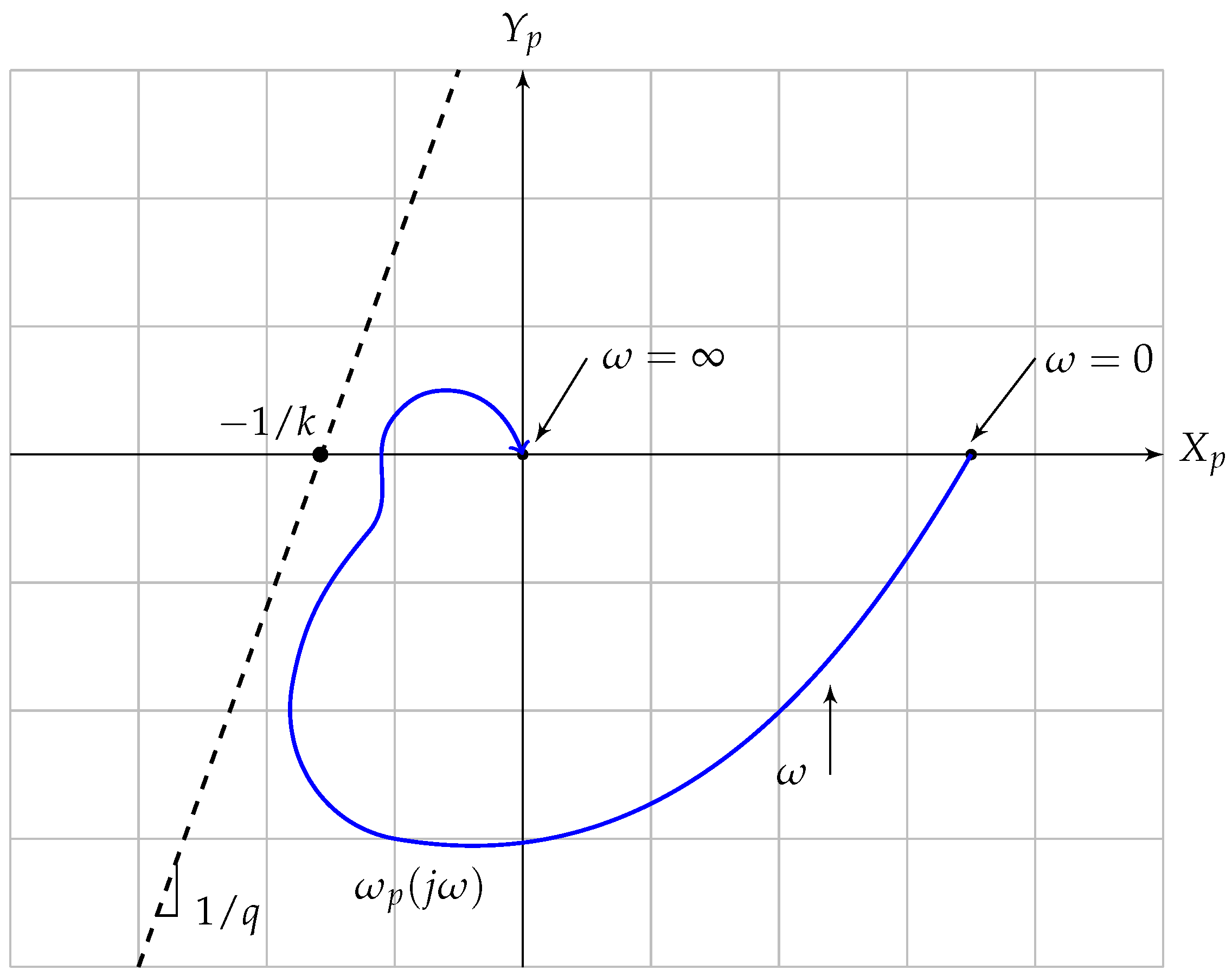
2.1. Mathematical Background—The Popov Stability Criterion

The Popov stability criterion applies to nonlinear feedback systems that include a memory-less nonlinear component. Unlike linearization techniques, this criterion provides conditions for the global asymptotic stability of an equilibrium point. Consider the following dynamic system:
x ˙ = A x b ϕ ( σ ) σ = c T x ,
where A is a constant matrix, b and c are constant vectors, and ϕ ( σ ) is a continuous function of σ that describes the nonlinearity. The following are assumed:
  • The eigenvalues of the constant matrix A are in the open left half-plane,
  • ϕ ( 0 ) = 0 ,
  • 0 < ϕ ( σ ) / σ k < , for all σ 0 , where k is a positive constant.
The system is described in Figure 1.
Popov’s stability criterion states that an equilibrium point of the dynamic system (1) is globally asymptotically stable if there exist real numbers q ,   η such that the inequality
Re { ( 1 + j ω q ) G ( j ω ) } + 1 / k η > 0 ,
holds for every real ω 0 . Defining
G ( s ) = c T ( s I A ) 1 b , X p ( ω ) = Re { G ( j ω ) } , Y p ( ω ) = ω Im { G ( j ω ) } ,
one can plot the “Popov plot”, shown in Figure 2. In this figure, if the plot is indeed in the right-half plane defined by the straight line with slope 1 / q , which intersects with the x-axis at 1 / k , then the conditions of the Popov criterion hold, and the equilibrium point of (1) is globally asymptotically stable, for every 0 < ϕ ( σ ) / σ k . We proceed by describing the implementation of this criterion in power system dynamic models.

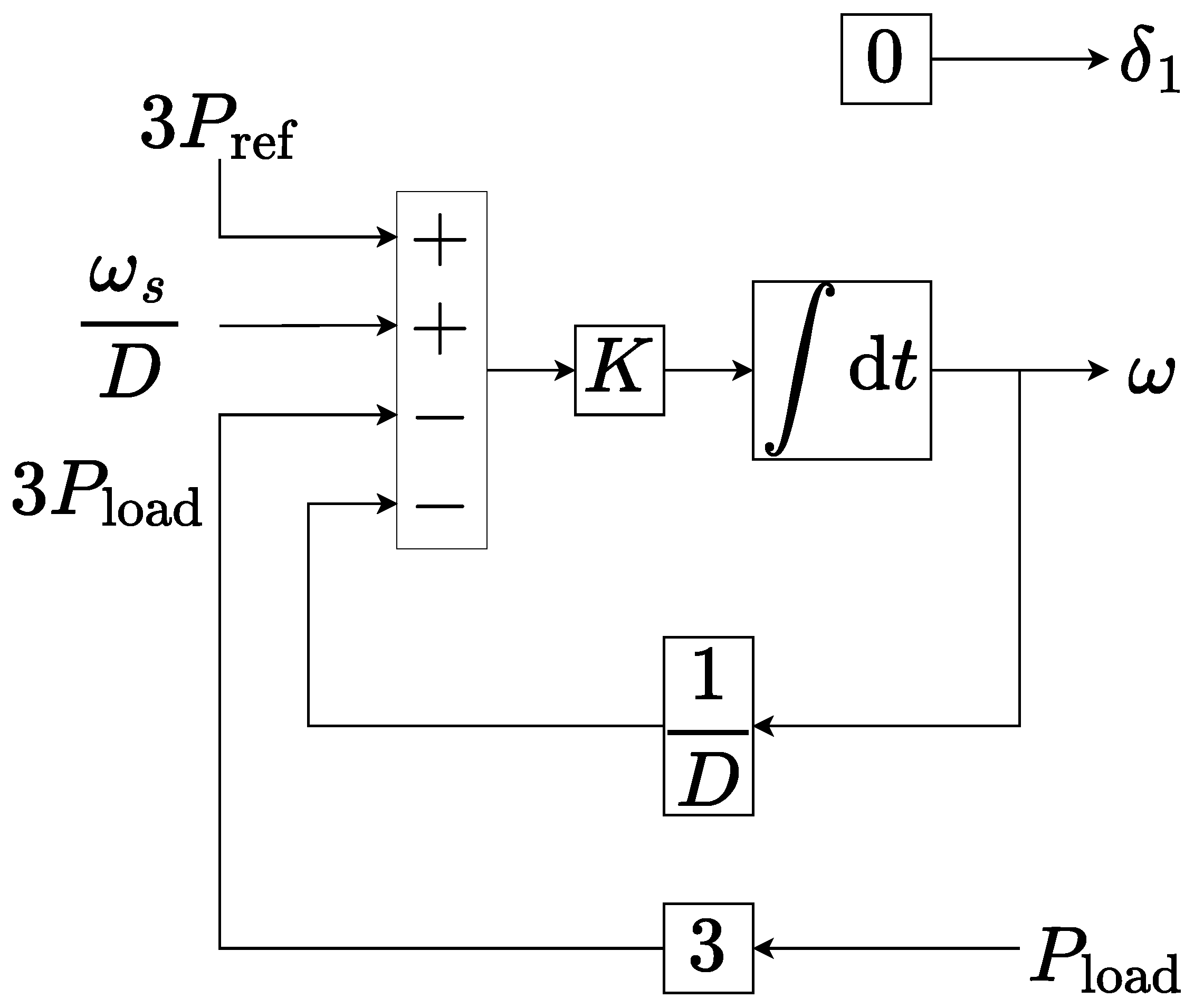
2.2. Dynamic Stability of Synchronous Generator Connected to Non-Linear Frequency Dependent Load

Consider a system consisting of a synchronous generator connected to non-linear load, as shown in Figure 3. We adopt an idealized model, in which all the power generated is transferred without loss directly to the load.
The system is described by the following differential equation:
H d d t ω + D · ( ω ω s ) = P ref P load ( ω ) ,
where H > 0 represents the moment of inertia of the rotor, ω is the electrical frequency of the rotor, D > 0 stands for the damping coefficient, and without loss of generality, P ref = P load ( ω s ) represents the reference power, where ω s is the nominal angular velocity. The power consumed by the load is a general non-linear function of the electrical angular frequency P load = P load ( ω ) . For the system (4), there is at least one equilibrium point located at ω = ω s . It is trivial to verify that linearizing (4) in a small neighborhood of the equilibrium point ω = ω s leads to
H d d t ω ^ = D + d P load d ω ω = ω s · ω ^ ,
where ω ^ = ω ω s , so the equilibrium point ω = ω s is locally asymptotically stable if
D < d P load d ω ω = ω s .
We extend here this well-known result by providing a sufficient condition for the global asymptotic stability of the equilibrium ω = ω s ; that is, we provide a condition under which any trajectory ω ( t ) of (4) converges to ω s as t , from any initial point. Our main claim consists of two parts, and it is the following:
Theorem 1.
Consider the dynamic system (4) with a load profile P load ( ω ) , which is generally a nonlinear but continuous function of ω. If there exists a constant k such that
D < P load ( ω ) P ref ω ω s k
for all ω ω s , then the equilibrium point ω = ω s is the only equilibrium point of (4), and it is globally asymptotically stable.
In addition, if P load ( ω ) is differentiable at ω s , and D > d P load / d ω ω = ω s , or equivalently,
D > lim ω ω s P load ( ω ) P ref ω ω s ,
then the equilibrium ω = ω s is unstable.
Proof. 
We start by proving the second part of the theorem, the instability condition given in (8). Examine the linearized system described in (5). It is clear that this system has one real pole with value D d d ω P load ( ω ) ω = ω s . A strictly positive pole means that the equilibrium point ω s is unstable; thus, the system is unstable if
D d d ω P load ( ω ) ω = ω s > 0 ,
which is the same as
d d ω P load ( ω ) ω = ω s < D ,
and by definition of the derivative, we obtain
d d ω P load ( ω ) ω = ω s = lim ω 0 P load ( ω s + ω ) P load ( ω s ) ω .
Now, the following equivalent expression may be used:
d d ω P load ( ω ) ω = ω s = lim ω ω s P load ( ω ) P load ( ω s ) ω ω s .
Substituting (12) in (10) results in
lim ω ω s P load ( ω ) P ref ω ω s < D ,
which completes the proof for the instability condition in (8).
Now, we proceed to prove the first claim in the main theorem, the stability condition given in (7), based on Popov’s criterion. Let us define ϕ ( ω ) = P load ( ω ) P ref and ω ω ω s . Substitute these values in (4) to obtain
d d t ω = D H ω 1 H ϕ ( ω ) .
Assuming condition (7) is true, we now show that (2) holds. For the choice of x = ω ,   A = D / H ,   b = 1 / H and σ = 1 · ω , the transfer function of the system is
G ( s ) = 1 H s + D H .
Now, we shall find q R and a small and positive constant η that satisfy (2). Substitution of (15) in the right expression of (2) results in
Re { ( 1 + j ω q ) G ( j ω ) } + 1 k = 1 H ( D H ) 2 + ω 2 D H + ω 2 q + 1 k .
For the choice of ω = 0 , we can directly choose the lower bound to be η = 1 D + 1 k > 0 . Now, by analysing the “Popov plot”, we find the values of q R for which (2) holds. To plot the “Popov plot”, we rely on
X p ( s = j ω ) = Re { G ( s = j ω ) } = D ( D H ) 2 + ω 2 , Y p ( s = j ω ) = Im { G ( s = j ω ) } = 1 H ( D H ) 2 + ω 2 ω 2 .
Notice that by taking ω 0 , the resulting point on the “Popov plot” is ( H 2 D , 0 ) , and for ω , the point on the “Popov plot” is ( 0 , 1 H ) . Between these points, the transfer function is continuous and is shaped like a quarter of a circle. By the geometric interpretation of (2), it is sufficient to find a straight line, with a slope of 1 / q that intersects the x-axis at 1 / k , and is located strictly to the left of the plot of the “Popov plot” of the transfer function. In this case, it is clear that for every choice of a positive slope, the “Popov plot” of the transfer function will be strictly to the right of this straight line, in particular for the value of q = 1 . Consequently, if condition (7) holds, then there exist q R and a small positive constant η such that (2) holds, meaning that the equilibrium is globally asymptotically stable, as desired. □
The following corollary can be used to analyze the stability of a typical small power system, in which a synchronous machine is feeding a general frequency dependent impedance Z ( j ω ) .
Corollary 1.
If the load power is given by
P load ( ω ) = 3 | V | 2 Re { Z ( j ω ) } | Z ( j ω ) | 2 ,
where | V | is constant, Re { Z ( j ω ) } is bounded from above, | Z ( j ω ) | is bounded from below by a positive constant, Re { Z ( j ω ) } ,   Im { Z ( j ω ) } C 1 , and
D > 3 | V | 2 ω ω s Re { Z ( j ω s ) } | Z ( j ω s ) | 2 Re { Z ( j ω ) } | Z ( j ω ) | 2 ,
for all ω ω s , then the equilibrium point ω = ω s is the only equilibrium point of (4), and it is globally asymptotically stable.
Proof. 
To prove this statement, we show that it satisfies the conditions of Theorem 1. Substituting (18) and P ref = P load ( ω s ) in Corollary 1 results in
D > P load ( ω ) P ref ω ω s ,
which yields directly the lower bound:
D < P load ( ω ) P ref ω ω s .
Following this, using the fact that | V | is constant, Re { Z ( j ω ) } k 1 , and 0 < k 2 | Z ( j ω ) | , we proceed to determine the upper bound. Examining the expression
P load ( ω ) P ref ω ω s ,
and substituting (18) results in
3 | V | 2 Re { Z ( j ω s ) } | Z ( j ω s ) | 2 Re { Z ( j ω ) } | Z ( j ω ) | 2 ω ω s .
For ω 0 and ω , Expression (23) is well defined, and the upper and lower bounds can be calculated directly. Let us denote them by c l ,   c u , respectively. In the regions [ 0 , ω s ) and ( ω s , ) , Expression (23) is continuous; thus, there are no additional extremum points that can be found there. Finally, consider the limit
lim ω ω s Re { Z ( j ω s ) } | Z ( j ω s ) | 2 Re { Z ( j ω ) } | Z ( j ω ) | 2 1 ω ω s .
We now show that this limit exists, and is finite. That is, our goal is to prove that
lim ω ω s Re { Z ( j ω s ) } | Z ( j ω s ) | 2 Re { Z ( j ω ) } | Z ( j ω ) | 2 1 ω ω s = C .
We rely on the following assumptions presented in Theorem 1:
  • There exists k 1 such that Re { Z ( j ω ) } k 1 ,
  • There exists k 2 such that | Z ( j ω ) | k 2 ,
  • Re { Z ( j ω ) } ,   Im { Z ( j ω ) } C 1 .
Examining the limit (24) again, the application of L’Hopital’s rule results in
lim ω ω s d d ω Re { Z ( j ω ) } | Z ( j ω ) | 2 d d ω ( ω ω s ) = lim ω ω s d d ω Re { Z ( j ω ) } | Z ( j ω ) | 2 Re { Z ( j ω ) } d d ω | Z ( j ω ) | 2 | Z ( j ω ) | 4 .
Since Re { Z ( j ω ) } ,   Im { Z ( j ω ) } C 1 , we have that | Z ( j ω ) | = Re { Z ( j ω ) } 2 + Im { Z ( j ω ) } 2 C 1 . Hence, the following limits are well defined:
  • lim ω ω s d d ω Re { Z ( j ω ) } = c 1 ,
  • lim ω ω s | Z ( j ω ) | 2 = c 2 ,
  • lim ω ω s Re { Z ( j ω ) } = c 3 ,
  • lim ω ω s d d ω | Z ( j ω ) | 2 = c 4 .
Therefore, the original limit we are interested in is equal to
c 1 c 2 c 3 c 4 c 2 4 C .
Note that, depending on the system’s parameters, it is possible to get C > 0 or C < 0 . In each case, the value of C is a candidate for the upper or lower limit, respectively. w.l.o.g., assuming C > 0 , we deduce it is a candidate for the upper bound. Consequently, (22) is bounded by
D < P load ( ω ) P ref ω ω s k ,
where k = max { c u , C } and D = c l . Thereby, the conditions of Theorem 1 hold in this unique case, meaning that ω = ω s is indeed the only equilibrium point of (4), and it is globally asymptotically stable. □

2.3. Synchronous Machine Driving Resistive–Inductive Load

In this case-study, we analyze a system in which the nonlinear load has resistive–inductive behavior. The main claim used for the analysis is Corollary 1. Our aim is to find the minimal value of D which bounds from above the expression (19), which is derived from the active power of the system. We consider a general load model, of which the resistance and inductance are given by R ,   L , respectively, and the voltage is V. The nominal power of the synchronous machine is again P ref and the nominal frequency is ω s . The values of the parameters may vary depending on the scale of the system, as will be presented in the numeric results section. The active power of the load is given by
P load = 3 | V | 2 · R R 2 + ( ω L ) 2 .
Examine the expression
P load P ref ω ω s .
Substitution of (29) in (30) leads to
3 | V | 2 ω ω s R R 2 + ( ω s L ) 2 R R 2 + ( ω L ) 2 .
Re-writing this equation results in
1 ω ω s · ω 2 ω s 2 ( R 2 + ω s 2 L 2 ) · ( R 2 + ω 2 L 2 ) · 3 | V | 2 R L 2 ,
or, alternatively,
ω + ω s R 2 + ω 2 L 2 · 3 | V | 2 R L 2 R 2 + ω s 2 L 2 .
Next, we aim to find the minimal value that bounds (33) from above. For this purpose, notice that the expression given in (33) consists of continuous functions of ω . Hence, the derivative may be calculated directly and is given by
3 | V | 2 R R 2 + ω s 2 L 2 · ω 2 2 ω s ω + R L 2 ω 2 + R L 2 2 ,
whose critical points are
r 1 , 2 = ω s ± ω s 2 + R L 2 .
Since ω > 0 , the only valid root is r 2 , so to analyze (34), we examine its behavior close to the critical point r 2 . Given that 3 | V | 2 R R 2 + ω s 2 L 2 > 0 and ω 2 + R L 2 2 > 0 , it is sufficient to look at the sign of the following expression:
ω 2 2 ω s ω + R L 2 .
When ω r 2 , the derivative (34) is negative. This may be seen directly by looking at ω = r 2 ϵ where ϵ is a small strictly positive constant such that r 2 ϵ > 0 . In this case, the expression (36), which determines the sign of the derivative, is of the following form:
r 2 ϵ 2 2 ω s r 2 ϵ + R L 2 .
Re-arranging the terms results in
r 2 2 2 ω s r 2 + R L 2 + 2 · r 2 · ϵ ϵ 2 + 2 ω s ϵ .
For the simple choice of ϵ = r 2 , Expression (38) is positive, meaning the function increases on the interval ( , r 2 ] . In the same manner, it may be shown that when ω r 2 + , Expression (34) is negative, meaning that r 2 is a maximum point. Consequently, the upper bound may be defined as
D = ω s 2 + ( R L ) 2 R 2 + ω s + ω s 2 + ( R L ) 2 2 · L 2 · 3 | V | 2 R L 2 R 2 + ω s 2 L 2 .
This results in a strict upper bound for the expression given in (33). Indeed, the condition given in (19) holds; therefore, ω s is the only global asymptotic equilibrium point of the given system, as desired, and a simplified expression is
D = ω s 2 + ( R L ) 2 R L 2 + ω s + ω s 2 + ( R L ) 2 2 · 3 | V | 2 R R 2 + ω s 2 L 2 .
Notice that the active power at the operating point is given by P * = 3 | V | 2 R R 2 + ω s 2 L 2 and the reactive power at the operating point is defined as Q * = 3 | V | 2 ω s L R 2 + ω s 2 L 2 . We therefore have R L = ω S · P * Q * . Substituting these terms in (40) produces
D = ω s 2 + ω s 2 · ( P * Q * ) 2 ω s 2 · P * Q * 2 + ω s + ω s 2 + ω s 2 · ( P * Q * ) 2 2 · P * ,
which is the same as
D = 1 + ( P * Q * ) 2 P * Q * 2 + 1 + 1 + ( P * Q * ) 2 2 · P * ω s .
Re-arranging the terms in the expression above yields
D = 1 + ( P * Q * ) 2 P * Q * 2 + 1 2 1 + ( P * Q * ) 2 + 1 + ( P * Q * ) 2 · P * ω s ,
or
D = 1 + ( P * Q * ) 2 P * Q * 2 + 1 1 + ( P * Q * ) 2 · P * 2 ω s ,
which may be written as
D = 1 P * Q * 2 + 1 1 · P * 2 ω s ,
thereby leading to
D = Q P * + Q * 2 Q · P * 2 ω s .
In conclusion, using the fact that | S | 2 = P 2 + Q 2 , the bound on D may be presented in the following way:
D = Q | S | Q · P * 2 ω s .

2.4. Synchronous Machine Driving a Lossless Synchronous Motor with a Quasi-Linear Mechanical Load
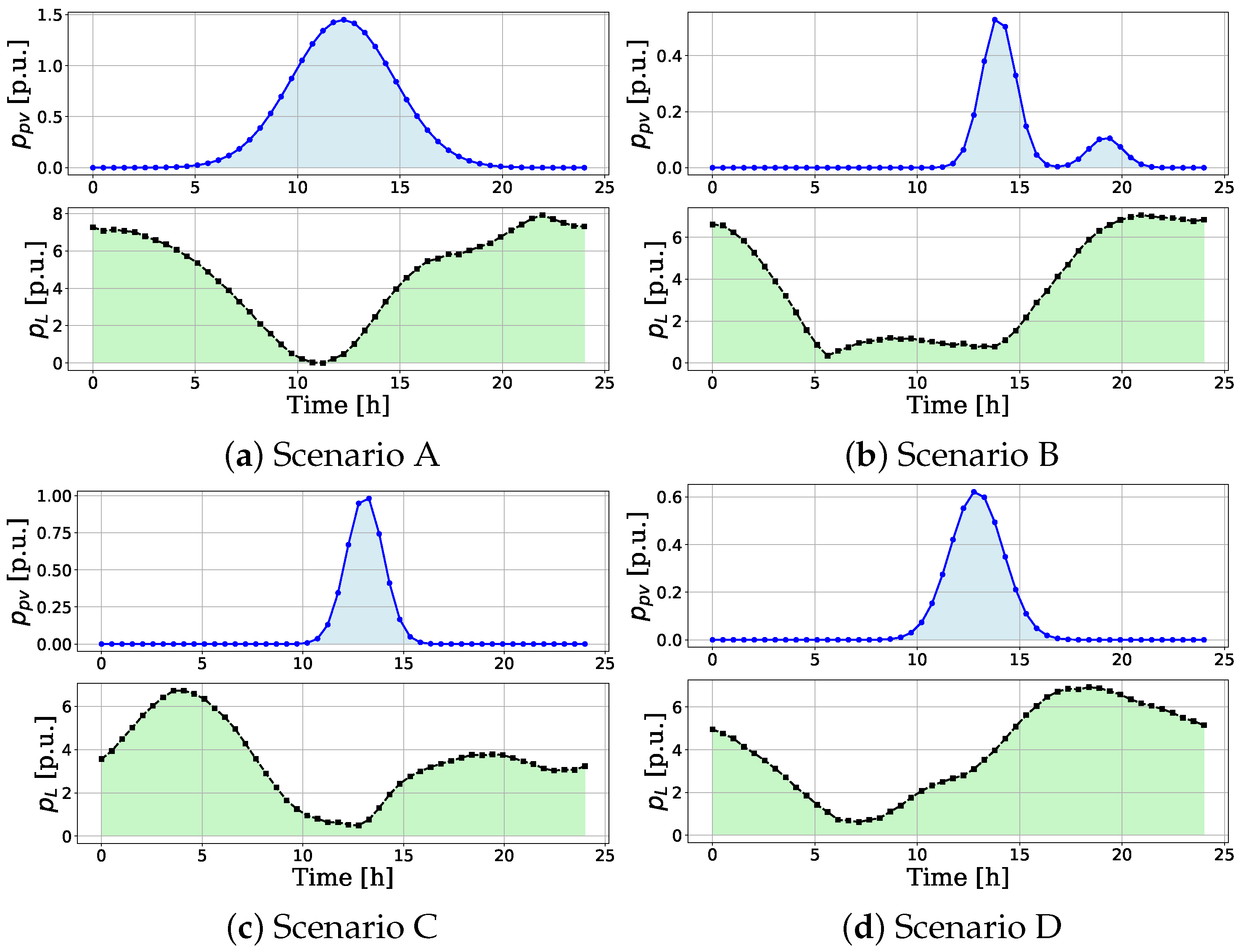
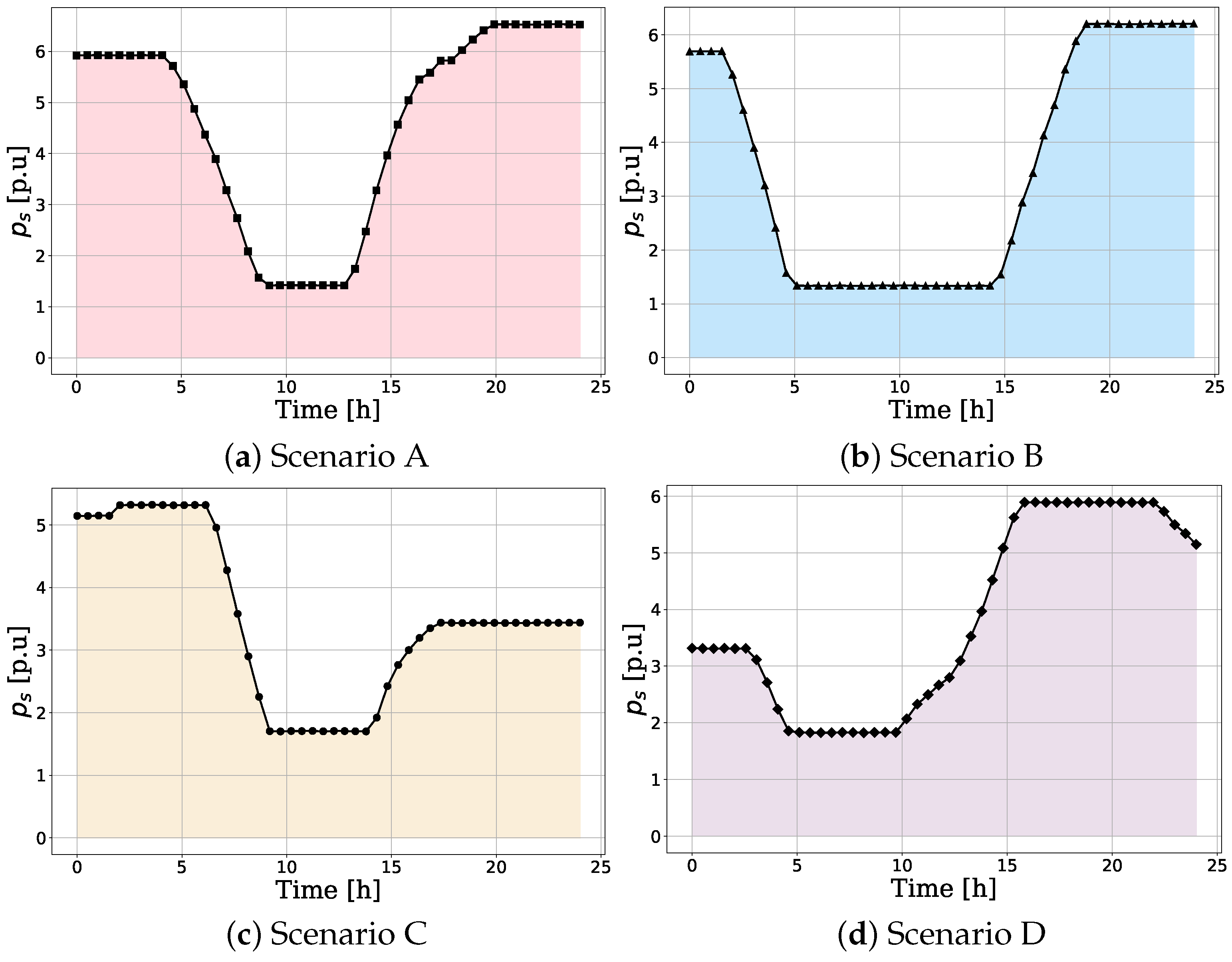
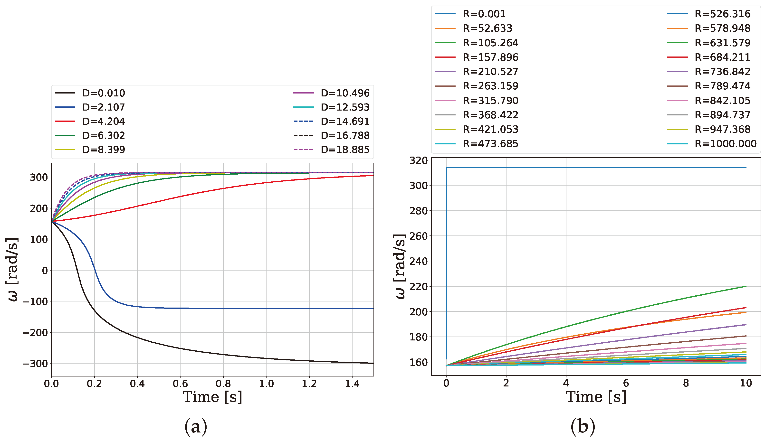
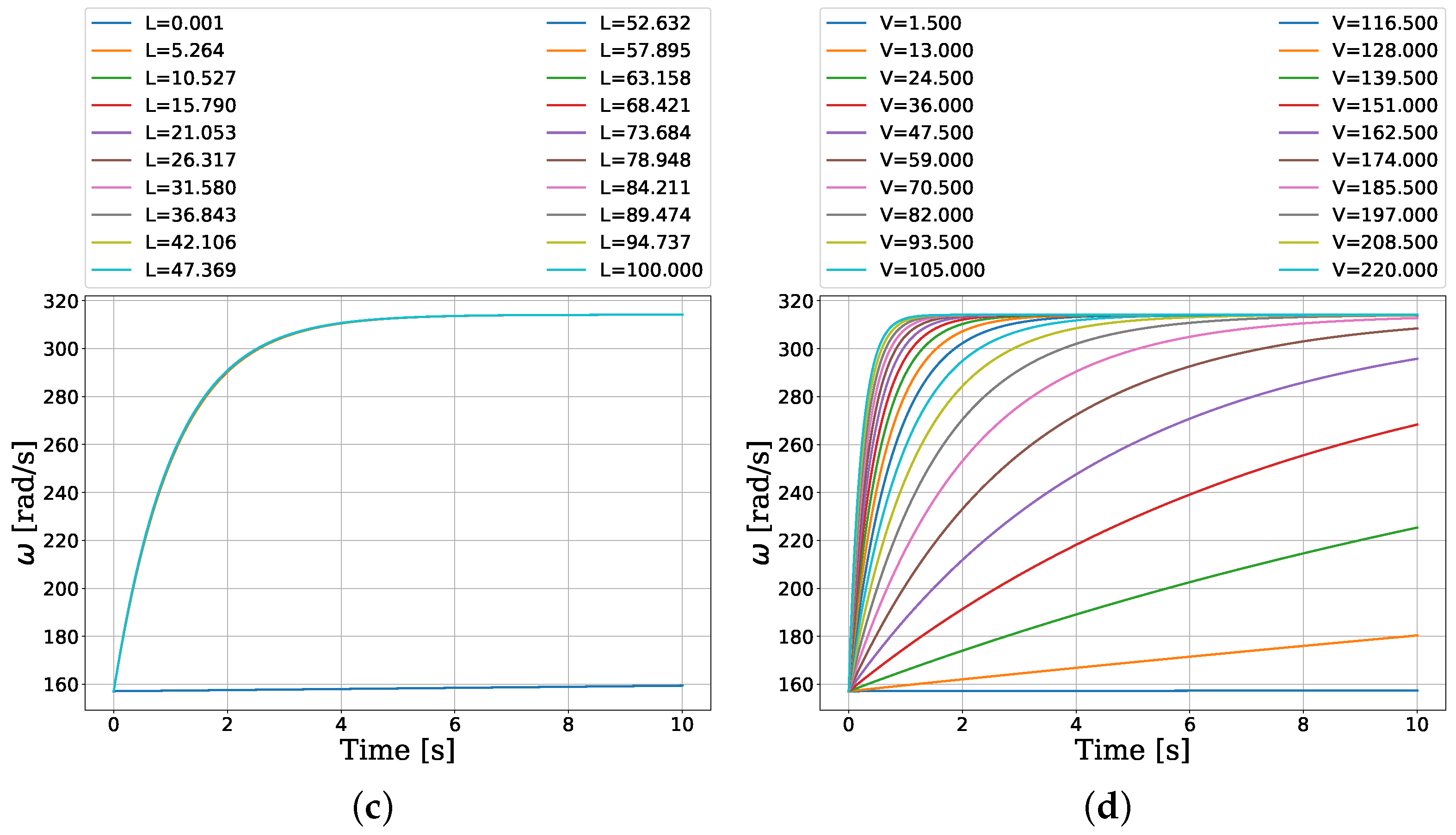
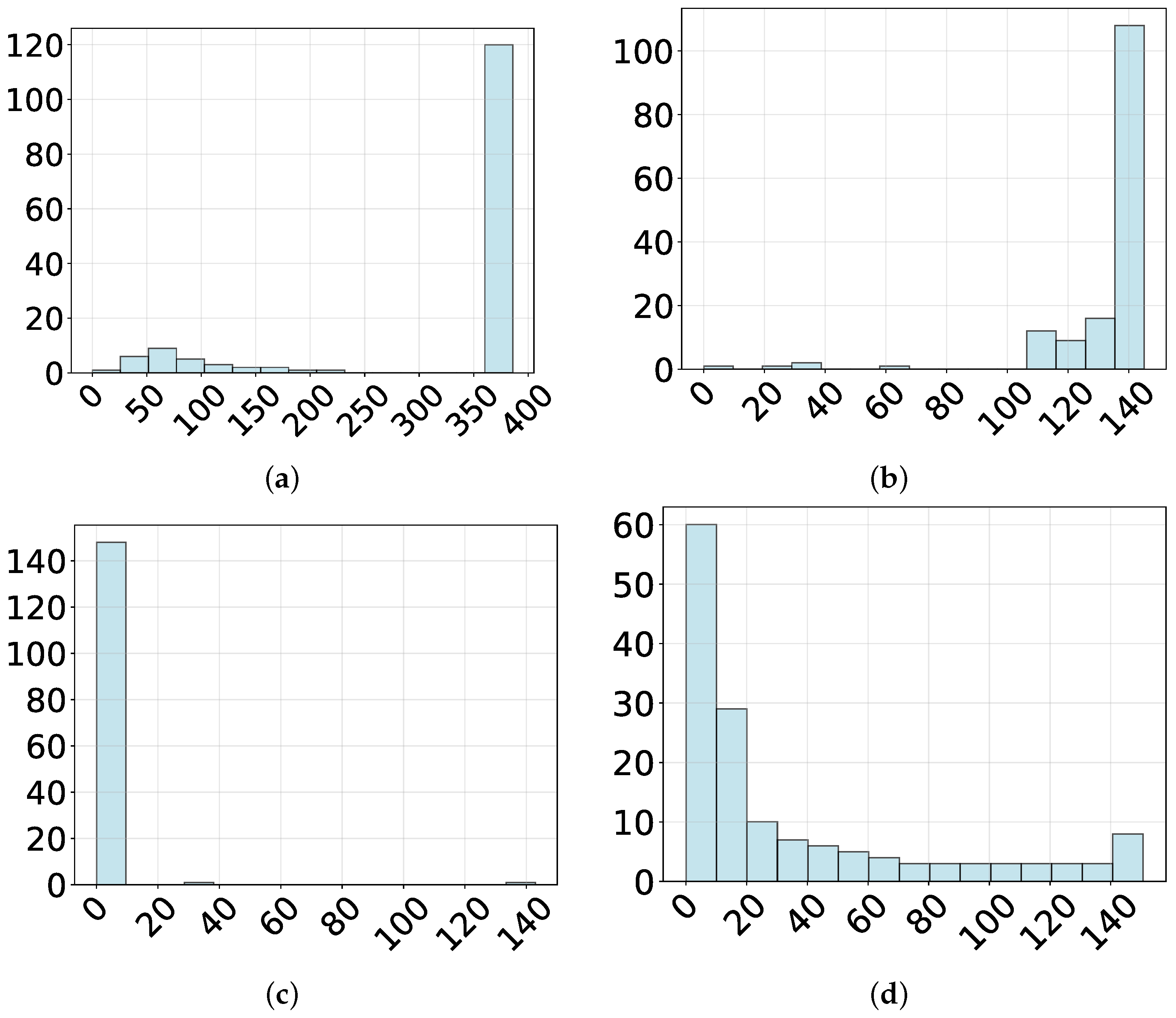
Examine the following non-linear load function:
P load ( ω ) = τ ( ω ) · ω ,
where τ ( ω ) is given by
α · ω , ω ω 0 α · ω 0 , ω > ω 0 ,
where α = P ref ω s 2 .
To prove that ω = ω s is indeed the global asymptotic stable point, we aim to prove that the conditions of Theorem 1 hold. We start by analyzing separately the domains [ 0 , ω 0 ] and ( ω 0 , ) . Define two constants for each domain c l 0 ,   c u > 0 which denote the upper and lower bound of τ ( ω ) accordingly. Following this, the global upper and lower bounds are given by k = max { c u 1 , c u 2 } and D = min { c l 1 , c l 2 } , where the superscript i { 1 , 2 } denotes the domain. Consider the domain [ 0 , ω 0 ] ; the expression that we are interested in is given by
P load ( ω ) P ref ω ω s .
Alternatively, we have
P ref ω s 2 · ω 2 P ref ω ω s ,
which is equal to
P ref ω s · ( ω ω s ) 2 1 ω ω s 1 .
This can be further simplified as follows:
P ref ω s · ω ω s + 1 .
Using the extreme value theorem, since the expression (50) is continuous on a closed and bounded interval [ 0 , ω 0 ] , it must attain a minimum and maximum value there. Moreover, since the function is monotonic, it is assured that it will attain them only once on this interval. Hence, (53) is bounded from below by c l 1 = 0 , and since it is monotonically increasing, the maximum value is obtained at ω 0 and equals to c u 1 = P ref ω s · ( ω 0 ω s + 1 ) . Next, looking at the domain ( ω 0 , ) , substituting (48) in Expression (50) equals
P ref ω s 2 · ω 0 · ω P ref ω ω s ,
which yields
P ref ω s · ω 0 ω s · ω ω s 1 ω ω s 1 .
Note that ω 0 ω s > 1 since ω 0 > ω s . Hence, the function (55) is continuous and strictly monotonically decreasing on the interval ( ω 0 , ) , which leads to a lower bound as follows:
c l 2 = P ref ω s · ( ω 0 ω s ) 2 1 ω 0 ω s 1 ,
which reduces to
c l 2 = P ref ω s · ω 0 ω s + 1 .
The upper bound on this interval can be calculated by examining the limit ω , which is
lim ω P ref ω s · ω 0 ω s · ω ω s 1 ω ω s 1 = P ref ω s · ω 0 ω s .
Consequently, we can choose c u 2 = P ref ω s · ω 0 ω s as the upper bound on the current interval. Summarizing, we can globally bound (50) from below by
D = max 0 , P ref ω s · ω 0 ω s + 1 = P ref ω s · ω 0 ω s + 1 ,
where the global upper bound is
k 0 = max P ref ω s · ( ω 0 ω s + 1 ) , P ref ω s · ω 0 ω s = P ref ω s · ω 0 ω s + 1 .
This proves that the conditions of Theorem 1 hold, and therefore ω = ω s is indeed the global asymptotic equilibrium point, as desired.

3. Numeric Results

To demonstrate this result, we consider here the classical problem of managing an ideal grid-connected storage device, and focus on the behavior of the poles given different values of the damping coefficient of the generator. Consider a microgrid system comprising a grid-connected ideal storage device and a photovoltaic (PV) panel, as illustrated in Figure 4.
The storage device is charged by both the grid and the PV, and supplies an aggregated load characterized by its active power consumption. The load’s active power demand, represented by a continuous, positive function P a : R 0 R , is defined over a finite time interval [ 0 , T ] , where T is a known constant. The power generated by the PV panel is modeled as a piecewise continuous, non-negative function P p v : R 0 R . The net power consumption of the load is given by P L ( t ) = P a ( t ) P p v ( t ) . The rate of charge or discharge of the storage device is described by P s ( t ) = P g ( t ) P L ( t ) , where P g : R 0 R is the power supplied by the grid, and P s : R 0 R is the power flowing into the storage device. Additionally, the quantities E g ( t ) ,   E L ( t ) , and E s ( t ) represent the generated energy, the load energy, and the stored energy, respectively. These energy values are derived from their corresponding power functions via the relation E ( t ) = 0 T P ( τ ) d τ .
To verify our findings, we performed a MATLAB simulation, using Simulink to model the storage device as an R-L circuit, using the idea presented in [30] and the analysis presented in Section 2.3. The solar generation and the consumption profiles are presented in Figure 5.
The critical value of the bound D, which defines the stability condition, is D t h = 95.402 . Performing the simulation for different values of D shows clearly that for all values of D that are above the threshold value D t h , the system is stable and the frequency converges to the globally asymptotically stable point ω s 314 . On the contrary, for all values of D that are beneath the threshold D t h , the system diverges. For values of D in which the system is stable, the scheduling policy of the storage device is presented in Figure 6.
We examine how different values of the damping coefficient, the resistance, the inductance, and the voltage affect the frequency. From Figure 7, it may be observed that the frequency stabilizes on the unique global stable point ω s , or diverges for specific parameters. Specifically, we show how the inherent variability of the non-linear load causes deviation of the frequency trajectory. This is especially interesting since it helps us quantify the notion of resilience analytically, by calculating how the equilibrium point changes in real-world scenarios under changing environmental conditions. Hence, we look at the stable trajectory, denoted by t r s , which divides the plane into two halves: one contains stable trajectories, and the other contains unstable ones. We calculate the Mean Square Error (MSE) between t r s and the rest of the trajectories. Figure 8 presents the results for changing values of the damping coefficient, resistance, inductance, and voltage. We continue the analysis by looking at the root-locus plot of several cases that are presented in Figure 9. First, we examine 100 evenly spaced values of the resistance in the following range R [ 0.1 , 100 ] in units of Ω , and 100 different values of the damping coefficient where D [ 0.01 , D t h + 10 ] . Extending this idea, we examine the pole movement as the values of the damping coefficient D, and the inductance L, or the voltage V change, as may be viewed in the same figure. The same values of the damping coefficient are tested, together with 100 evenly distributed values of the inductance from the range L [ 0.001 , 100 ] in units of Henry, and the same applies to the values of the voltage taken from the range V [ 1.5 , 220 ] , in units of Volts. Finally, it is well known that the amount of production from renewable sources in the system affects the stability of the frequency [6,31,32]. We examined a typical deviation up to 1 Hz from the nominal frequency, and assess how these fluctuations, together with changing load, influence the locations of the poles, and hence the stability of the system.

4. Discussion and Future Work

The Popov stability criterion allows a systematic exploration of global stability properties of nonlinear dynamic systems that contain a single memory-less nonlinear element, and a general linear subsystem. To emphasize the strengths of this criterion, we briefly compare it to other tools for stability analysis. Naturally, this topic is extremely broad, and only a few highlights are given in the current discussion. The Popov stability criterion may be derived directly using a suitable Lyaponuv function; hence, it represents a private case of this more general method. The existence of a Lyapunov function is a necessary and sufficient condition for the stability of an equilibrium point. In some specific cases, the construction of Lyapunov functions is possible using a predefined method. A well-known example is the Lyapunov function of a linear system, V ( x ) = x T P x , where P is the solution of the Lyapunov equation A T P + P A + Q = 0 , in which A is the state matrix, and Q is any positive definite matrix. Yet, there is no general technique for constructing Lyapunov functions for general nonlinear systems. In this sense, the Popov criterion allows a simple and structured method for assessing the stability of a system with (a single) non-linearity, and allows for determining the global stability of an equilibrium point.
Another well-known approach for stability analysis is the linearization of a nonlinear system in the neighborhood of an equilibrium point. This approach is very general, and can be implemented in many types of systems; however, its main disadvantage is that the results are only local—that is, this approach provides no information regarding the Region-of-Attraction (RoA) of an equilibrium point, and says nothing about its global asymptotic stability. We also obtain no information regarding other equilibrium points of the dynamic model. In this light, we once again emphasize the main advantage of the Popov criterion, which enables determining the global asymptotic stability of an equilibrium point in a methodical and straight-forward manner, providing a more comprehensive understanding of the system’s behavior. However, the main drawback of Popov’s criterion is that it only applies to systems with a single non-linearity, or a non-linearity that occurs in one dimension. To overcome this challenge, in large systems, or systems with multiple non-linearities, we may aggregate different components, and analyze them step-by-step.
Regarding future work, the present work focuses on applications of Popov’s stability criterion for exploring frequency stability in various small-scale power systems models. While this criterion is a useful tool for analyzing small-scale systems, several directions for future research remain open. One possible line of work investigates the application of this principle to components used as ancillary services that appear in smart grids. For instance, consider Synchronverters [33], which act similarly to synchronous generators to provide inertia to the grid. The nonlinear dynamics of these units make stability analysis critical, particularly in scenarios involving the high penetration of distributed energy resources. The systematic application of the Popov criterion to Synchronverter models could provide deeper insights into their global stability properties, and may allow exploration of their design and operation in modern smart grids. Another area of exploration is adapting the proposed method to analyze systems with multiple non-linearities. Many modern power systems, particularly those incorporating a high amount of renewable energy, exhibit complex dynamics resulting from the interaction of various non-linear components. Extending the current stability criterion to account for multiple interacting non-linearities would enhance its applicability to large-scale systems and allow for a more comprehensive understanding of frequency behaviors in distributed energy systems. Additionally, the analytical conditions derived from the Popov criterion could lay the foundation for designing real-time controllers that ensure stable operation under dynamic conditions. These controllers may be particularly useful in several scenarios, especially in areas with high generation from renewable sources, and for emergency control. Future work can also focus on developing algorithms and control strategies that use the concepts of the proposed global stability analysis to monitor and maintain system stability in real time.

5. Conclusions

Stability problems in power systems are typically explored using one of three main approaches: numerical methods, linearization techniques, or direct methods, which utilize Lyapunov energy functions. This paper belongs to the third category, and highlights the usefulness of the Popov stability criterion in the analysis of nonlinear power system models. The main advantage of this criterion is that it provides conditions for global asymptotic stability of an equilibrium point. This stands in contrast to linearization techniques, which only provides conditions for local stability. We showed a general method for applying this stability criterion, and examined its uses in several specific applications. More specifically, we examined small power systems such as synchronous machines driving a resistive-inductive load and a synchronous machine driving a lossless synchronous motor with a quasi-linear mechanical load. Following this, we relied on a simplified model of a storage device that is powered by a synchronous machine to analyze the frequency stability for varying system parameters. For instance, we evaluated for which practical parameters of the storage and the synchronous machine, such as the resistance and damping coefficient, the equilibrium was globally asymptotically stable.

Author Contributions

Conceptualization, E.G.-G. and Y.L.; methodology, Y.L.; software, E.G.-G. and Y.L.; validation, E.G.-G., J.B. and L.K.; formal analysis, E.G.-G. and Y.L.; writing—original draft preparation, E.G.-G.; writing—review and editing, E.G.-G. and Y.L.; visualization, E.G.-G. and J.B.; supervision, Y.L.; Funding acquisition J.B. All authors have read and agreed to the published version of the manuscript.

Funding

The work of J. Belikov was partly supported by the Estonian Research Council grant PRG1463.

Data Availability Statement

The original data presented in the study are openly available on GitHub at https://data.nrel.gov/submissions/156, available on 30 November 2024.

Conflicts of Interest

Author Liran Katzir was employed by the company Advanced Energy Industries. The remaining authors declare that the research was conducted in the absence of any commercial or financial relationships that could be construed as a potential conflict of interest.

References

  1. Kundur, P. Power System Stability and Control; McGraw-Hill: New York, NY, USA, 1994. [Google Scholar]
  2. Kundur, P.; Paserba, J.; Ajjarapu, V.; Andersson, G.; Bose, A.; Canizares, C.; Hatziargyriou, N.; Hill, D.; Stankovic, A.; Taylor, C.; et al. Definition and classification of power system stability IEEE/CIGRE joint task force on stability terms and definitions. IEEE Trans. Power Syst. 2004, 19, 1387–1401. [Google Scholar] [CrossRef]
  3. Caliskan, S.Y.; Tabuada, P. Compositional Transient Stability Analysis of Multimachine Power Networks. IEEE Trans. Control Netw. Syst. 2014, 1, 4–14. [Google Scholar] [CrossRef]
  4. Fernández-Guillamón, A.; Gómez-Lázaro, E.; Muljadi, E.; Molina-García, Á. Power systems with high renewable energy sources: A review of inertia and frequency control strategies over time. Renew. Sustain. Energy Rev. 2019, 115, 109369. [Google Scholar] [CrossRef]
  5. Meegahapola, L.; Sguarezi, A.; Bryant, J.S.; Gu, M.; Conde D, E.R.; Cunha, R.B.A. Power System Stability with Power-Electronic Converter Interfaced Renewable Power Generation: Present Issues and Future Trends. Energies 2020, 13, 3441. [Google Scholar] [CrossRef]
  6. Bevrani, H.; Ghosh, A.; Ledwich, G. Renewable energy sources and frequency regulation: Survey and new perspectives. IET Renew. Power Gener. 2010, 4, 438–457. [Google Scholar] [CrossRef]
  7. Golpîra, H.; Atarodi, A.; Amini, S.; Messina, A.R.; Francois, B.; Bevrani, H. Optimal Energy Storage System-Based Virtual Inertia Placement: A Frequency Stability Point of View. IEEE Trans. Power Syst. 2020, 35, 4824–4835. [Google Scholar] [CrossRef]
  8. Mosca, C.; Arrigo, F.; Mazza, A.; Bompard, E.; Carpaneto, E.; Chicco, G.; Cuccia, P. Mitigation of frequency stability issues in low inertia power systems using synchronous compensators and battery energy storage systems. IET Gener. Transm. Distrib. 2019, 13, 3951–3959. [Google Scholar] [CrossRef]
  9. Serban, I.; Teodorescu, R.; Marinescu, C. Energy storage systems impact on the short-term frequency stability of distributed autonomous microgrids, an analysis using aggregate models. IET Renew. Power Gener. 2013, 7, 531–539. [Google Scholar] [CrossRef]
  10. Süli, E.; Mayers, D.F. An Introduction to Numerical Analysis; Cambridge University Press: Cambridge, UK, 2003. [Google Scholar]
  11. Nielsen, K.L. Methods in Numerical Analysis.; MACMILLAN: New York, NY, USA, 1956. [Google Scholar]
  12. Montoya, O.D.; Gil-González, W. On the numerical analysis based on successive approximations for power flow problems in AC distribution systems. Electr. Power Syst. Res. 2020, 187, 106454. [Google Scholar] [CrossRef]
  13. Socha, L. Linearization Methods for Stochastic Dynamic Systems; Springer Science & Business Media: Berlin/Heidelberg, Germany, 2007. [Google Scholar]
  14. Liang, X. Linearization Approach for Modeling Power Electronics Devices in Power Systems. IEEE J. Emerg. Sel. Top. Power Electron. 2014, 2, 1003–1012. [Google Scholar] [CrossRef]
  15. Sun, J. Small-Signal Methods for AC Distributed Power Systems—A Review. IEEE Trans. Power Electron. 2009, 24, 2545–2554. [Google Scholar] [CrossRef]
  16. Persson, J.; Söder, L. Comparison of threes linearization methods. In Proceedings of the 16th Power System Computation Conference, Power Systems Computation Conference (PSCC), Glasgow, UK, 14–18 July 2008. [Google Scholar]
  17. Slotine, J.J.E. Applied Nonlinear Control; Pearson: London, UK, 1991. [Google Scholar]
  18. Isidori, A. Nonlinear Control Systems: An Introduction; Springer: Berlin/Heidelberg, Germany, 1985. [Google Scholar]
  19. Willems, J. Direct method for transient stability studies in power system analysis. IEEE Trans. Autom. Control 1971, 16, 332–341. [Google Scholar] [CrossRef]
  20. Chang, H.D.; Chu, C.C.; Cauley, G. Direct stability analysis of electric power systems using energy functions: Theory, applications, and perspective. Proc. IEEE 1995, 83, 1497–1529. [Google Scholar] [CrossRef]
  21. Zhai, C.; Nguyen, H.D. Estimating the Region of Attraction for Power Systems Using Gaussian Process and Converse Lyapunov Function. IEEE Trans. Control Syst. Technol. 2022, 30, 1328–1335. [Google Scholar] [CrossRef]
  22. Kazemi, A.; Motlagh, M.J.; Naghshbandy, A. Application of a new multi-variable feedback linearization method for improvement of power systems transient stability. Int. J. Electr. Power Energy Syst. 2007, 29, 322–328. [Google Scholar] [CrossRef]
  23. Tzounas, G.; Dassios, I.; Milano, F. Small-signal stability analysis of implicit integration methods for power systems with delays. Electr. Power Syst. Res. 2022, 211, 108266. [Google Scholar] [CrossRef]
  24. Kannan, A.; Nuschke, M.; Dobrin, B.P.; Strauß-Mincu, D. Frequency stability analysis for inverter dominated grids during system split. Electr. Power Syst. Res. 2020, 188, 106550. [Google Scholar] [CrossRef]
  25. Soultanis, N.L.; Papathanasiou, S.A.; Hatziargyriou, N.D. A Stability Algorithm for the Dynamic Analysis of Inverter Dominated Unbalanced LV Microgrids. IEEE Trans. Power Syst. 2007, 22, 294–304. [Google Scholar] [CrossRef]
  26. Gu, Y.; Green, T.C. Power System Stability with a High Penetration of Inverter-Based Resources. Proc. IEEE 2023, 111, 832–853. [Google Scholar] [CrossRef]
  27. Arul, P.; Ramachandaramurthy, V.K.; Rajkumar, R. Control strategies for a hybrid renewable energy system: A review. Renew. Sustain. Energy Rev. 2015, 42, 597–608. [Google Scholar] [CrossRef]
  28. Nassar, I.; Elsayed, I.; Abdella, M. Optimization and Stability Analysis of Offshore Hybrid Renewable Energy Systems. In Proceedings of the 2019 21st International Middle East Power Systems Conference (MEPCON), Cairo, Egypt, 17–19 December 2019; pp. 583–588. [Google Scholar] [CrossRef]
  29. Aggarwal, J.K.; Johnson, S. Notes on Nonlinear Systems. 1977. Available online: https://www.amazon.com/Nonlinear-Systems-Jagdishkumar-Keshoram-Aggarwal/dp/0442202636 (accessed on 19 December 2024).
  30. Yang, J.; Cai, Y.; Pan, C.; Mi, C. A novel resistor-inductor network-based equivalent circuit model of lithium-ion batteries under constant-voltage charging condition. Appl. Energy 2019, 254, 113726. [Google Scholar] [CrossRef]
  31. Shobayo, L.O.; Dao, C.D. Smart Integration of Renewable Energy Sources Employing Setpoint Frequency Control—An Analysis on the Grid Cost of Balancing. Sustainability 2024, 16, 9906. [Google Scholar] [CrossRef]
  32. Dreidy, M.; Mokhlis, H.; Mekhilef, S. Inertia response and frequency control techniques for renewable energy sources: A review. Renew. Sustain. Energy Rev. 2017, 69, 144–155. [Google Scholar] [CrossRef]
  33. Zhong, Q.C.; Weiss, G. Synchronverters: Inverters That Mimic Synchronous Generators. IEEE Trans. Ind. Electron. 2011, 58, 1259–1267. [Google Scholar] [CrossRef]
Figure 1. Block diagram of the system based on [29].
Esa 01 00005 g001
Figure 2. Geometrical representation of the Popov stability criterion, based on [29].
Esa 01 00005 g002
Figure 3. Standard first-order synchronous generator model, which is based on time-varying phasors.
Esa 01 00005 g003
Figure 4. System model consisting of three buses, bumered 1–3. A generator is connected to bus number 1, a PV is connected to bus number 2, feeding a non-linear load that includes a storage device, both connected to bus number 3.
Esa 01 00005 g004
Figure 5. Solar generation and consumption profiles for various scenarios.
Esa 01 00005 g005
Figure 6. Storage scheduling policies under different scenarios of solar generation and consumption profiles.
Esa 01 00005 g006
Figure 7. The influence of different system parameters on the frequency. (a) Frequency behavior for changing values of D. (b) Frequency behavior for changing values of R. (c) Frequency behavior for changing values of L. (d) Frequency behavior for changing values of V.
Esa 01 00005 g007aEsa 01 00005 g007b
Figure 8. MSE calculations for changing parameters. (a) MSE for changing values of D; (b) MSE for changing values of R; (c) MSE for changing values of L; (d) MSE for changing values of V.
Esa 01 00005 g008
Figure 9. Root-locus for changing parameters. (a) Root-locus for changing values of damping coefficient and resistance. (b) Root-locus for changing values of damping coefficient and voltage. (c) Root-locus for changing values of damping coefficient and inductance. (d) Root-locus for changing values of resistive load and frequency fluctuations.
Esa 01 00005 g009
Disclaimer/Publisher’s Note: The statements, opinions and data contained in all publications are solely those of the individual author(s) and contributor(s) and not of MDPI and/or the editor(s). MDPI and/or the editor(s) disclaim responsibility for any injury to people or property resulting from any ideas, methods, instructions or products referred to in the content.

