Article

Model-Assisted Probabilistic Neural Networks for Effective Turbofan Fault Diagnosis

by
Christoforos Romesis
*,
Nikolaos Aretakis
and
Konstantinos Mathioudakis
Laboratory of Thermal Turbomachines, School of Mechanical Engineering, National Technical University of Athens, 15710 Athens, Greece
*
Author to whom correspondence should be addressed.
Aerospace 2024, 11(11), 913; https://doi.org/10.3390/aerospace11110913
Submission received: 23 September 2024 / Revised: 31 October 2024 / Accepted: 4 November 2024 / Published: 6 November 2024
(This article belongs to the Special Issue Machine Learning for Aeronautics (2nd Edition))

Abstract

:
A diagnostic method for gas-path faults of turbofan engines, relying on a Probabilistic Neural Network (PNN) coupled with a thermodynamic model of the engine, is presented. The novel aspect of the method is that its training information is generated dynamically by an accompanying Engine Performance Model. In the proposed approach, the PNN efficiently addresses the first step of a diagnostic process (i.e., detection of the faulty component at the current operating point), while with the aid of an adaptive engine model, the fault is then further isolated and identified. A description of the proposed method and training aspects of the PNN are presented. The method is applied to the case of a mixed-flow turbofan engine to diagnose common gas-path faults in compressors and turbines (i.e., fouling, FOD, erosion, and tip clearance). Its performance is evaluated using realistic fault data that may be acquired at various operating conditions within a flight envelope.

1. Introduction

Numerous methods allowing the diagnosis of gas turbine engine faults have been proposed by researchers over the years. Concise and in-depth reviews of existing diagnostic methods are provided in [1,2,3], while reviews in [4,5] also cover the part of prognostics. These reviews describe the most existing diagnostic methods, including discussions of their advantages, disadvantages, and application fields. Reviews of diagnostic methods that rely on tools that have emerged in recent years, namely artificial intelligence techniques, are provided in [6,7,8,9]. Zhou and Huang [10] review modeling, control, and diagnostic methods, focusing more on challenges and prospects for future research. A common feature of diagnostic methods is that they rely on the basic principle that a fault results in deviations of engine parameters that represent the engine’s health condition. Mathioudakis et al. [11] provide a review of the most common faults in gas turbine compressors and turbines (fouling, Foreign-Object-Damage (FOD), tip clearance, and erosion). Their review showed a specific association between these physical faults and parameters representing engine component health. Similar associations have been reported in [3,4,5].
Diagnostic methods for gas-path faults fall into two main categories: (a) model-based methods and (b) data-driven methods.
In model-based methods, the core tool for diagnostic reasoning is based on engine thermodynamic models, where the relationship among the parameters involved is determined through explicit mathematical and thermodynamic equations. Such model-based methods represent physical faults through component performance parameter deviations and estimate these parameters from acquired measurements. Various model-based gas-path diagnostic methods have been developed since Gas-Path Analysis (GPA) was first introduced by Urban [12] around 1967. Typical examples of such model-based diagnostic methods involve methods based on classical mathematical approaches [13], classical GPA [14], adaptive simulation [15], adaptive GPA [16], performance model zooming at the stage level [17], and the integration of various relevant methods [18]. However, the required information for efficient application is usually not fully available, mainly because of the limited instrumentation set.
Data-driven methods rely on available data acquired from the engine. The data can come from historical records, measurement records from operating engines, or even simulated data generated by an Engine Performance Model. Data-driven methods vary from methods using classical statistical approaches, such as statistical pattern recognition [19], Hidden Markov Models (HMMs) [20], Principal Component Analysis (PCA) [21], and logistic regression [22], to the more complex approaches from deep learning, like Autoencoders [23], Deep Belief Networks (DBNs) [24], Convolutional Neural Networks (CNNs) [25,26], and Recurrent Neural Networks (RNNs) [26,27].
A conclusion drawn from these works is that deep learning approaches can reveal the interrelations between the observations and states of complex systems, such as engine faults in gas turbine diagnostics, even when only sparse and unlabeled data are available. However, their ability comes at the cost of complexity. Building and maintaining a deep learning model requires close collaboration between AI and domain experts, while high computational resources and time are generally required to train and apply such models. Thus, it is not surprising that many classical machine learning approaches are, in many cases, preferred by many researchers. Such approaches may provide a suitable diagnostic solution in the following cases:
-
The diagnostic problem can be simplified/narrowed (for example, in cases where only fault detection is required);
-
A large amount of relevant data are available (for example, in cases where a performance model is available);
-
Simplicity is a factor.
Non-deterministic machine learning approaches exhibiting such features, which are used for gas turbine diagnostics, include Support Vector Machines (SVMs) [28], Fuzzy Logic [29], kNN [30], Bayesian Belief Networks [31], and Probabilistic Neural Networks (PNNs).
A PNN is a three-layer, feed-forward neural network allowing probabilistic classification [32]. This type of network was introduced by Specht [33], and a recent overview of theory, implementation, and applications can be found in [34]. A PNN estimates the probability that an input pattern is classified into one of several predefined exhaustive and mutually exclusive classes. A PNN for gas turbine diagnosis was first employed by Eustace and Merrington [35] using fleet data. Later, PNN methods, coupled with an EPM, were extensively used to diagnose sensor faults [36], gas-path faults from simulated data of an aircraft engine [37], faults from flight data [38], and gas-path faults of stationary engines [39]. Buttler et al. [40] compared several machine learning methods, including a PNN-based method, for diagnosing turbofan faults. More recent applications of PNNs for gas turbine fault diagnosis [41,42,43] confirm the strong classification ability of this type of neural network.
The present paper proposes a diagnostic method for gas-path fault diagnosis in engine components, using a PNN coupled with an Engine Performance Model (EPM), well adapted to the specific engine [38], and an aerothermodynamic diagnostic tool to derive precise fault features. The primary advantage of PNNs is that ‘training is easy and instantaneous’, to borrow Specht’s words [33]. The training procedure consists of acquiring and feeding to the network a set of training patterns that adequately represent the considered classes, with no need for recursive estimation of network parameters, as is the case for other types of neural networks. However, its efficiency depends on how well the operating conditions and fault situations are represented. A large amount of information may be needed to cover the envelope of operating conditions sufficiently. Since this coverage is essentially at discrete operating points, when operating conditions not covered in the training set are encountered, the PNN becomes less efficient. The method proposed here tackles these limitations. The training set is generated dynamically. Instead of storing many patterns corresponding to the combination of many operating conditions, faults, and fault features, patterns are generated with the aid of an engine model precisely at the conditions at which test data are collected.
The remainder of this paper is organized as follows. Section 2 describes the Engine Performance Model and how some of the most common physical faults can be expressed in terms of the parameters involved in the EPM. Section 3 describes the proposed diagnostic method, beginning with an overview of the proposed method and then providing a detailed description of its constituent parts. Section 4 presents the application of the method to a mixed-flow turbofan. First, the engine and specifics for applying the diagnostic method to that engine are described. The training and testing patterns are then presented, followed by the diagnostic results.

2. Engine Performance Model and Representation of Physical Faults

An Engine Performance Model (EPM) interrelates parameters that represent engine component health and operating conditions with measurements performed on an engine [44] and can be expressed through the following equation [15]:
Y = g ( u , f )
where g is a vector function representing the EPM, u is a vector of measured quantities that define the engine operating point, Y is a vector consisting of a set of measurements used for condition monitoring, and f is the vector of engine component ‘health parameters’. Two such ‘health parameters’ are most commonly used for each engine component. For a component with entrance at station ‘c’ along the engine, these parameters are
Flow   factor :   SW c = W c · T c / p c / W c · T c / p c ref
Efficiency   factor :   S E c = n c / n c r e f
where W c is the gas mass flow rate, T c is the total temperature, p c is the total pressure at station ‘c’, and n c is the component efficiency. The subscript ‘ref’ indicates reference values, i.e., values for a healthy engine.
The use of such parameters to describe the health condition of engine components was discussed in [15]. The deviation of an engine component health parameter from its nominal value indicates the presence of a fault in the corresponding component. Moreover, the more severe the fault, the greater the deviation. The deviation (‘Delta’) of a health parameter fc is defined as follows:
Δ f c % = f c f o c f o c · 100 %
In this equation, f c is the health parameter value, and f o c is its nominal value.
Through an EPM, the nominal values of the measured quantities used for condition monitoring Y o , at a given operating point u , can be calculated. These values correspond to the nominal values of health parameters f o and are thus calculated as follows:
Y o = g u , f o
Once a measurement vector Y is acquired from an engine, the percentage deviation (‘Delta’) of a measurement Y x from its nominal value Y o x is defined as
Δ Y x % = Y x Y o x Y o x · 100 %
When deviations are of small magnitude, the relationship (5) can be linearized to produce a simple relation between measurement and health parameter deviations:
Δ Y = J · Δ f
where J is the Jacobian matrix of function g given by Equation (5), which associates the vector of measurement deviations Δ Y with that of health parameters Δ f .
This relation can generate vectors Δ Y when the deviations Δ f for a fault are known. It has been discussed extensively in [11] that the ratio of the two health component deviations can be used as a characteristic parameter for different faults, such as fouling, tip clearance, erosion, and FOD. The faulty conditions correspond to points on a diagnostic plane that lie along a straight line, different for different faults. Figure 1 illustrates the ratios representing the fouling, tip clearance, erosion, and FOD of gas turbine compressors and tip clearance and erosion of turbines. Two cross-plots of mass flow factor deviation (Δ SW c ) versus deviation of efficiency factor (Δ S E c ) for compressors and turbines, respectively, are shown. Each fault is represented by a line on the plots, corresponding to one fault ratio for each fault. This representation forms the basis of the proposed diagnostic method described in the following section.

3. Method Description

The proposed method is a two-step approach: first, the component suffering from a fault is detected, and then the fault is identified. A flow chart of the method is presented in Figure 2. A PNN allows engine health assessment from aero-thermodynamic measurements acquired from the engine. It uses information from an EPM, with a knowledge base of engine faults. The PNN provides the engine health assessment to predict the most probable engine health condition among a predefined set of possible health conditions. This set comprises health conditions that represent the healthy operation of the engine and the case in which a fault occurs at any of the rotating components of the engine. When a fault is detected, the measurement data are further processed through an aerothermal diagnostic procedure to determine the specific characteristics of the fault.
The diagnostic method’s input information is a vector of measurements acquired from the engine. These measurements are preprocessed with the aid of the EPM, producing deltas of measurements Δ Y and the Jacobian matrix J at the current operating point.
The measurement deltas Δ Y are fed to the PNN. The network’s output is the probability of each set of predefined classes. An example of such classes is as follows:
  • One class, representing the healthy operation of the engine;
  • Additional classes, each representing a faulty engine component operation.
This choice was made because it produced the best diagnostic performance compared with other alternatives. An alternative, for example, would be to have more than one class per component, i.e., one class for each component fault covered.
To estimate the probability of each class, the network is equipped with a set of training patterns, noted as tpij. A training pattern is a vector of simulated measurement deltas (vector Δ Y ) from an engine at one of the predefined health conditions. Several training patterns, representing deviations of the corresponding health parameters at various ratios, are needed for each health condition. The conventional approach generates an extensive set of such patterns that cover all possible operating conditions and fault cases. This choice may lead to a large amount of data, while operating conditions that have not been considered may still be encountered, leading to reduced diagnostic efficiency.
The novel aspect of the proposed approach is that these training patterns are not generated a priori. Instead, they are produced each time we acquire a measurement vector and represent the training patterns at the specific engine operating point from which the data come. This is achieved by employing a knowledge base, as illustrated in Figure 2. The knowledge base encompasses engine physical faults, with the deltas of engine health parameters Δ f . The values of the training patterns are calculated from Δ f and the Jacobian matrix J (Equation (7)).
The PNN produces the probabilities for each of the considered engine conditions. The condition with the maximum probability is the one considered to be the current condition of the engine. If the maximum probability represents the healthy operation of the engine, the diagnostic procedure is terminated. If it represents a fault, a step further is taken to estimate the magnitude of deviation of the health parameters of the component found faulty, from which the physical fault is identified. Therefore, the diagnostic method described above consists of four parts, as illustrated in Figure 2.
  • Measurements preprocessing;
  • Engine health assessment;
  • Generation of training patterns;
  • Health assessment post-process.
  • These parts are described in more detail in the following paragraphs.

3.1. Measurements Preprocessing

Given the vectors of measurements u and Y , the EPM produces the following:
-
The nominal values of the measured quantities used for condition monitoring Yo, for the given operating point u . The delta ΔYx of a measurement, Yx, is then calculated as the percentage deviation of the Yi from its nominal value Yox;
-
The Jacobian matrix J , at the specific operating point.

3.2. Engine Health Assessment

At this step, the PNN produces the probability of occurrence of each predefined class, given the input deviation pattern. The PNN is shown in Figure 2. The input layer nodes represent the available measurement deviations Δ Y . One node is considered for each available measurement.
The nodes of the middle layer represent the training patterns. One node represents one training pattern, which is a vector of deltas of simulated measurements Y coming from one of the engine’s considered health conditions. These training patterns are generated at the ‘generation of training patterns’ part of the diagnostic method, as presented in the next paragraph.
The output layer nodes represent the classes to which an examined input pattern (i.e., Δ Y ) can be classified. For the problem at hand, each class represents a different health condition of the engine (as already mentioned, one class is for the healthy operation of the engine, and one class is per rotating engine component, which represents cases of fault located at this component).
The network output is the set of probabilities of the considered classes. Each class (health condition) is assigned a probability, given the input deltas Δ Y , calculated through [31].
P C l a s s i Δ Y = P C l a s s i P Δ Y · 2 π n / 2 · σ n · m i · j = 1 m i e x p | Δ Y t p i j | 2 2 σ 2
In this equation:
P C l a s s i Δ Y is the output probability of the health condition of the engine represented by Class − i of the network, given the input deltas ΔY.
P C l a s s i is the a priori probability of the health condition of the engine represented by Class − i of the network. Each health condition is considered to have an equal a priori probability, thus: P C l a s s i = 1 k , where k is the number of considered classes.
P Δ Y is the a priori probability of the input deltas ΔY. This acts as a normalization factor. As the considered classes are considered exhaustive and mutually exclusive, the sum of probabilities of all classes, given the input deltas ΔY, should be equal to 1. Therefore:
i = 1 k P C l a s s i Δ Y = 1 = >  
i = 1 k P C l a s s i P Δ Y · 2 π n 2 · σ n · m i · j = 1 m i e x p | Δ Y t p i j | 2 2 σ 2 = 1 = >  
P Δ Y · i = 1 k P C l a s s i 2 π n 2 · σ n · m i · j = 1 m i e x p | Δ Y t p i j | 2 2 σ 2 = 1 = >  
P Δ Y = 1 i = 1 k P C l a s s i 2 π n 2 · σ n · m i · j = 1 m i e x p | Δ Y t p i j | 2 2 σ 2
σ is a smoothing factor that is calculated experimentally. A typical initial value is, generally, 0.1 for all classes, which is the value also considered here.
n is the dimension of vector ΔY.
m i is the number of training patterns of Class − i.
Δ Y is the input deltas vector.
t p i j is the j-th training pattern of Class − i.

3.3. Generation of Training Patterns

The PNN training patterns are generated using a knowledge base of the engine conditions, i.e., healthy and faulty with various faults. Each condition is represented through an appropriate pair of Δ f . The way information is stored is based on the representation discussed in Section 2. Patterns of a fault correspond to points lying around a straight line whose slope corresponds to a specific fault, Figure 3. The farther away from the origin, the more severe the fault. Points within the light red sector represent one fault, accounting for some inherent variability or noise in estimating the health factors.
The blue square around the origin indicates cases where none of the health parameters deviate more than a threshold h%, below which no fault is considered to occur at the component. The magnitude of h is case-dependent and relies on the knowledge of the engineer who sets up the diagnostic method for a particular engine.
Point-j at a fault condition, Figure 3, is defined using the values of the following two quantities:
F a u l t M a g n i t u d e j = Δ S W c Δ S W c · Δ S W c 2 + Δ S E c 2 = L c j
F a u l t R a t i o j = Δ S W c / Δ S E c = t a n ( θ c j )
The actual deviations of the health parameters are generated from the values of these quantities. Given a pair ( L c j , tan(θcj)), the corresponding training pattern tpij is generated by computing the corresponding SWc, SEc and then generating the simulated measurement deviations as follows:
Δ S W c = L c j · t a n ( θ c j ) 1 t a n ( θ c j ) 2 + 1
Δ S E c = Δ S E c t a n ( θ c j )
The training pattern is then generated using the Jacobian:
t p i j = Δ Y 1 Δ Y 2 Δ Y n = J · 0 0 Δ S W c Δ S E c 0 0
This procedure is followed for several cases that constitute a sufficient set of training patterns. Later, an application example is provided to elucidate this.

3.4. Fault Identification

The PNN generates probabilities for the input vector based on the training patterns. These probabilities are then assessed to infer which fault occurs, if any, given the vectors of input measurements u and Y. In the proposed method, we consider cases in which only one fault in a single component may be present at a time (the simultaneous presence of more faults is not considered).
We first infer that the existing health condition of the engine is represented by Class-I, which is tied to the highest estimated probability by the PNN among all classes:
P C l a s s i Δ Y = max { P C l a s s j Δ Y , j = 1 , k }
There are two options:
(a)
If the condition with the greatest probability represents healthy operation, the diagnostic procedure ends.
(b)
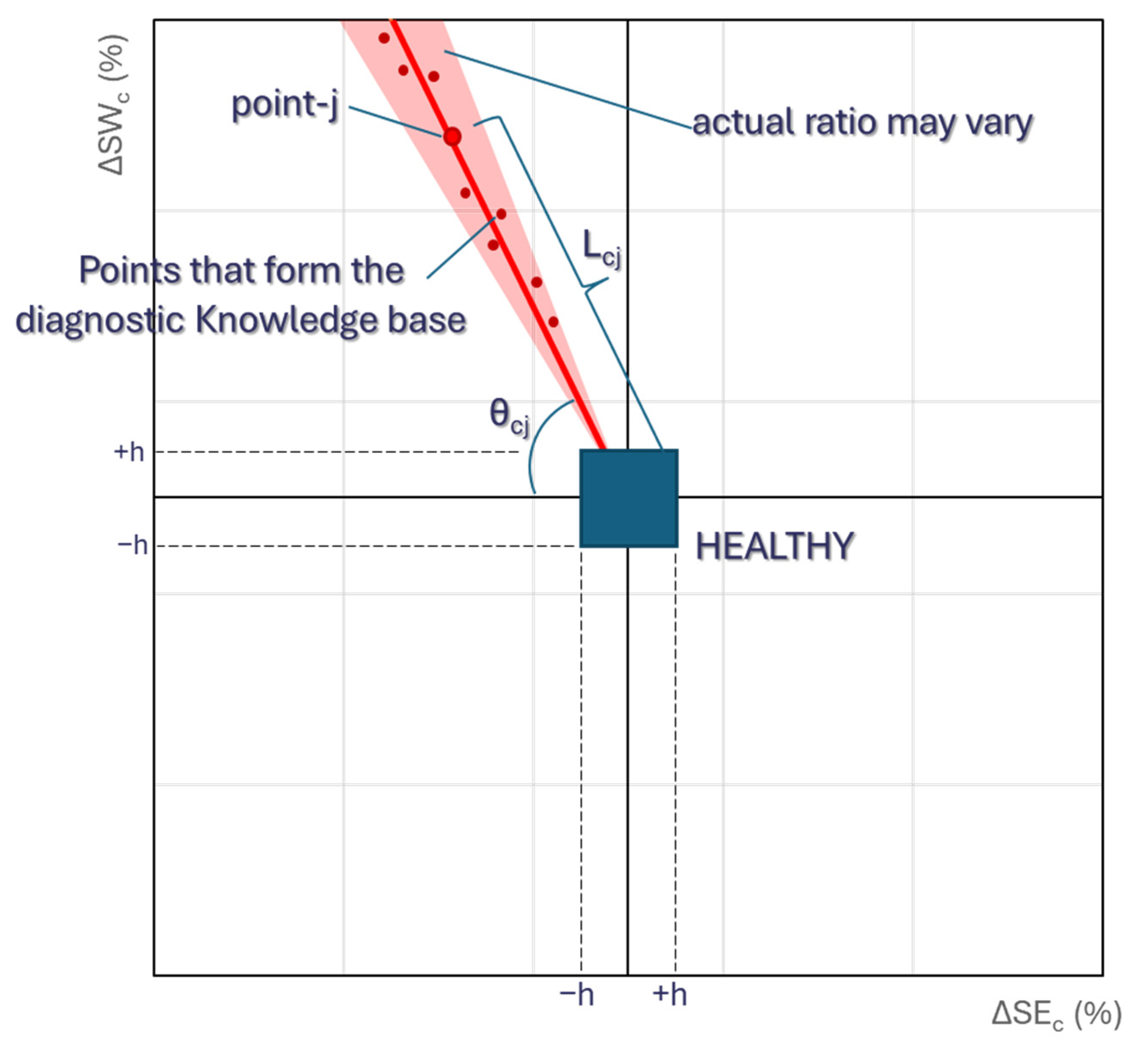
If any other class is tied with the maximum probability, a fault is considered to exist at the corresponding component. If the fault is located at a component with health parameters SWc and SEc, then the following is performed:
  • We estimate the deviation of parameters SWc and SEc through the Jacobian pseudoinverse (PINV) equation as follows:
    Δ f 2 x 1 = J n x 2 1 · Δ Y = J n x 2 T · J n x 2 1 · J n x 2 T · Δ Y
    Δ f 2 x 1 is the vector of deviations of the health parameters:
    Δ f 2 x 1 = Δ S W c Δ S E c
    ΔY is the vector of deltas of input measurements Y, and J n x 2 is the nx2 submatrix of the Jacobian only associated with the health parameters ΔSWc and ΔSEc and J n x 2 1 is the corresponding pseudoinverse, which is a 2xn matrix.
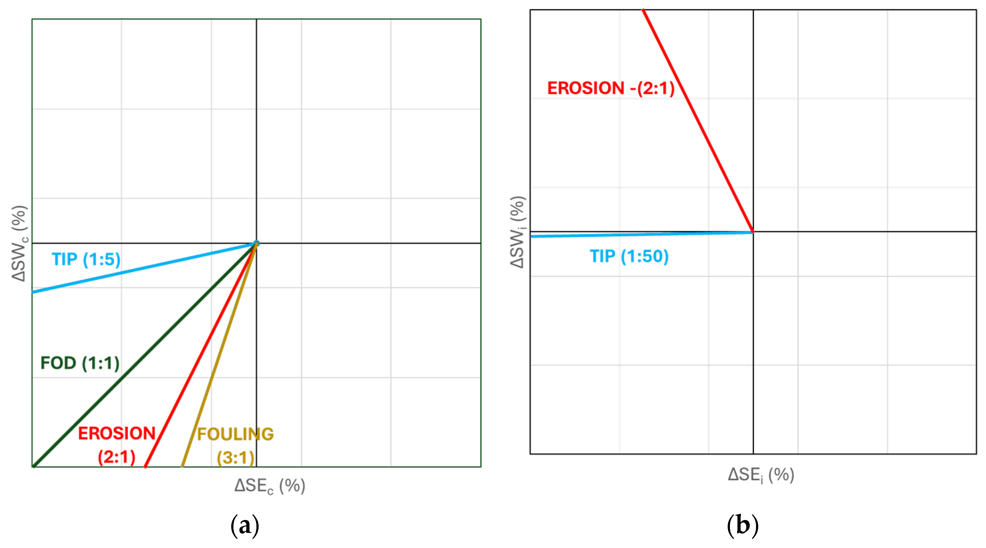
  • The ratio of ΔSWc and ΔSEc is found:
    Δ S W c Δ S E c = r
  • The calculated ratio ‘r’ is compared with the ratios of the considered faults of the affected component from the knowledge base. The fault with the closest ratio is the one that is present.

4. Application to a Mixed Flow Turbofan

The procedure described above is elucidated through application to a mixed-flow turbofan engine, with a configuration similar to those in civil aviation service today. In this application, simulated values of the input measurements were considered.

4.1. Engine Description

A layout of the considered engine is shown in Figure 4, including station numbering, the position of available measurements, and relevant health parameters.
The measurements and health parameters that form vectors u, f, and Y are summarized in Table 1.
A performance model (EPM) has been developed for this engine and is used to generate the Jacobian matrix. A deviation magnitude Δ f = 3% is used for this purpose. The considered EPM relies on a state-of-the-art approach, first presented in [44] and further developed ever since, achieving high-accuracy simulations compared with other industry-accepted models [44], as well as on actual stationary engine data [18] and aircraft engine data [38].
The considered engine comprises four components; thus, the PNN is built with five output classes, as described in Table 2. The threshold for healthy operation is chosen as h = 0.5%.

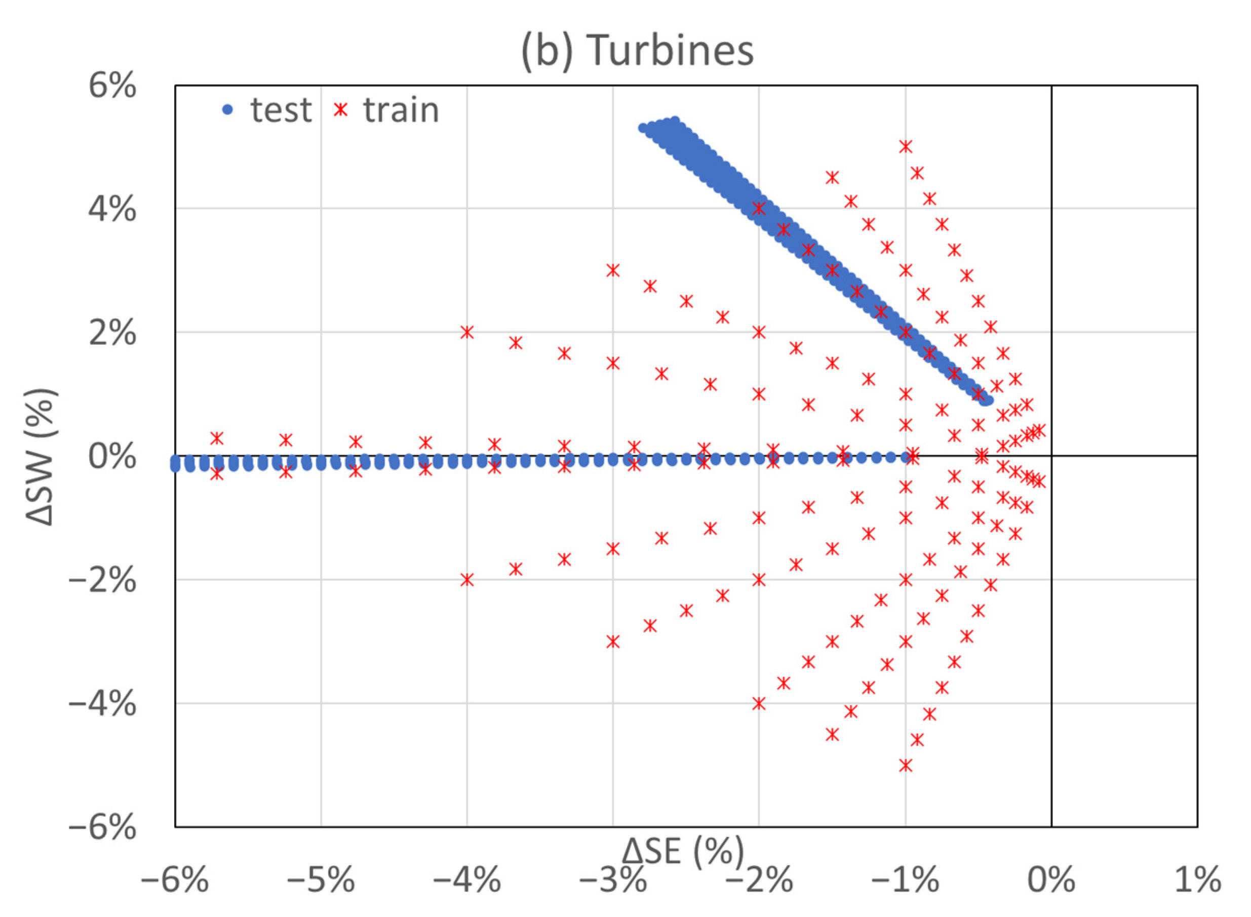
4.2. PNN Testing–Τraining Patterns

To evaluate the effectiveness of the diagnostic method, test patterns that cover a set of faults considered are generated. The faults of all components were considered, and various magnitudes and ratios around the value representing that fault were included. Table A2 in Appendix A summarizes the engine health conditions of the test cases, expressed in terms of fault magnitudes and ratios.
The PNN is equipped with the capability to generate training patterns, as explained previously. Patterns where no health parameter deviates more than ±0.5% and patterns of various ratios and magnitudes for each component, representing various types and severities of faults, are included. Table A1 summarizes the deviations considered in health parameters for generating training patterns for each class. It should be noted that training patterns cover not only deviations corresponding to the particular faults considered but also additional deviating situations, even though they do not correspond to the actual faults of interest. The deviation ratios for these faults are introduced in the knowledge base and are used to identify the type of fault in the last step of the method.
Figure 5 shows health conditions (i.e., health parameter deviations) for the generation of both training and testing patterns in the corresponding component diagnostic plane (ΔSW versus ΔSE). The training patterns (red marks) cover the entire space of possible deviations of the health parameters. The fault space thus covered includes the examined faults, which correspond to the directions shown on the diagnostic plane, Figure 1, but extends to faulty situations that would cover the entire diagnostic plane, even though some of the combinations do not correspond to known faults. This coverage of the fault space was found to maximize the effectiveness of the PNN in determining the faulty component. The combinations used to generate test patterns (blue marks) include different ratios and magnitudes, encompassing the direction for the nominal ratio for this fault. This distribution is chosen to cover possible scattering of values when actual measurement data are used.
The Engine Performance Model is used for data generation. All simulated measurement values are contaminated with noise. The noise levels used are typical for this kind of instrumentation and are listed in Appendix B, Table A4.
For all fault cases, data were generated at 18 operating points (OP), covering the entire flight envelope of the engine (see Table A3).

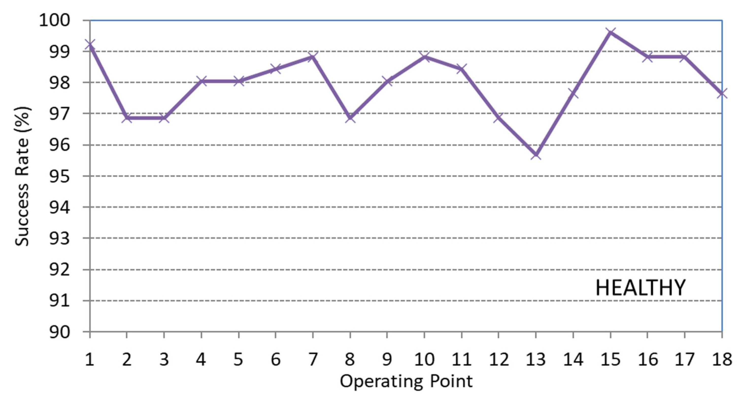
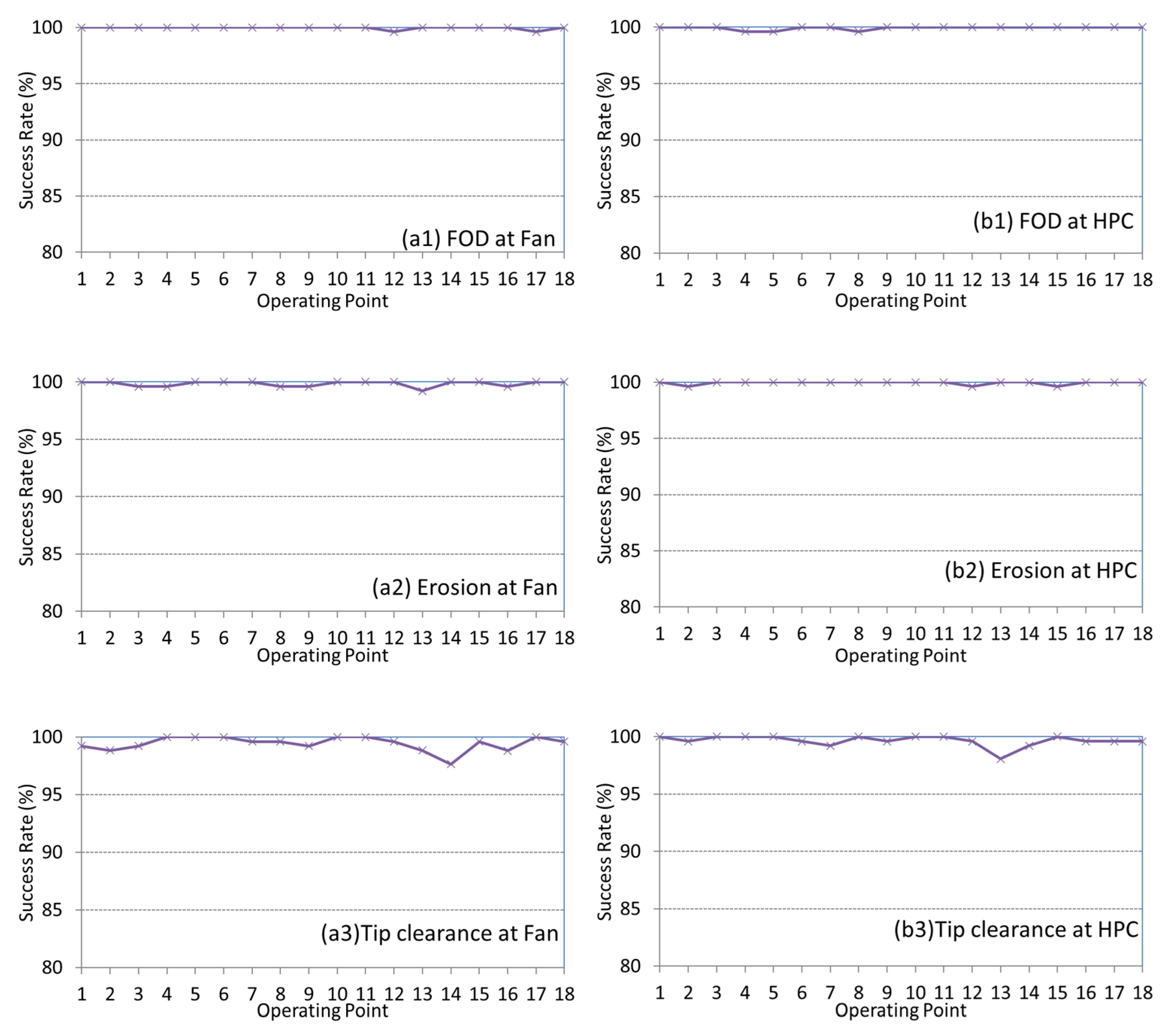
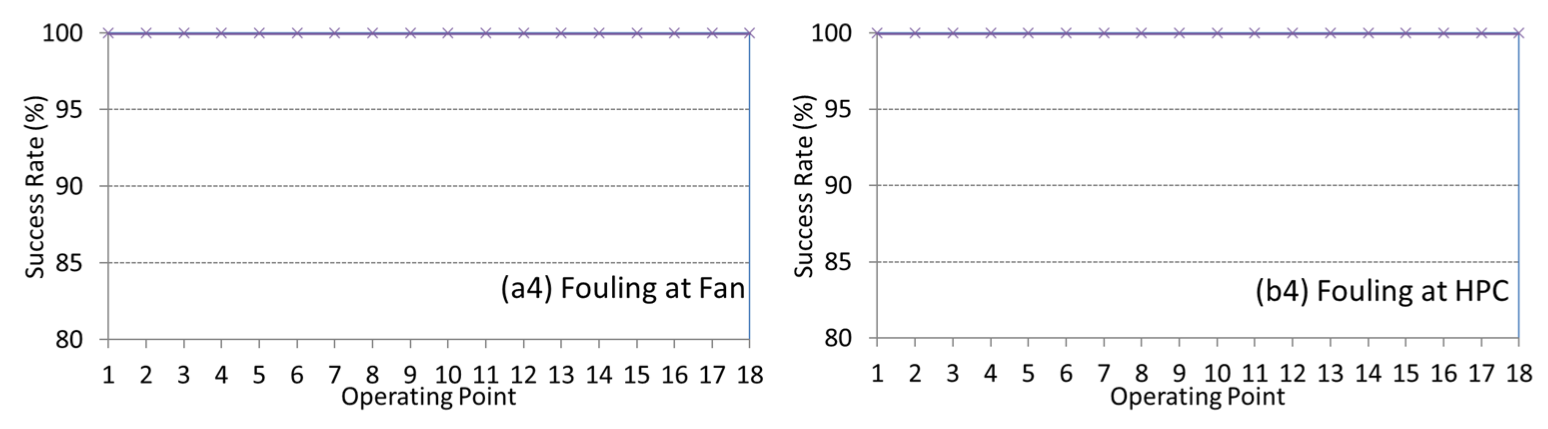
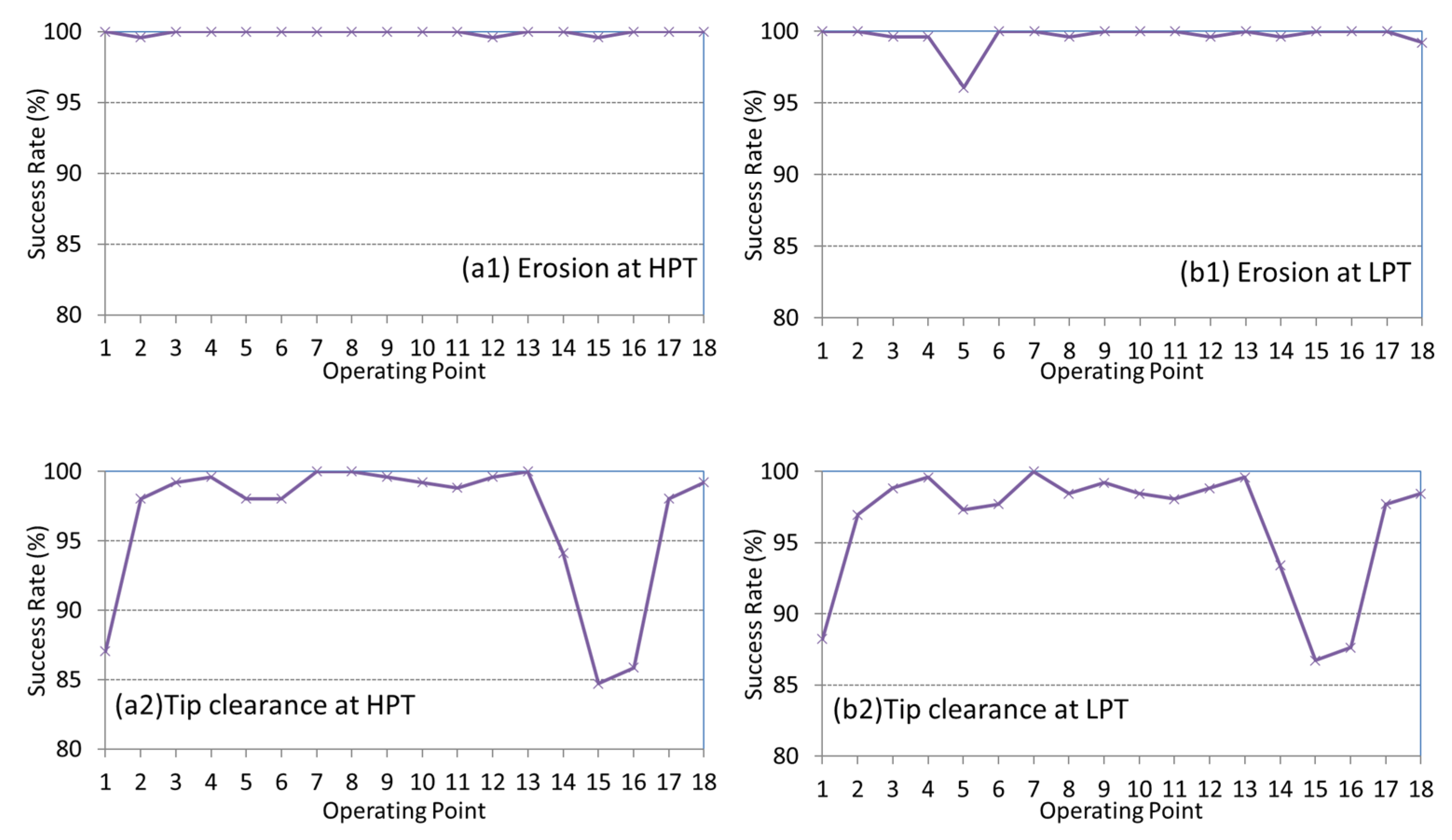
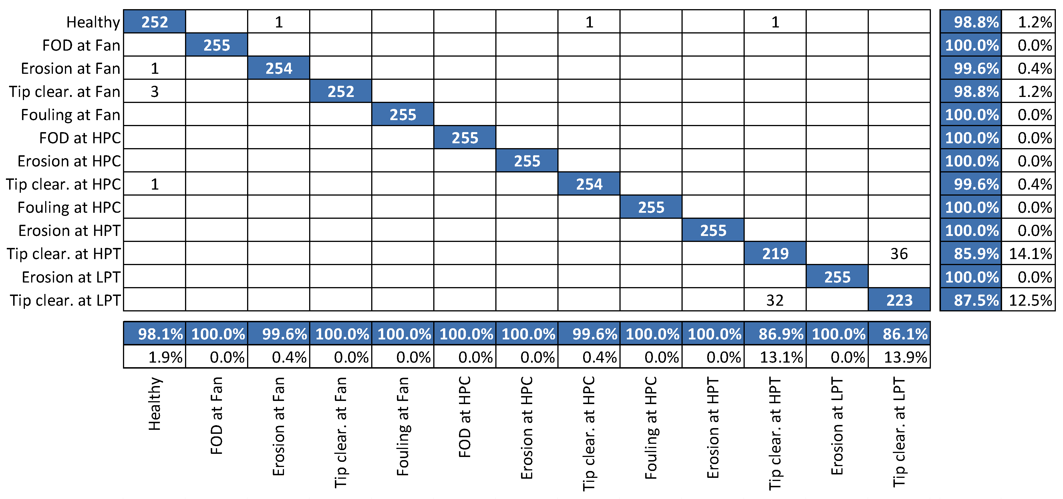
4.3. Diagnostic Method Efficiency

The effectiveness of the proposed method is assessed by producing diagnoses for different cases and then evaluating the statistics of the obtained results. For each operating point and health condition, the overall performance is expressed in terms of the success rate, which is defined as follows:
S u c c e s s   R a t e   % = N Ν t o t a l · 100 %
N is the number of examined test cases of a specific health condition at a specific operating point where the existing physical fault is detected correctly. Ν t o t a l is the total number of examined test cases of a specific health condition at a specific operating point, 255 in our case, as described in Table A2. In the case of healthy engine operation, N is the number of examined test cases in which the applied diagnostic method concluded that no fault occurs (healthy operation of the engine).
Figure 6 shows the success rates of the considered diagnostic method for HEALTHY test cases. As can be seen, the success rate ranges from more than 95% to 100%, depending on the operating point.
Figure 7 shows the success rates of the diagnostic method for the compressor faults test cases (FAN and HPC). As can be seen, the success rate ranges from 98% to 100%, depending on the operating point.
Figure 8 shows the success rates of the diagnostic method for the turbine faults test cases (HPT and LPT). As can be seen, the success rate ranges from 96% to 100% in almost all cases. There are, however, 3 low-power operating points (OP ID. 1, 15, and 16) of the tip clearance fault cases at which the diagnostic method has a lower performance of around 84% to 88%.
A closer look at the behavior of the diagnostic method can be obtained using the corresponding confusion matrix. A confusion matrix is a commonly accepted performance evaluation tool in machine learning that represents the accuracy of a classification model [45]. The confusion matrix for the test patterns at OP with ID 16 is shown in Figure 9.
Each line of the matrix shows to which faults (noted at the bottom of the table) the test patterns of a specific fault (noted at the left) are attributed. The two cells at the far right provide the score for correct and incorrect classification. The diagonal elements contain the number of correctly classified patterns. For instance, line 4 of the confusion matrix indicates that the diagnostic method correctly identified 252 test patterns of tip clearance faults at the FAN, and 3 test patterns were misclassified as HEALTHY cases. This is translated into a 98.8% correct diagnosis and 1.2% misdiagnosis. Thus, each column shows how many test patterns of a specific fault (noted at the left) are detected as the fault noted at the bottom of the table. The two cells at the far bottom provide the score of correct classification and misclassification. For instance, column 3 of the confusion matrix indicates that the diagnostic method correctly identified 254 test patterns of erosion faults at the FAN, and 1 healthy test pattern was misclassified as erosion at the FAN. This is translated into a 99.6% correct diagnosis and 0.4% misdiagnosis.
As seen in this confusion matrix, out of the 255 tip clearance fault cases at the HPT examined, 219 were identified correctly (success rate 85.9%). In contrast, the remaining 36 cases (14.1% of cases) were misdiagnosed as tip clearance faults in the LPT. It seems, therefore, that regarding tip clearance faults at the HPT, there is confusion about the location of the fault in the correct turbine. This confusion, although not very extensive according to the considered test set, can be explained by the lack of an additional interturbine measurement that could distinguish faults between the two turbines.
The above procedure can be applied to assess other diagnostic method configurations. For example, the PNN can be configured with output classes for individual component faults in the first step of the diagnostic method. On the other hand, the PNN could be configured to constitute a single-step diagnostic method by including additional classes that categorize the magnitude of fault without evoking the estimation of step 2 of the current approach. The authors have considered various alternative PNN configurations, with the one presented here performing better, even though the difference in performance was insignificant.

5. Discussion

The effectiveness of the proposed diagnostic method was tested in detecting and identifying single-component faults. It should be assessed by an interested user from this perspective. However, since it is a two-step approach—first detecting the faulty component and then determining the magnitude of the component health parameter deviations—it could also be considered for multiple fault identification. Although not covered here, approaches for performing such an exercise can be considered (e.g., sorting probabilities of component faults); however, this is clearly the subject of future work and is not covered here.
The key feature of the proposed method is the dynamic generation of training information at specific operating conditions, where test data are collected. This is crucial for turbofans, which operate under various conditions within a single aircraft mission. At the early stages of their work on PNN [46], the authors have already demonstrated that detection accuracy is reduced when training data include sets generated at operating conditions other than those in which test data have been collected. This behavior was also confirmed during the development of the present method. A ‘conventional’ PNN, fed with training information generated a priori, namely signatures from multiple operating conditions covering a flight envelope, was tested. Its performance was inferior to that of the proposed dynamic PNN, with reduced success rates that can be as much as 10% lower for turbine faults.
The generation of training information at the operating conditions from which the test data come inherently tackles the problem of data scarcity. Methods based on a priori-generated training data may face a scarcity situation if the training data do not cover a particular operating condition encountered during a flight. Such situations do not occur with the proposed method, as the training set is generated at the same operating conditions as the test data, with adequate coverage of the fault space (as discussed in Section 4.2 above). The only requirement is that the EPM is adapted to the monitored engine. Information about building adapted models in real-life cases can be found in [15,16,38].
A question that may arise is how the effectiveness of the present method is compared with other diagnostic methods for the same purpose; however, again, this is the subject of further work. Comparisons of methods have been the subject of various publications (e.g., [1,2,3,4,5,6,7,8,9]). To illustrate the importance of careful comparisons, an international benchmark exercise organized by NASA [46], under the name ‘Propulsion Diagnostic Method Evaluation Strategy’ (ProDiMES), is mentioned here. The authors have participated in this exercise [47] and tested the effectiveness of six diagnostic methods in the ProDiMES environment. A PNN was found to be the top performer for single-fault identification. In any case, the distinct advantages of PNNs, as presented by Specht [33] in his publication introducing the form of PNN used in this paper, are recalled.
Another question could be posed about the robustness of the proposed method to the noise level in the measured data. PNNs are known to be quite robust to noise, which was verified by the test data presented here. A situation with increased noise level was considered: the measurement vector fed to the PNN for testing each considered case was derived by averaging 10 records from the simulated raw acquired data instead of the 100 used for the previously reported tests. The inputs to the PNN thus exhibited an increased noise level. The success rates for each examined fault, considering all 18 operating points, are summarized in Table 3.
It can be seen that the performance of the PNN degrades by small amounts, even though the noise has increased significantly, confirming the performance expected from this type of network. We note that an exhaustive study of the effects of noise on the performance of the proposed method was not the subject of the present work. The focus was on situations representative of real-life conditions in turbofan operation. A detailed study of such effects can be conducted if a specific noise situation is of practical interest.
The diagnostic method presented can be executed in ‘real time’. Although an Engine Performance Model is used to generate training patterns, employing the Jacobian matrix ensures efficient execution. The PNN, on the other hand, operates almost instantaneously. For example, generating a PNN for one operating condition requires approximately a second on a contemporary PC, while executing the PNN requires less than a millisecond.

6. Conclusions

A diagnostic method for gas-path faults in gas turbines has been presented utilizing a Probabilistic Neural Network (PNN) coupled with an Engine Performance Model. The proposed method allows diagnosis using a compact knowledge base generated from physical information about component faults, unlike conventional approaches that require a large amount of measurement signature information to support the PNN. Moreover, coupling with the Engine Performance Model allows the achievement of a more robust diagnosis, as the large variability in engine operating conditions inherent to aircraft engines is directly addressed, again with no need for extensive training datasets.
An efficient two-step approach is followed, with an estimation algorithm that allows a precise determination of the magnitude of the fault present in a component once the PNN has detected its presence.
The performance of the proposed method was examined against realistic data of some of the most common faults (i.e., fouling, FOD, erosion, and tip clearance) at the compressor and turbines of a mixed-flow turbofan engine operating under various conditions in a flight envelope.
The diagnostic results demonstrate that the proposed method is a simple yet efficient diagnostic tool.

Author Contributions

Conceptualization, N.A., C.R. and K.M.; investigation, N.A. and C.R.; supervision, K.M.; data curation, N.A., C.R. and K.M.; writing—original draft preparation, C.R.; writing—review and editing, K.M. All authors have read and agreed to the published version of the manuscript.

Funding

This research was performed under subcontract to Delta System Solutions GmbH for a contract funded by the Agency for Development of Defense, Republic of Korea (U22038JF).

Data Availability Statement

The data presented in this study are openly available in the open literature cited and reported in the dedicated references section.

Conflicts of Interest

The authors declare no conflicts of interest.

Appendix A. Description of Training and Testing Patterns

Table A1 summarizes the health parameter deviations for the generation of training patterns for each class of the PNN representing an engine component fault. They correspond to the red symbols in Figure 5. In this table, the considered fault magnitudes (L) and fault ratios tan(θ), which were defined using Equations (9) and (10) for each component, are shown, together with the total number of training patterns of the corresponding class. The set of faults considered for training at any component results from all possible combinations of 26 (in total) different fault magnitudes (L) with the 6 different fault ratios of the component’s health parameters; thus, we obtain a total of 26 × 6 = 156 training patterns per class, which represents an engine component fault. The selected ratios and fault magnitudes provide fair coverage of the fault range that may occur at any component.
For the ‘HEALTHY’ class’s 156 training patterns, a random deviation of all health parameters was considered, assuming that this deviation is normally distributed around 0% with σ = 0.1%.
Table A1. Sets of fault magnitudes and ratios used to generate training patterns for each class that represent engine component faults. Deviation values are in percentages.
Fault Magnitudes (L)Fault Ratios (tan(θ))No. of Training Patterns
−[0.5, 1.0, 1.5, 2.0, 2.5, 3.0, 3.5,
4.0, 4.5, 5.0, 5.5, 6.0, 30]
+[0.05, 0.5, 1, 2, 3, 5]13 × 12 = 156
+[0.5, 1.0, 1.5, 2.0, 2.5, 3.0, 3.5,
4.0, 4.5, 5.0, 5.5, 6.0, 30]
−[0.05, 0.5, 1, 2, 3, 5]
The sets used to generate testing patterns are listed in Table A2. They correspond to the blue symbols in Figure 5. For instance, the second row of the table describes the considered tip clearance fault cases of the Fan. Each such case results in a deviation of SW2 and SE2, at a ratio that varies from 0.4 to 0.6, at a step of 0.05 (total number of ratios considered: [(0.6 − 0.4)/0.05] + 1 = 5). For each ratio, several severities of the fault have been considered, expressed in several fault magnitudes that vary from −1 to −6, at a step of 0.1 (total number of fault magnitudes considered: [(6 − 1)/0.1] + 1 = 51). This resulted in some 51 × 5 = 255 test cases for this type of fault. Similarly, the considered test cases for the remaining faults are shown in this table. The severity of the faults examined, as expressed by the magnitude of the deviations in the health parameters, is based on experience documented in many published gas turbine fault cases, as also reviewed by the authors in [11].
Table A2. Sets of fault magnitudes and ratios used for the generation of test patterns.
ComponentFaultFault Magnitudes (L)Fault Ratios (tan(θ))No. of
Test Patterns
FromToStepFromToStep
NoneNo fault00N/AN/A255
FANTip clearance−1−60.10.40.60.0551 × 5 = 255
FANErosion−1−60.11.92.10.0551 × 5 = 255
FANFOD−1−60.10.91.10.0551 × 5 = 255
FANFouling−1−60.1−2.9−3.10.0551 × 5 = 255
HPCTip clearance−1−60.10.10.30.0551 × 5 = 255
HPCErosion−1−60.11.92.10.0551 × 5 = 255
HPCFOD−1−60.10.91.10.0551 × 5 = 255
HPCFouling−1−60.1−2.9−3.10.0551 × 5 = 255
HPTTip clearance−1−60.10.010.030.0551 × 5 = 255
HPTErosion160.1−1.9−2.10.0551 × 5 = 255
LPTTip clearance−1−60.10.010.030.0551 × 5 = 255
LPTErosion160.1−1.9−2.10.0551 × 5 = 255

Appendix B. Considered Operating Points and Measurement Noise of the Available Instrumentation

The faults created for testing the effectiveness of the method were generated at a number of different engine operating points (OP), providing a representative coverage of conditions over the entire flight envelope. Eighteen operating points were considered, as presented in Table A3, in terms of altitude (Alt), temperature difference from ISA (dTisa), flight Mach number (M), and corrected low-pressure shaft speed (N1corr). They include operation at ground level, at a speed setting close to idle, start of ground run and takeoff, flight at a medium and a high altitude with different cruising speeds, and lower speed settings representative of approach conditions.
Table A3. Considered operating points of the examined test cases.
OP idAlt (ft)dTisaMN1cor (%)
100035
2000100
35000.2100
445,00000.6100
545,00000.695
645,00000.895
745,00000.890
845,00000.690
945,00000.680
1025,00000.680
1125,00000.6100
1245,00000.8100
1345,00000.890
1445,00000.850
155000.250
165000.235
1700098.12
1835,000100.8100
From Table A2 and Table A3, it is evident that the test set consists of a total number of
255 (test cases per health condition and OP) × 13 (health conditions) × 18 (OP) = 59.670 (test cases)
Table A4 summarizes the available measurements, their symbolic names, and the associated noise levels. The noise levels are expressed in standard deviation as a percentage of the measured values. The measured quantities and noise levels are typical of actual turbofans in operation, as discussed in [36].
Table A4. Measurements available for diagnosis and associated noise levels.
MeasurementSymbolNoise (%)
Ambient pressurePamb0.14
Total pressure at station ‘0’Pt00.10
Total temperature at station ‘0’Tt00.23
LP shaft speedNL0.05
Fuel flow rateWf0.15
HP shaft speedNH0.05
Total pressure at station ‘13’Pt130.17
Total temperature at station ‘13’Tt130.23
Total pressure at station ‘31’Pt310.17
Total temperature at station ‘31’Tt310.10
Total temperature at station ‘5’Tt50.10
Total pressure at station ‘45’Pt450.17
For each fault case at an operating condition, 100 vectors of measurements were generated with the aid of the EPM and were contaminated with noise. The vector presented in the diagnostic method is derived as the average of these 100 vectors of measurements. This replicates how modern aircraft data acquisition systems operate to reduce the effect of measurement noise.

References

  1. Fentaye, A.D.; Gilani, S.I.U.-H.; Baheta, A.T. Gas Turbine Gas Path Diagnostics: A Review. MATEC Web Conf. 2016, 74, 00005. [Google Scholar] [CrossRef]
  2. Vu, D.Q.; Razakarivony, S.; Marnissi, Y.; Nocture, M. A Comprehensive Literature Review on the Resolution of Turbine Engine Performances’ Inverse Problems. In Volume 4: Controls, Diagnostics, and Instrumentation, Proceedings of the ASME Turbo Expo 2024: Turbomachinery Technical Conference and Exposition, London, UK, 24–28 June 2024; American Society of Mechanical Engineers: New York, NY, USA, 2024; p. V004T05A045. [Google Scholar]
  3. Fentaye, A.D.; Baheta, A.T.; Gilani, S.I.; Kyprianidis, K.G. A Review on Gas Turbine Gas-Path Diagnostics: State-of-the-Art Methods, Challenges and Opportunities. Aerospace 2019, 6, 83. [Google Scholar] [CrossRef]
  4. Hanachi, H.; Mechefske, C.; Liu, J.; Banerjee, A.; Chen, Y. Performance-Based Gas Turbine Health Monitoring, Diagnostics, and Prognostics: A Survey. IEEE Trans. Reliab. 2018, 67, 1340–1363. [Google Scholar] [CrossRef]
  5. Tahan, M.; Tsoutsanis, E.; Muhammad, M.; Abdul Karim, Z.A. Performance-Based Health Monitoring, Diagnostics and Prognostics for Condition-Based Maintenance of Gas Turbines: A Review. Appl. Energy 2017, 198, 122–144. [Google Scholar] [CrossRef]
  6. De Castro-Cros, M.; Velasco, M.; Angulo, C. Machine-Learning-Based Condition Assessment of Gas Turbines—A Review. Energies 2021, 14, 8468. [Google Scholar] [CrossRef]
  7. Le Clainche, S.; Ferrer, E.; Gibson, S.; Cross, E.; Parente, A.; Vinuesa, R. Improving Aircraft Performance Using Machine Learning: A Review. Aerosp. Sci. Technol. 2023, 138, 108354. [Google Scholar] [CrossRef]
  8. Liu, X.; Chen, Y.; Xiong, L.; Wang, J.; Luo, C.; Zhang, L.; Wang, K. Intelligent Fault Diagnosis Methods toward Gas Turbine: A Review. Chin. J. Aeronaut. 2024, 37, 93–120. [Google Scholar] [CrossRef]
  9. Hashmi, M.B.; Fentaye, A.D.; Mansouri, M.; Kyprianidis, K.G. A Comparative Analysis of Various Machine Learning Approaches for Fault Diagnostics of Hydrogen Fueled Gas Turbines. In Volume 4: Controls, Diagnostics, and Instrumentation, Proceedings of the ASME Turbo Expo 2024: Turbomachinery Technical Conference and Exposition, London, UK, 24–28 June 2024; American Society of Mechanical Engineers: New York, NY, USA, 2024; p. V004T05A050. [Google Scholar]
  10. Zhou, D.; Huang, D. A Review on the Progress, Challenges and Prospects in the Modeling, Simulation, Control and Diagnosis of Thermodynamic Systems. Adv. Eng. Inform. 2024, 60, 102435. [Google Scholar] [CrossRef]
  11. Mathioudakis, K.; Alexiou, A.; Aretakis, N.; Romesis, C. Signatures of Compressor and Turbine Faults in Gas Turbine Performance Diagnostics: A Review. Energies 2024, 17, 3409. [Google Scholar] [CrossRef]
  12. Urban, L.A. Gas Turbine Engine Parameter Interrelationships, 2nd ed.; HSD UTC: Windsor Locks, CT, USA, 1969. [Google Scholar]
  13. Urban, L.A.; Volponi, A.J. Mathematical Methods of Relative Engine Performance Diagnostics; SAE International: Warrendale, PA, USA, 1992; p. 922048. [Google Scholar]
  14. Doel, D. TEMPER—A Gas Path Analysis Tool for Commercial Jet Engines. J. Eng. Gas Turbines Power 1994, 116, 82–89. [Google Scholar] [CrossRef]
  15. Stamatis, A.; Mathioudakis, K.; Papailiou, K.D. Adaptive Simulation of Gas Turbine Performance. J. Eng. Gas Turbine Power 1990, 112, 168–175. [Google Scholar] [CrossRef]
  16. Li, Y.G. Gas Turbine Performance and Health Status Estimation Using Adaptive Gas Path Analysis. J. Eng. Gas Turbines Power 2010, 132, 041701. [Google Scholar] [CrossRef]
  17. Aretakis, N.; Roumeliotis, I.; Mathioudakis, K. Performance Model “Zooming” for In-Depth Component Fault Diagnosis. J. Eng. Gas Turbines Power 2011, 133, 031602. [Google Scholar] [CrossRef]
  18. Roumeliotis, I.; Aretakis, N.; Alexiou, A. Industrial Gas Turbine Health and Performance Assessment with Field Data. J. Eng. Gas Turbines Power 2017, 139, 051202. [Google Scholar] [CrossRef]
  19. Aretakis, N.; Mathioudakis, K.; Stamatis, A. Identification of Sensor Faults on Turbofan Engines Using Pattern Recognition Techniques. Control Eng. Pract. 2004, 12, 827–836. [Google Scholar] [CrossRef]
  20. Bunks, C.; Mccarthy, D.; Al-Ani, T. Condition-based maintenance of machines using hidden markov models. Mech. Syst. Signal Process. 2000, 14, 597–612. [Google Scholar] [CrossRef]
  21. Nadir, F.; Elias, H.; Messaoud, B. Diagnosis of Defects by Principal Component Analysis of a Gas Turbine. SN Appl. Sci. 2020, 2, 980. [Google Scholar] [CrossRef]
  22. Allen, C.W.; Holcomb, C.M.; De Oliveira, M. Gas Turbine Machinery Diagnostics: A Brief Review and a Sample Application. In Volume 6: Ceramics; Controls, Diagnostics and Instrumentation; Education, Proceedings of the ASME Turbo Expo 2017: Turbomachinery Technical Conference and Exposition, Charlotte, NC, USA, 26–30 June 2017; Manufacturing Materials and Metallurgy; American Society of Mechanical Engineers: New York, NY, USA, 2017; p. V006T05A028. [Google Scholar]
  23. Luo, H.; Zhong, S. Gas Turbine Engine Gas Path Anomaly Detection Using Deep Learning with Gaussian Distribution. In Proceedings of the 2017 Prognostics and System Health Management Conference (PHM-Harbin), Harbin, China, 9–12 July 2017; IEEE: Piscataway, NJ, USA, 2017; pp. 1–6. [Google Scholar]
  24. Tamilselvan, P.; Wang, P. Failure Diagnosis Using Deep Belief Learning Based Health State Classification. Reliab. Eng. Syst. Saf. 2013, 115, 124–135. [Google Scholar] [CrossRef]
  25. Zhao, Y.-P.; Wang, J.-J.; Li, X.-Y.; Peng, G.-J.; Yang, Z. Extended Least Squares Support Vector Machine with Applications to Fault Diagnosis of Aircraft Engine. ISA Trans. 2020, 97, 189–201. [Google Scholar] [CrossRef]
  26. Zhou, D.; Yao, Q.; Wu, H.; Ma, S.; Zhang, H. Fault Diagnosis of Gas Turbine Based on Partly Interpretable Convolutional Neural Networks. Energy 2020, 200, 117467. [Google Scholar] [CrossRef]
  27. Cao, Q.; Chen, S.; Zheng, Y.; Ding, Y.; Tang, Y.; Huang, Q.; Wang, K.; Xiang, W. Classification and Prediction of Gas Turbine Gas Path Degradation Based on Deep Neural Networks. Int. J. Energy Res. 2021, 45, 10513–10526. [Google Scholar] [CrossRef]
  28. Zhao, J.; Li, Y.G. Abrupt Fault Detection and Isolation for Gas Turbine Components Based on a 1D Convolutional Neural Network Using Time Series Data. In Proceedings of the AIAA Propulsion and Energy 2020 Forum, Virtual Event, 24–26 August 2020; American Institute of Aeronautics and Astronautics: Reston, VA, USA, 2020. [Google Scholar]
  29. Amare, F.D.; Gilani, S.I.; Aklilu, B.T.; Mojahid, A. Two-Shaft Stationary Gas Turbine Engine Gas Path Diagnostics Using Fuzzy Logic. J. Mech. Sci. Technol. 2017, 31, 5593–5602. [Google Scholar] [CrossRef]
  30. Wang, X.-X.; Ma, L.-Y. A Compact K Nearest Neighbor Classification for Power Plant Fault Diagnosis. J. Inf. Hiding Multimed. Signal Process. 2014, 5, 508–517. [Google Scholar]
  31. Romessis, C.; Mathioudakis, K. Bayesian Network Approach for Gas Path Fault Diagnosis. J. Eng. Gas Turbines Power 2006, 128, 64–72. [Google Scholar] [CrossRef]
  32. Bose, N.K.; Liang, P. Neural Network Fundamentals with Graphs, Algorithms and Applications; McGraw-Hill Series in Electrical and Computer Engineering; McGraw-Hill: New York, NY, USA, 1996; ISBN 978-0-07-006618-2. [Google Scholar]
  33. Specht, D.F. Probabilistic neural networks. Neural Netw. 1990, 3, 109–118. [Google Scholar] [CrossRef]
  34. Mohebali, B.; Tahmassebi, A.; Meyer-Baese, A.; Gandomi, A.H. Chapter 14—Probabilistic neural networks: A brief overview of theory, implementation, and application. In Handbook of Probabilistic Models; Butterworth-Heinemann: Oxford, UK, 2020; pp. 347–367. ISBN 9780128165140. [Google Scholar] [CrossRef]
  35. Eustace, R.; Merrington, G. Fault Diagnosis of Fleet Engines Using Neural Networks. In Proceedings of the Twelfth International Symposium on Air Breathing Engines, Melbourne, Australia, 10–15 September 1995. paper no. ISABE 95-7085. [Google Scholar]
  36. Romesis, C.; Mathioudakis, K. Setting Up of a Probabilistic Neural Network for Sensor Fault Detection Including Operation with Component Faults. J. Eng. Gas Turbines Power 2003, 125, 634–641. [Google Scholar] [CrossRef]
  37. Romessis, C.; Stamatis, A.; Mathioudakis, K. A Parametric Investigation of the Diagnostic Ability of Probabilistic Neural Networks on Turbofan Engines. In Volume 4: Manufacturing Materials and Metallurgy; Ceramics; Structures and Dynamics; Controls, Diagnostics and Instrumentation; Education; IGTI Scholar Award, Proceedings of the ASME Turbo Expo 2001: Power for Land, Sea, and Air, New Orleans, Louisiana, USA, 4–7 June 2001; American Society of Mechanical Engineers: New York, NY, USA, 2001; p. V004T04A004. [Google Scholar]
  38. Aretakis, N.; Roumeliotis, I.; Alexiou, A.; Romesis, C.; Mathioudakis, K. Turbofan Engine Health Assessment From Flight Data. J. Eng. Gas Turbines Power 2015, 137, 041203. [Google Scholar] [CrossRef]
  39. Romessis, C.; Mathioudakis, K. Implementation of Stochastic Methods for Industrial Gas Turbine Fault Diagnosis. In Volume 1: Turbo Expo 2005, Proceedings of the ASME Turbo Expo 2005: Power for Land, Sea, and Air, Reno, NV, USA, 6–9 June 2005; ASMEDC: New York, NY, USA, 2005; pp. 723–730. [Google Scholar]
  40. Butler, S.W.; Pattipati, K.R.; Volponi, A.; Hull, J.; Rajamani, R.; Siegel, J. An Assessment Methodology for Data-Driven and Model-Based Techniques for Engine Health Monitoring. In Volume 2: Aircraft Engine; Ceramics; Coal, Biomass and Alternative Fuels; Controls, Diagnostics and Instrumentation; Environmental and Regulatory Affairs, Proceedings of the ASME Turbo Expo 2006: Power for Land, Sea, and Air, Barcelona, Spain, 8–11 May 2006; ASMEDC: New York, NY, USA, 2006; pp. 823–831. [Google Scholar]
  41. Jiang, R.; Zhu, W. A PNN fault diagnosis method for gas turbine. In Proceedings of the World Automation Congress 2012, Puerto Vallarta, Mexico, 24–28 June 2012; pp. 1–4. [Google Scholar]
  42. Loboda, I.; Olivares Robles, M.A. Gas Turbine Fault Diagnosis Using Probabilistic Neural Networks. Int. J. Turbo Jet-Engines 2015, 32, 175–191. [Google Scholar] [CrossRef]
  43. Cao, Y.; Lv, X.; Han, G.; Luan, J.; Li, S. Research on Gas-Path Fault-Diagnosis Method of Marine Gas Turbine Based on Exergy Loss and Probabilistic Neural Network. Energies 2019, 12, 4701. [Google Scholar] [CrossRef]
  44. Alexiou, A.; Mathioudakis, K. Development of Gas Turbine Performance Models Using a Generic Simulation Tool. In Proceedings of the ASME Turbo Expo 2005, Reno, NV, USA, 6–9 June 2005; ASME: New York, NY, USA, 2005; pp. 185–194. [Google Scholar] [CrossRef]
  45. Fawcett, T. An Introduction to ROC Analysis. Pattern Recognit. Lett. 2006, 27, 861–874. [Google Scholar] [CrossRef]
  46. Simon, D.L.; Borguet, S.; Leonard, O.; Zhang, X. Aircraft Engine Gas Path Diagnostic Methods: Public Benchmarking Results. J. Eng. Gas Turbines Power 2013, 136, 041201. [Google Scholar] [CrossRef]
  47. Koskoletos, O.; Aretakis, N.; Alexiou, A. Evaluation of Aircraft Engine Diagnostic Methods through ProDiMES. In Proceedings of the ASME Turbo Expo 2018: Turbomachinery Technical Conference and Exposition, Oslo, Norway, 11–15 June 2018. [Google Scholar]
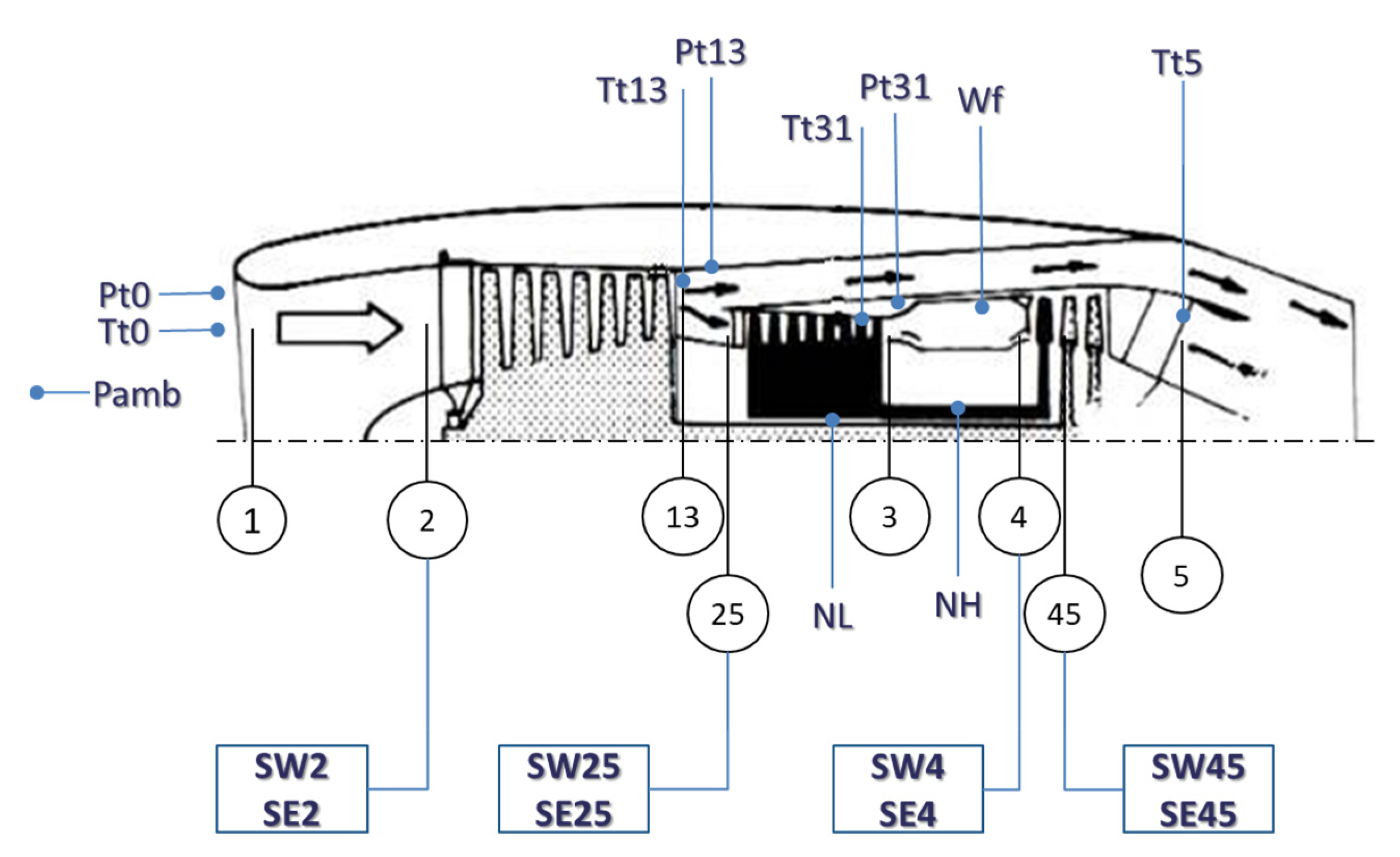
Figure 1. Mapping the faults considered on the diagnostic plane and their association to ratios of health parameters deviations (Δ SW c S E c ) of the affected component: (a) compressor, (b) turbine.
Aerospace 11 00913 g001
Figure 2. Overview of the proposed diagnostic method scheme.
Aerospace 11 00913 g002
Figure 3. Cross-plot of a component’s deviations of health parameters, introducing the formation of the knowledge base of the diagnostic method.
Aerospace 11 00913 g003
Figure 4. The layout of the engine, showing measurements and parameters involved.
Aerospace 11 00913 g004
Figure 5. Cross-plot training vs test patterns of faults in (a) compressors and (b) turbines.
Aerospace 11 00913 g005aAerospace 11 00913 g005b
Figure 6. Success rates of the diagnostic method, under all considered operating points, at HEALTHY test cases.
Aerospace 11 00913 g006
Figure 7. Success rates of the diagnostic method under all considered operating points for FAN and HPC test cases.
Aerospace 11 00913 g007aAerospace 11 00913 g007b
Figure 8. Success rates of the diagnostic method, under all considered operating points, at HPT and LPT test cases.
Aerospace 11 00913 g008
Figure 9. The confusion matrix of the diagnostic method on the test patterns at OP with ID 16.
Aerospace 11 00913 g009
Table 1. Available measurements and considered health parameters.
uSymbolfSymbol
Ambient pressurePambFAN Flow factorSW2
Total pressure at station ‘0’Pt0FAN Efficiency factorSE2
Total temperature at station ‘0’Tt0HPC Flow factorSW25
LP shaft speedNLHPC Efficiency factorSE25
YSymbolHPT Flow factorSW4
Fuel flow rateWfHPT Efficiency factorSE4
HP shaft speedNHLPT Flow factorSW45
Total pressure at station ‘13’Pt13LPT Efficiency factorSE45
Total temperature at station ‘13’Tt13
Total pressure at station ‘31’Pt31
Total temperature at station ‘31’Tt31
Total temperature at station ‘5’Tt5
Table 2. The PNN classes for the application of the diagnostic method.
Class No.Class SymbolClass Description
1HEALTHYHealthy condition. All |ΔSW|, |ΔSE| ≤ 0.5%
2FANFault only in the FAN. |ΔSW2|, |ΔSE2| > 0.5%,
3HPCFault only in the HPC. |ΔSW25|, |ΔSE25| > 0.5%,
4HPTFault only in the HPT. |ΔSW4|, |ΔSE4| > 0.5%,
5LPTFault only in the LPT. |ΔSW45|, |ΔSE45| > 0.5%,
Table 3. Success rates of each examined fault for the set of all 18 operating points.
FaultSuccess Rate (%)Difference
100 Rec. Avg.10 Rec. Avg.
Healthy98.0695.17−2.89
FanFOD99.9899.42−0.56
FanEros99.8399.11−0.71
FanTipRub99.5298.46−1.06
HPCFOD99.9499.65−0.28
HPCEros99.9897.73−2.25
HPCTipRub99.7299.67−0.04
HPCVGVp99.7597.70−2.04
HPCVGVm99.9899.78−0.20
HPTEros99.9199.76−0.15
HPTTipRub96.6795.90−0.76
LPTEros99.5999.22−0.37
LPTTipRub96.4595.36−1.09
Disclaimer/Publisher’s Note: The statements, opinions and data contained in all publications are solely those of the individual author(s) and contributor(s) and not of MDPI and/or the editor(s). MDPI and/or the editor(s) disclaim responsibility for any injury to people or property resulting from any ideas, methods, instructions or products referred to in the content.

