Optimizing Solid Rocket Missile Trajectories: A Hybrid Approach Using an Evolutionary Algorithm and Machine Learning

Abstract

This paper introduces a novel approach for modeling and optimizing the trajectory and behavior of small solid rocket missiles. The proposed framework integrates a six-degree-of-freedom (6DoF) simulation environment experimentally tuned for accuracy, with a combination of genetic algorithms (GAs) and machine learning (ML) to enhance the performance of the missile path. In the initial phase, a GA is employed to optimize the missile’s trajectory for efficient target acquisition, defining key launch parameters such as the ramp angle and lateral maneuver force to minimize positional errors and to ensure effective target engagement. Following trajectory optimization, the derived data are used to train an ML model that predicts setup parameters, significantly reducing computational costs and time. This close integration enables real-time adjustments for acquiring moving targets, thereby improving accuracy and minimizing maneuvering costs. This study also explores the application of fluidic thrust vectoring for small rockets, providing an innovative solution to enhance maneuverability and control, especially at low speeds. The proposed framework was validated using experimental launch data from the Icarus Team. The methodology offers a robust and cost-effective solution for precision targeting and improved maneuverability in aerospace and defense contexts.

1. Introduction

In modern aerospace engineering, the quest to improve missile performance encompasses a relentless pursuit of advancements in precision, efficiency, and adaptability [1,2,3,4,5,6,7]. Such endeavors are crucial for enhancing the strategic capabilities of missile systems, which are integral components of modern defense and aerospace exploration [8,9,10,11,12,13]. However, the journey towards optimizing the trajectories of solid rocket missiles for precise target engagement unveils a landscape riddled with challenges. Traditional methodologies, while foundational, often succumb to the drawbacks of being computationally burdensome and time-intensive, hindering rapid development and deployment [14,15,16,17,18].

Amidst these challenges, fluidic thrust vectoring emerges as a beacon of innovation with the potential to redefine the landscape of missile technology [19,20]. This cutting-edge technology enables dynamic control over the missile’s thrust direction, thus endowing it with unprecedented levels of maneuverability and performance flexibility. Such a leap in technology paves the way for missiles that can adeptly navigate complex operational environments, promising a significant enhancement in mission success rates [21,22]. While this technology is widely applied with liquid rockets and large solid rockets, there is a lack of applications with small thrusters. Additive manufacturing could bridge this gap, enabling the realization of a low-cost single-piece nozzle with integrated gas passageways that permit thrust vectoring. Several solutions are, at the moment, in development, such as the one patented by Politecnico di Torino, shown in Figure 1. This solution, along with others [23], provides small rockets with the possibility to have controllable maneuvers.

One critical challenge for small-sized rockets is achieving effective control even at a low speed. This lack of control possibilities hinders the ability to execute complex trajectories and limits the overall effectiveness of the missile system.

Fluidic thrust-vectoring nozzles, as explored in this research, address this issue by enabling directional control independently from the speed of the rockets. This patented technology utilizes a flux of cold gas injected in the nozzle to maneuver the rocket by diverting the hot gas flux. This approach not only allows for precise thrust vectoring but also cools down the engine passing through the nozzle structure, enabling the use of lighter materials. This dual functionality of the cold gas flux providing both maneuverability and cooling presents a significant advancement in the design and performance of small rocket engines.

This study introduces an advanced approach to optimizing the performance of a novel thruster through the integration of evolutionary algorithms and machine learning. This synergy is designed to enhance trajectory planning, addressing the complex challenge of precision targeting. This paper’s contribution extends beyond methodology, proposing a solution to the current limitations in real-time trajectory optimization for small solid-propelled rockets. Leveraging machine learning, this novel approach reduces the computational resources and time demanded by traditional trajectory planning methods.

2. Materials and Methods

In this section, the methodology for the modeling and optimization of missile thrust vectoring is introduced and examined. The efficiency of this method in reducing temporal and computational expenditures will be tested later in an applicative example.

To achieve these objectives, a process involving three distinct sub-models was developed:

• A Simulink [24] model of the rocket: Engineered from experimental data obtained from the Icarus Team at Politecnico di Torino, this model aims to compute the trajectory of a maneuverable rocket. It provides validated data related to path dynamics.
• Optimization algorithm: built upon the Simulink model, the proposed genetic algorithm (GA) was designed to identify the optimal maneuver to achieve a target point with the desired accuracy.
• Artificial neural network: trained using data derived from the preceding GA simulations, this neural network (NN) improves decision-making and predictive capabilities in trajectory design, minimizing the computational cost to reach an optimum setup.

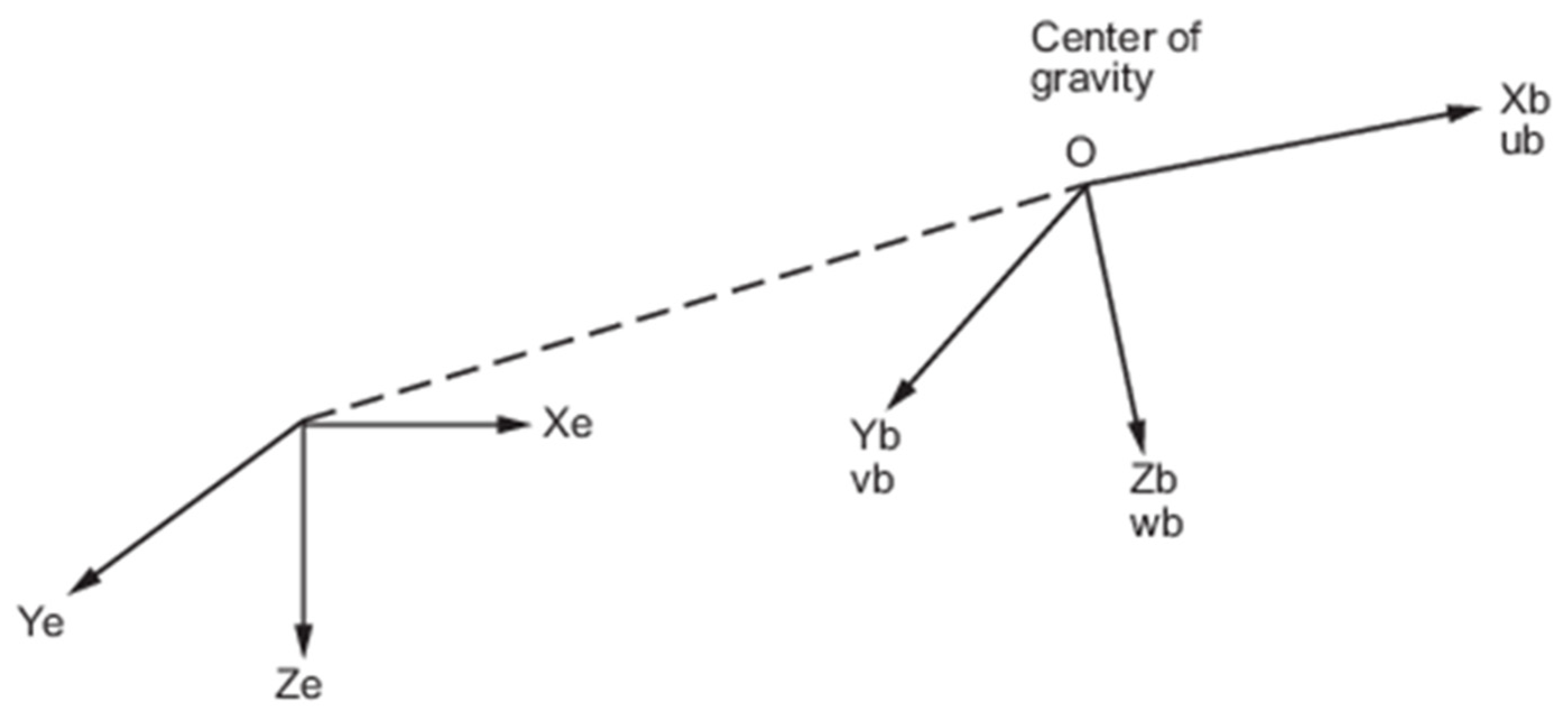
2.1. Simulink Model

The trajectory of the rocket was computed using a model based on Matlab–Simulink R2023B^©. This model computes the behavior of a solid rocket engine based on input physical characteristics and propellant types. Key assumptions within the model include the following:

• The atmosphere was modelled using the International Standard Atmosphere (ISA) model [25].
• The assumed rockets are non-spinning and stabilized with fixed wings.
• The flat earth reference frame is assumed to be inertial, which is acceptable for low-range rockets.
• Gravity is considered constant throughout the flight.
• The rocket operates under subsonic conditions, according to numerically and experimentally simulated design data.
• High-order aerodynamic effects, arising from unsteady aerodynamics, are considered negligible. While these reduce accuracy, particularly under conditions of high maneuvering angles, the resulting error from this assumption remains comparable in magnitude to other errors associated with other modeling assumptions and adopted simplifications.
• Erosive burning effects were not considered.
• The rocket was modelled as a rigid body.

The model employs two reference frames, as depicted in Figure 2. The flat earth reference frame (marked as e) is treated as inertial, allowing for the omission of forces arising from the earth’s motion relative to fixed stars. This reference frame is defined as the z-axis being aligned vertically, which is consistent with the direction of gravitational acceleration.

The body-fixed reference frame (marked as b) is anchored at the rocket’s center of gravity (COG), with the x-axis being aligned along the missile’s principal longitudinal axis, while the y- and z-axes are perpendicular to it, forming a right-handed (dextrorse) coordinate system.

Conversion between these frames is facilitated through the use of quaternions. Figure 3 depicts a principal view of the model.

The core of the model is encapsulated within an integration block that employs a 6DoF [26] variable mass block in Simulink to integrate state variables. The initial conditions are specified in terms of the initial velocity, position, zenith, and azimuth angles of the ramp. The model also incorporates a control mechanism designed to terminate the simulation upon reaching apogee, which is identified by a threshold in vertical velocity and signs of changes in the altitude rate. The state output from the integration block is further refined by five distinct blocks to produce the integrated state.

The atmosphere block calculates air state variables utilizing the International Standard Atmosphere (ISA) model and incorporates the Von Karman Wind Turbulence Model [27].

The aerodynamic block calculates aerodynamic coefficients using curve-fitting techniques on simulation data of Computational Fluid Dynamics (CFDs). It takes into account variations in the angle of attack and Mach number. Aerodynamic forces and moment coefficients, expressed in the reference frame of the body axes as a function of the angle of attack (AOA °deg), are provided in Appendix A.

The engine block models the behavior of the solid rocket engine based on experimentally driven parameters from static tests, providing outputs such as the remaining propellant mass, the mass flux from the nozzle, and the thrust magnitude.

The structure block calculates the rocket’s rigid body properties, including the inertia tensor (considering the parallel axis theorem in tensor formulation), its rate-of-change time, the center of gravity, and mass. The assumption that the rocket behaves as a rigid body eliminates the need to consider internal forces, resulting in a simplified, lumped model.

The forces and torque block aggregate the effects of all preceding blocks, adding additional effects and constraints. These include the consideration of aerodynamic damping, the impact of maneuvers on the thrust vector, and constraints imposed by the launch ramp. The total set of forces and torques is calculated with respect to the body axis.

The Ordinary Differential Equations (ODEs) employed in this study are solved using the ode23 stiff solver with Modified Rosenbrock method. This choice was motivated by the coexistence of slow and fast dynamics within this system.

2.2. Optimization Script

A genetic algorithm (GA) [28] was selected, among other optimization tools, for this task due to the problem’s complexity and for its capability to avoid local minima solutions.

The optimization problem was framed as the minimization of a cost function, which involves two distinct design variables, the zenith ramp angle and thrust deflection angle. To streamline the problem, a further assumption is introduced: the absence of constant wind, which permits the treatment of motion as predominantly two-dimensional within the X–Z plane. This simplification constrains maneuvers to the longitudinal plane, requiring the target to also reside within it. Although this assumption reduces one degree of freedom, it does not significantly impair maneuverability; the lost degree can be compensated by adjusting the rocket’s azimuth. Under these conditions, the cost function is articulated as the minimum Euclidean distance between the trajectory and the target, with [x, z] representing an n²-dimensional vector of the trajectory points, where n denotes the number of integration steps, and (x_t, z_t) represent the target coordinates. The cost function is defined as follows:

$$Cost function=min\left(\sqrt{{\left(x-x_t\right)}^2+{\left(z-z_t\right)}^2}\right)$$

The design variables chosen are as follows:

• The ramp zenith: This is defined as the angle between the earth’s vertical-to-surface axis and the ramp axis. This integer variable can adopt discrete values equal to 0°, 15°, 30°, or 45° sexagesimal degrees, representing a classified discrete ramp movement’s range.
• The thrust deflection angle: this represents the output of the thrust vector and is treated as a continuous variable bounded between 0° and 5°.

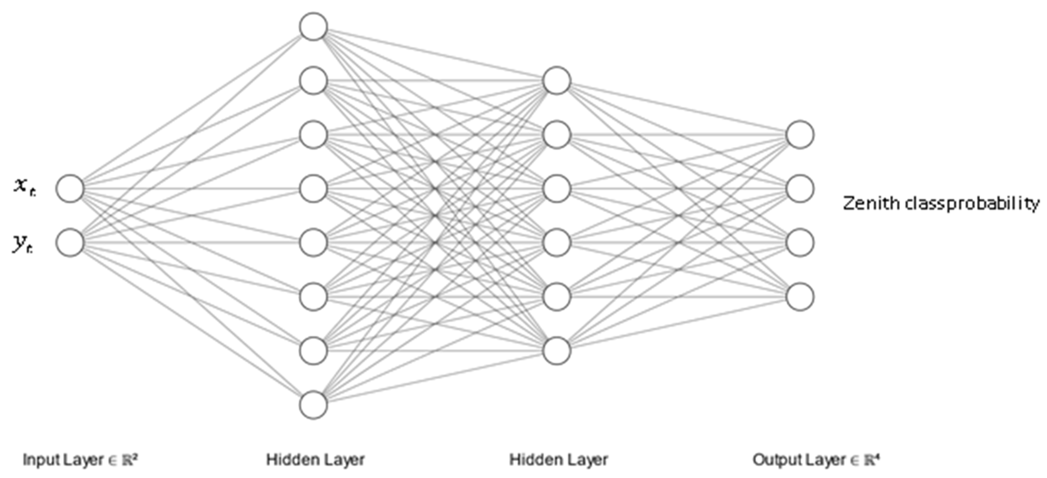
The settings for the GA optimization algorithm are specified in

Table 1. Settings for GA optimizer.

Description	Value
Population size	50
Maximum number of generations	200
Constraint tolerance	1 × 10−3
Creation function rate	0.8
Crossover function	Arithmetic crossover
Mutation function	Adaptive feasible mutation
Selection function	Roulette wheel selection
Distance measurement function	Crowding distance
Nonlinear constraint algorithm	Augmented Lagrangian
Elite count	2
Fitness limit	1
Fitness scaling function	Rank scaling
Function tolerance	1 × 10−6

.

After optimization, the results are post-processed to compile a comprehensive matrix of outcomes.

2.3. Neural Network

The problem was conceptualized, as before, with two inputs, representing the spatial coordinates of the target, and two outputs, denoting the two design variables (the azimuth and maneuvering angles). The surrogated model is trained using result matrices obtained from the genetic algorithm (GA) previously described.

Considering the integer constraint on the zenith angle, the optimization procedure is structured into two phases to procure the optimum solution:

• Classification Algorithm: initially, the solution space is partitioned through a classification strategy, with the zenith angle serving as the clustering criterion.
• Regression: following the classification stage, a regression is adopted to forecast the continuous deflection angle based on the target coordinates, tailoring, for each cluster, the maneuverer’s deflection angle.

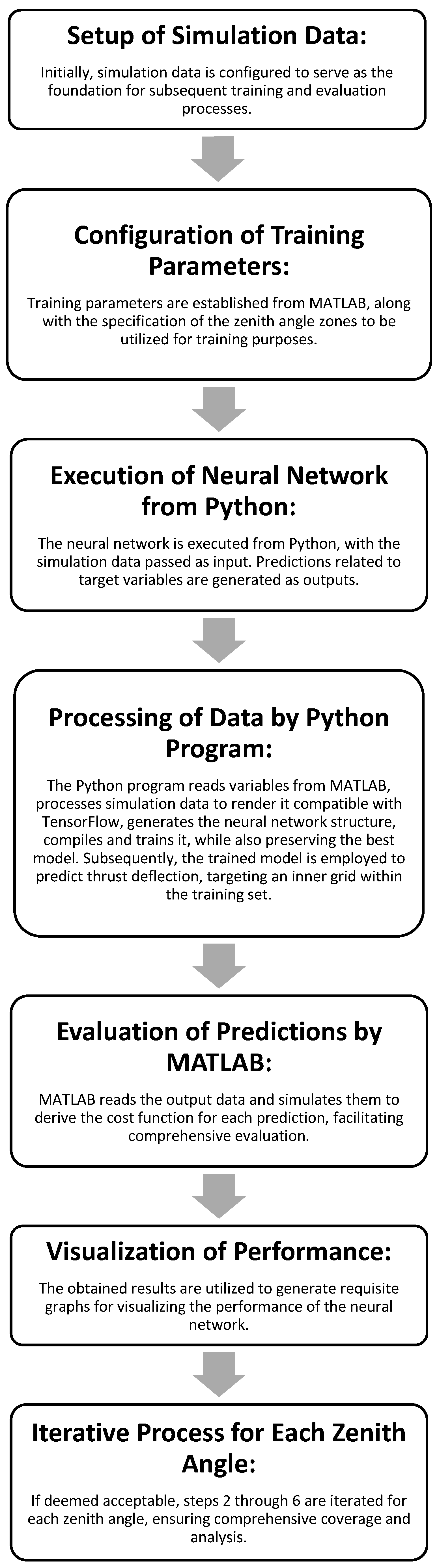
The utilization of this cascade strategy facilitates effective navigation through the integer constraints of the problem, ensuring accurate predictions of both the zenith and deflection angles.

The neural networks were developed employing TensorFlow [29], and integration with Matlab is achieved through a dedicated Python script which automates testing and data post-processing for performance evaluation.

For the classification neural network, the parameters are reported in

Table 2. Settings for classification neural network.

Description	Value
Loss function	Categorical Crossentropy
Accuracy metric	Accuracy
Batch size	512
Hidden layers	10, with a predetermined neuron distribution
Activation function	ReLU for hidden layers and Softmax for the output layer
Number of epochs	10,000

, while those for Regression NN are reported in

Table 3. Settings for classification neural network.

Description	Value
Loss function	Mean Square Error
Accuracy metric	Mean Absolute Error
Batch size	512
Hidden layers	10, with a specific distribution of neurons per layer
Activation function	ReLU for hidden layers and linear for the output layer
Number of epochs	10,000

. A schematic representation of the implemented NN is shown in Figure 4 (classification problem) and Figure 5 (regression problem):

Moreover, a callback function is employed to retain the optimal model during training, and a scaler is applied for data normalization, using the Scikit-learn library [30], ensuring consistent performance and straightforward integration with other systems.

2.4. Workflow

The steps of the implemented workflow are summarized in Figure 6a and Figure 7, while Figure 6b depicts the target point evaluated for the genetic algorithm. The selected target points were established based on the achievable range of the engine, as determined through prior experimental analyses.

A generic contour outcome of the deflection angle obtained by the GA is shown in Figure 6c.

3. Results

This section provides the outcomes obtained during the simulation campaign. The key metrics gleaned from the simulations encompass the following:

• The time elapsed until the target is reached.
• The zenith angle of the launch ramp.
• The deflection angle of the thrust required for implementing maneuvers.
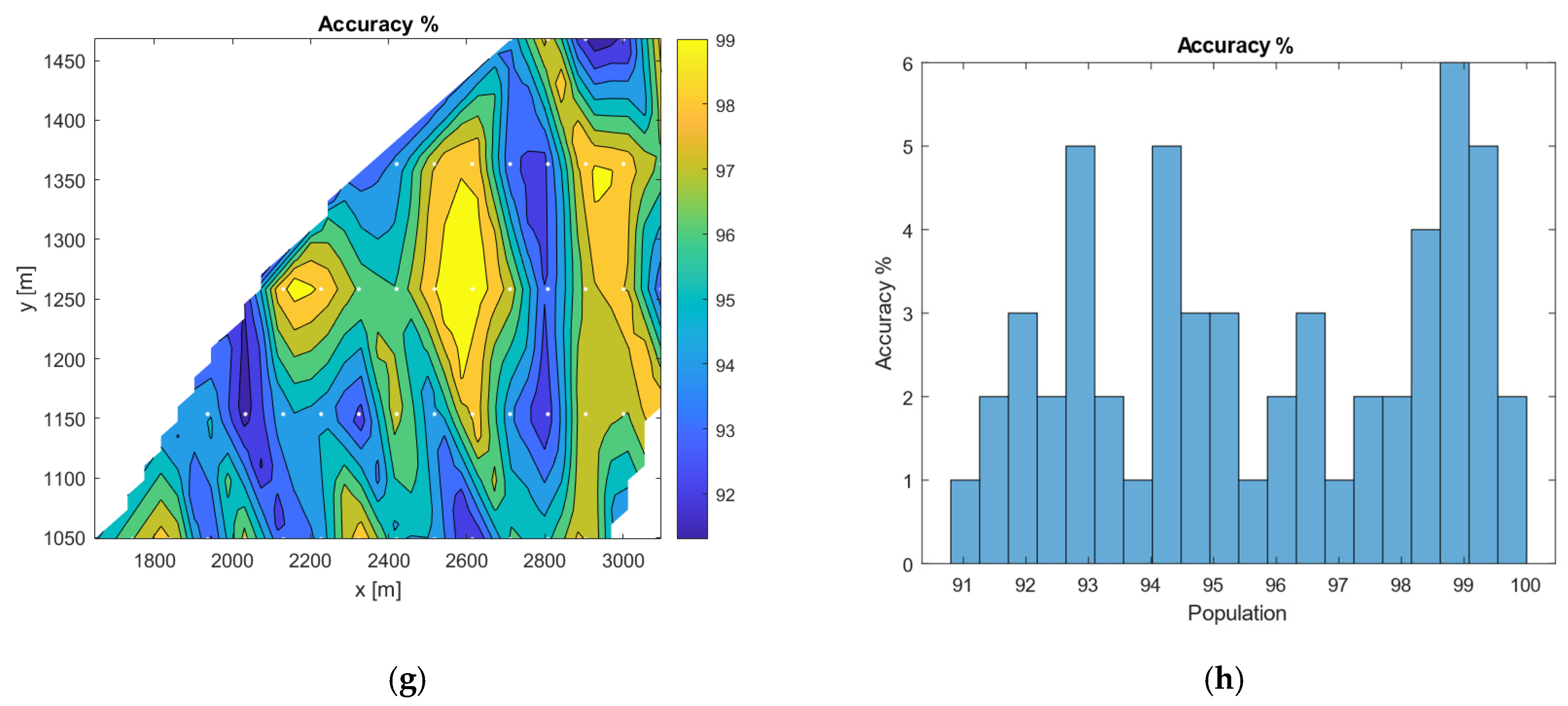
• Accuracy, quantified as a percentage, where 100% signifies exact alignment with the target’s center of gravity, and 0% indicates a failure to meet the target.

These data are depicted through contour plots and histograms.

3.1. GA Results

The results shown in Figure 8 offer a comprehensive overview of the outcomes achieved through the genetic algorithm (GA).

The time contour plot depicted in Figure 8a confirms the initial hypothesis, illustrating that the pursuit of distant targets necessitates longer flight times.

A detailed inspection of the zenith deflection, illustrated in the graphs in Figure 8b, uncovers four distinct zones, which correspond to the zenith angle’s four-class constraint; within these zones, transitional areas are distinctly visible. Furthermore, the behavior within each subzone begins with high maneuvers angles (Figure 8c) and narrows down to a minimum, suggesting a consistent inner pattern that corroborates the findings shown in the zenith contour plot.

The error metrics, expressed in Figure 8c as a percentage of the total distance, generally hover near zero, with exceptions in regions characterized by the maximum distance and minimum height, where reaching these boundary areas presents trajectory challenges. This observation aligns with the accuracy histogram, Figure 8d, which demonstrates that nearly all optimized test cases achieve their targets with minimal error, which is consistent with the expectations set by the error contour plot. Notably, instances of reduced accuracy are predominantly found in boundary zones.

The depiction in Figure 8f of a central trajectory enriches our comprehension of the launch phases: it starts with the initial position of the ramp, highlighted in green; followed by a variable maneuver phase, in red; and concludes with a ballistic trajectory, in blue.

The minimal occurrence of low-accuracy cases, as depicted in Figure 8e, suggests that excluding such targets and narrowing the domain does not markedly detract from the overall utility of this approach. A subsequent analysis, which excluded targets deemed unachievable, revealed that the algorithm maintains a high level of performance, with accuracy rates ranging between 91% and 99% across all simulations. The overall amended results are shown in Figure 9, with the same exposition logic of Figure 8.

3.2. Classification

The neural network results are reported in Figure 10. For a comprehensive assessment of the neural network’s capabilities, a comparative analysis with the results obtained from the genetic algorithm (GA) was conducted, focusing on the discrete zenith angle of the ramp. This comparison, whose results are depicted through contour plots in Figure 10a,b, provides preliminary positive insights about the overall agreement level between GAs and the classification method. A further observation of the network’s proficiency is evidenced by a minimum training loss of 2.38 × 10⁻⁹, as shown in Figure 10c, indicating a highly favorable outcome.

Lastly, Figure 10d introduces the confusion matrix; notably, an analysis of the latter revealed an impressive accuracy rate of 100%, with no confusion cases reported.

3.3. Regression

An evaluation of the regression neural network for thrust deflection was conducted using the genetic algorithm (GA) method. The table below (

Table 4. NN loss performance.

Zenith Angle [°]	Minimum Loss
0°	1.3869 × 10−6
15°	3.0502 × 10−6
30°	5.4031 × 10−6
45°	1.8426 × 10−8

) presents the minimum loss for each model, calibrated for specific zenith angle zones and calculated using the Mean Square Error (MSE) function (Table 3). The MSE serves as an effective estimator, as it represents the mean of the squared Euclidean distances. This approach allows for the correlation of the loss function with a meaningful physical interpretation, highlighting its ability to directly quantify prediction accuracies. Observing Table 4, it is evident that the training results are satisfactory, demonstrating the effectiveness of these models.

A detailed examination of the results can be conducted through the observation of model accuracies, depicted via histograms and contours, akin to prior analyses. From Figure 11, it is clear that the models generally perform as expected, with a marked decrease in accuracy being observed near the edges of the domain. However, it is noteworthy that the model corresponding to the 45-degree configuration (Figure 11c) exhibits consistently high accuracy values across the entire domain.

3.4. Testing the Neural Network on a New Batch

A final test was conducted on a new batch of target points, distinct from those initially considered yet still within the operational range of the missile system. These new points were obtained from the interpolated midpoint of those calculated for the GA reported in Figure 6b. From the results shown in Figure 12, several key observations can be made. First, the structure of the solutions generated for this new batch closely mirrors those derived from the GA, affirming the algorithm’s robustness and adaptability even in the test set. However, as anticipated, a slight degradation in accuracy towards the domain’s boundaries was observed, particularly highlighted in Figure 12d,f.

This issue is largely due to the lower density of data points in these regions. A potential solution involves implementing an adaptive training set, which would update the initial dataset by increasing the number of points specifically in areas requiring a genetic algorithm (GA) solution. Despite this, the overall performance remains commendably high. Approximately 86% of the instances were found to achieve an accuracy rate exceeding 80%.

3.5. Computational Cost Comparison

The results of a focused comparative analysis on specific target coordinates (149 m, 1101 m) are reported in

Table 5. Results of a comparison between GA and NN with target points (x 149 m, y 1101 m), (CPU: Intel Core i7-11,700 K, 8 core/8 thread, 3.6 GHz base, 4.9 GHz boost. RAM: 32 GB DDR4, 3200 MHz GPUNVIDIA GeForce RTX 1660 6 GB. Python: 3.8.5. TensorFlow: 2.4.0).

	Thrust Deflection [deg]	Zenith [deg]	Accuracy [%]	Elapsed Time [s]
GA	2.35	0	95%	58.98
NN	2.29	0	89%	1.05
COMPARATION	2.55%	0%	−6.32%	98.22%

. The reported data elucidate the trade-offs involved in machine learning (ML) techniques, revealing a nuanced balance between accuracy and efficiency. Although a marginal decrement in accuracy is observed following the adoption of ML strategies, the data notably underscore a substantial reduction in the elapsed time for the computations.

4. Conclusions

In conclusion, this paper introduces a hybrid methodology that represents a significant advancement in the optimization of solid rocket missile trajectories. By combining machine learning (ML) with genetic algorithms (GAs), this approach has proven effectiveness in optimizing missile trajectories with high accuracy. Additionally, ML integration streamlines real-time trajectory predictions and optimization, reducing time and resource consumption. The promising, yet preliminary, results of this methodology suggest that this simple approach can be employed to develop more complex control methods in the future.

References

1. Belkin, P.; Ek, C.; Mages, L.; Mix, D.E. NATO’S 60th Anniversary Summit. In European Economic and Political Developments; NATO: Washington, DC, USA, 2009; Available online: https://apps.dtic.mil/sti/pdfs/ADA496595.pdf (accessed on 1 November 2024).
2. Chaurasiya, P.; Sawardekar, S.; Rautela, R. Enhancing Air and Missile Defense System with IoT Solution: A Conceptual Approach. Int. J. Res. Appl. Sci. Eng. Technol. 2023, 11, 1200–1207. [Google Scholar] [CrossRef]
3. Dvorkin, V. Impact of missile defense systems on strategic stability and prospects for nuclear disarmament. World Econ. Int. Relat. 2019, 63, 5–12. [Google Scholar] [CrossRef]
4. Klimov, V. The Missile Defense systems and concepts of limited nuclear war. World Econ. Int. Relat. 2022, 66, 16–24. [Google Scholar] [CrossRef]
5. Khalil, M.; Ahmed, M.Y.M. Flight Performance and Dispersion Analysis for a Flexible Tactical Missile. J. Spacecr. Rocket. 2023, 60, 1297–1307. [Google Scholar] [CrossRef]
6. Sahoo, S.; Dalei, R.K.; Rath, S.K.; Sahu, U.K. Selection of PSO parameters based on Taguchi design-ANOVA-ANN methodology for missile gliding trajectory optimization. Cogn. Robot. 2023, 3, 158–172. [Google Scholar] [CrossRef]
7. Cai, Z. Missile trajectory defense planning and data simulation based on deep learning algorithm. Soft Comput. 2023, 1, 1–10. [Google Scholar] [CrossRef]
8. Benton, N. The role of Russian air and missile defense systems. Comp. Strat. 2022, 47, 483–497. [Google Scholar] [CrossRef]
9. Haggard, S.; Cheung, T.M. North Korea’s nuclear and missile programs: Foreign absorption and domestic innovation. J. Strat. Stud. 2021, 44, 802–829. [Google Scholar] [CrossRef]
10. Khan, F.H. Strategic Risk Management in Southern Asia. J. Peace Nucl. Disarm. 2022, 5, 369–393. [Google Scholar] [CrossRef]
11. Yingbo, H.; Yong, Q. THAAD-Like High Altitude Theater Missile Defense: Strategic Defense Capability and Certain Countermeasures Analysis. Sci. Glob. Secur. 2003, 11, 151–202. [Google Scholar] [CrossRef]
12. Hussain, M.Z.; Ahmed, R.Q. Space Programs of India and Pakistan: Military and Strategic Installations in Outer Space and Precarious Regional Strategic Stability. Space Policy 2019, 47, 63–75. [Google Scholar] [CrossRef]
13. Pirsalami, F.A.; Shirzadi, E. Regional deterrence, strategic challenges, and Saudi Arabia’s missile development program. Dig. Middle East Stud. 2023, 32, 281–299. [Google Scholar] [CrossRef]
14. Zhang, L.; Gong, C.; Su, H.; Andrea, D.R. Design Methodology of a Mini-Missile Considering Flight Performance and Guidance Precision. J. Syst. Eng. Electron. 2024, 35, 195–210. [Google Scholar] [CrossRef]
15. Li, J.; Jing, Z.; Zhang, X.; Zhang, J.; Li, J.; Gao, S.; Zheng, T. Optimization design method of a new stabilized platform based on missile-borne semi-strap-down inertial navigation system. Sensors 2018, 18, 4412. [Google Scholar] [CrossRef] [PubMed]
16. Wang, Y.; Lei, H.; Ye, J.; Bu, X. Backstepping sliding mode control for radar seeker servo system considering guidance and control system. Sensors 2018, 18, 2927. [Google Scholar] [CrossRef]
17. Tuncer, O.; Cirpan, H.A. Adaptive fuzzy based threat evaluation method for air and missile defense systems. Inf. Sci. 2023, 643, 119191. [Google Scholar] [CrossRef]
18. Multi-agent decision support system for missile defense based on improved PSO algorithm. J. Syst. Eng. Electron. 2017, 28, 514–525. [CrossRef]
19. Das, A.K.; Acharyya, K.; Mankodi, T.K.; Saha, U.K. Fluidic Thrust Vector Control of Aerospace Vehicles: State-of-the-Art Review and Future Prospects. J. Fluids Eng. 2023, 145, 080801. [Google Scholar] [CrossRef]
20. Afridi, S.; Khan, T.A.; Shah, S.I.A.; Shams, T.A.; Mohiuddin, K.; Kukulka, D.J. Techniques of Fluidic Thrust Vectoring in Jet Engine Nozzles: A Review. Energies 2023, 16, 5721. [Google Scholar] [CrossRef]
21. Kim, K.U.; Kang, S.; Kim, H.J.; Lee, C.-H.; Tahk, M.-J. Realtime agile-turn guidance and control for an air-to-air missile. In Proceedings of the AIAA Guidance, Navigation, and Control Conference, Toronto, ON, Canada, 2–5 August 2010. [Google Scholar] [CrossRef]
22. Jung, C.-G.; Kim, B.; Jung, K.-W.; Lee, C.-H. Thrust Integrated Trajectory Optimization for Multipulse Rocket Missiles Using Convex Programming. J. Spacecr. Rocket. 2023, 60, 957–971. [Google Scholar] [CrossRef]
23. Biberstein, J.X.; Tal, E.; Karaman, S. Thrust Vectoring of Small-scale Solid Rocket Motors Using Additively Manufactured Jet Vanes. In Proceedings of the AIAA Propulsion and Energy 2021 Forum, Virtual, 9–11 August 2021. [Google Scholar]
24. The MathWorks—MATLAB & SIMULINK. IEEE Circuits Syst. Mag. 2008, 6, 77. [CrossRef]
25. Young, T.M. International Standard Atmosphere (ISA) Table. In Performance of the Jet Transport Airplane: Analysis Methods, Flight Operations and Regulations; Wiley: Hoboken, NJ, USA, 2017. [Google Scholar] [CrossRef]
26. Mikhailov, V.G. Data transmission with Simulink on 6-DoF platform on CAN BUS. System Anal. Appl. Inf. Sci. 2021, 1, 29–37. [Google Scholar] [CrossRef]
27. Hajjem, M.; Victor, S.; Melchior, P.; Lanusse, P.; Thomas, L. Wind turbulence modeling for real-time simulation. Fract. Calc. Appl. Anal. 2023, 26, 1632–1662. [Google Scholar] [CrossRef]
28. Oluleye, B.; Leisa, A.; Leng, J.; Dean, D. A Genetic Algorithm-Based Feature Selection. Int. J. Electron. Commun. Comput. Eng. 2014, 5, 899–905. [Google Scholar]
29. Abadi, M.; Barham, P.; Chen, J.; Chen, Z.; Davis, A.; Dean, J.; Devin, M.; Ghemawat, S.; Irving, G.; Isard, M.; et al. TensorFlow: A system for large-scale machine learning. In Proceedings of the 12th USENIX Symposium on Operating Systems Design and Implementation, Savannah, GA, USA, 2–4 November 2016. [Google Scholar]
30. Gevorkyan, M.N.; Demidova, A.V.; Demidova, T.S.; Sobolev, A.A. Review and comparative analysis of machine learning libraries for machine learning. Discret. Contin. Model. Appl. Comput. Sci. 2019, 27, 305–315. [Google Scholar] [CrossRef]
Figure 1. Patented section view of small rocket with integrated cooling and thrust vectoring.
Aerospace 11 00912 g001
Figure 2. Reference frames.
Aerospace 11 00912 g002
Figure 3. Model overview.
Aerospace 11 00912 g003
Figure 4. A schematic of the classification NN.
Aerospace 11 00912 g004
Figure 5. A schematic of the regression NN.
Aerospace 11 00912 g005
Figure 6. Optimal trajectory calculation: (a) workflow diagram, (b) target grid, (c) post-processing graph.
Aerospace 11 00912 g006
Figure 7. NN training and extraction of the model.
Aerospace 11 00912 g007
Figure 8. GA optimization algorithm: (a) time contour plot, (b) zenith contour plot, (c) maneuver angle contour plot, (d) accuracy contour plot, (e) accuracy histogram, (f) typical trajectory.
Aerospace 11 00912 g008aAerospace 11 00912 g008b
Figure 9. GA optimization algorithm with restricted domain: (a) time contour plot, (b) zenith contour plot, (c) maneuver angle contour plot, (d) accuracy contour plot, (e) accuracy histogram, (f) typical trajectory.
Aerospace 11 00912 g009aAerospace 11 00912 g009b
Figure 10. Performance of NN classification algorithm: (a) neural network zenith angle; (b) GA zenith angle. (c) the network’s proficiency; (d) the confusion matrix.
Aerospace 11 00912 g010
Figure 11. Performance of NN classification algorithm under the different zenith angles: (a,b) 0°, (c,d) 15°, (e,f) 30°, and (g,h) 45°.
Aerospace 11 00912 g011aAerospace 11 00912 g011b
Figure 12. Different batch performance evaluations with NN: (a) time contour plot, (b) zenith contour plot, (c) maneuver angle contour plot, (d) accuracy contour plot, (e) accuracy histogram, (f) typical trajectory.
Aerospace 11 00912 g012aAerospace 11 00912 g012b