Real-Time LiDAR–Inertial Simultaneous Localization and Mesh Reconstruction

Abstract

In this paper, a novel LiDAR–inertial-based Simultaneous Localization and Mesh Reconstruction (LI-SLAMesh) system is proposed, which can achieve fast and robust pose tracking and online mesh reconstruction in an outdoor environment. The LI-SLAMesh system consists of two components, including LiDAR–inertial odometry and a Truncated Signed Distance Field (TSDF) free online reconstruction module. Firstly, to reduce the odometry drift errors we use scan-to-map matching, and inter-frame inertial information is used to generate prior relative pose estimation for later LiDAR-dominated optimization. Then, based on the motivation that the unevenly distributed residual terms tend to degrade the nonlinear optimizer, a novel residual density-driven Gauss–Newton method is proposed to obtain the optimal pose estimation. Secondly, to achieve fast and accurate 3D reconstruction, compared with TSDF-based mapping mechanism, a more compact map representation is proposed, which only maintains the occupied voxels and computes the vertices’ SDF values of each occupied voxels using an iterative Implicit Moving Least Squares (IMLS) algorithm. Then, marching cube is performed on the voxels and a dense mesh map is generated online. Extensive experiments are conducted on public datasets. The experimental results demonstrate that our method can achieve significant localization and online reconstruction performance improvements. The source code will be made public for the benefit of the robotic community.

1. Introduction

Simultaneous Localization and Mapping (SLAM) systems are fundamental technologies of intelligent vehicles. Though the basic function of SLAM [1] is to estimate trajectory accurately in unknown environment, high-quality dense mapping results not only benefit the localization performance, but also are necessary for high-level human-given tasks [2]. Thus, in recent years, 3D dense mapping has drawn much research attention. In this paper, we focus on real-time 3D dense mapping, which means that we have to rely on odometry results to aggregate map points and generate an accurate mesh model efficiently.

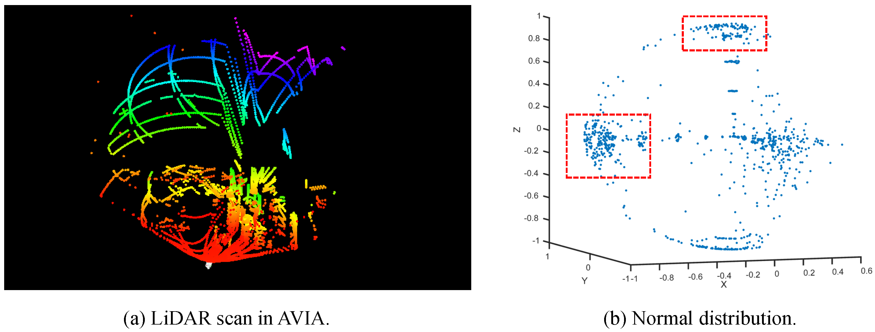
In terms of odometry, there are still inherent errors that are less studied in the existing LiDAR–inertial odometry methods. In recently years, LiDAR–inertial odometry has demonstrated its superior performance to odometry based on other sensor configurations. FastLIO2 [3] is the most typical and widely used LiDAR–inertial odometry method. Many novel odometry methods have been proposed based on the FastLIO2 framework. However, there remain two issues. Firstly, during the LiDAR scanning process, the inertial measurement units (IMUs) are incrementally integrated and then provide prior pose estimation for later LiDAR scan alignment. Essentially, the IMU is used to avoid LiDAR scan matching degeneration, especially in extreme environments. Odometry precision is mostly determined by the LiDAR scan-matching part. IMU-based prior constraints, scan-to-map matching, and point-to-plane registration are the three key factors for the success of FastLIO2. However, to further promote odometry precision, it is expected that the LiDAR measurements can provide rigid and enough pose estimation optimization, which requires that the LiDAR points’ corresponding residuals are spatially distributed evenly. However, such a requirement cannot be well satisfied. In most environments, the LiDAR measuremens are generally redundant in some directions, such as the ground, and are sparse in the other directions. Once the redundant observations play dominant roles during the optimization process, the optimal state estimation tends to overfit the redundant observations and thus depart from the real true state, which means that odometry precision is degraded.

Odometry is an essentially nonlinear optimization problem. Its cost function is highly nonlinear and the linearization error is unavoidable. The Kalman Filter (KF) and its variants are widely used in LiDAR–inertial odometry. However, they are constructed based on the Gaussian distribution hypothesis and aim to maximize the fused distribution of prior and posterior Gaussian distributions. Once the Gaussian distribution hypothesis is not well satisfied, the filter performance is thus degraded. The Gauss–Newton (GN) algorithm is another effective alternative for solving the nonlinear optimization problem. Though linearization errors are also unavoidable in GN, it computes the optimal iterative state based on second-order approximation, which is more robust to the Gaussian distribution approximation error. Thus, in this paper, we stress the importance of the GN algorithm in LiDAR–inertial odometry.

In terms of dense mapping, a common solution is to construct a TSDF-based implicit surface representation model [4] and then use the marching cube algorithm [5] to represent the surface explicitly by a set of triangle faces. For each voxel, its SDF value is defined as its nearest distance from its center points to its surface along LiDAR rays. These faces are targeted to approximate the zero-SDF-value surface. Marching cube is a well-developed algorithm; thus, the bottlenecks of dense mapping are determined by the TSDF voxel maintaining efficiency and the SDF values computing accuracy. In the existing TSDF-based mapping methods [6,7,8,9], the full 3D space is voxelized and the scale of the TSDF voxels is significantly increased with the environmental size. Since the marching cube algorithm is required to traverse all the voxels, the computational efficiency is limited in a large-scale environment. Furthermore, the SDF values are generally computed based on ray-casting mechanism, which is achieved by averaging the voxel-to-LiDAR-beam-end distances. However, given the 3D LiDAR measurements are noisy and sparse, such a mechanism is prone to errors and the surface normal information is not involved. Though a gradient field is then introduced in VoxField [10] and significantly benefits the mapping accuracy, the computational burden is also enlarged due to gradient field maintenance and fails to meet the online requirement. Also, its gradient field is also sensitive to LiDAR points’ sparsity.

An effective way to alleviate the efficiency issue of dense mapping is to avoid processing all the voxels and focus on the voxels that are occupied. Recently, SLAMesh [11] was proposed and it can achieve real-time dense mapping, which is most related to ours. In each occupied voxel, the authors project the points to the three coordinate directions, respectively, and approximate the surface by estimating the surface function using a Gaussian Process [12,13,14]. Since they firstly sample vertices evenly on the estimated surface, triangle faces can be directly generated by connecting neighbor vertices. Then, the global mesh model is obtained by accumulating the faces. Though they significantly improve the mapping efficiency, a densely performing Gaussian Process still increases the computational cost. One important feature of SLAMesh is that the faces are generated separately in each voxel. This means that faces between neighboring voxels tend to fail to meet the smoothness requirement. Furthermore, their Gaussian Process-based surface approximation is implemented in the full voxel space. However, such a configuration tends to generate redundant surface estimation when the voxel is not fully occupied.

The marching cube algorithm has the advantage of generating a smooth, accurate, and less redundant dense surface. It is also efficient due to the application of a look-up table. Thus, in this paper, we propose a novel dense mapping system that fuses the advantages of TSDF-based mapping and the SLAMesh-like mapping paradigm. Specifically, firstly, we only perform voxelization in the occupied space and implement a voxel insert, retrieval, and update mechanism based on $std::unordered\_map$ in C++. Then, for each voxel, we compute and update the SDF value of its center point by IMLS surface representation only using the contained map points, which can avoid estimating explicit surface function and can directly use the LiDAR points and normals to compute the voxel-to-surface distance accurately. Thirdly, we traverse all the updated voxels, and for each voxel, we formulate a cube according to its neighboring voxels. The marching cube algorithm is then performed on the cube to generate vertices and faces.

The main contributions of this paper are summarized as follows.

• A residual-density-driven Gauss–Newton algorithm is proposed and applied in LiDAR–inertial odometry, which can promote pose estimation accuracy.
• A novel TSDF-free dense mapping paradigm is proposed, which is more flexible and scalable than the traditional TSDF mapping paradigm. IMLS surface representation is introduced to compute SDF values accurately and efficiently, which is superior to the ray-casting-based mechanism.
• We will release our code to benefit the robotics community.

The rest of this paper is organized as follows. Section 2 presents the related work. Section 3 gives the notations and Section 4 presents the details of the proposed method. The experimental evaluations are shown in Section 5. Section 6 concludes the paper.

2. Related Work

LiDAR–inertial odometry: The first kinds of methods achieving LiDAR–inertial odometry are based on factor graphs. Such methods include LIOSAM [15], LiLi-OM [16], and FF-LINS [17]. These methods incorporate feature-based LiDAR scan constraints and IMU pre-integration constraints into local and global pose graphs. Feature extraction, keyframe selection, sliding windows, and various marginalization mechanisms are then proposed in these methods to achieve better performance. Though factor graph-based methods are flexible and powerful, they are also known efficiency issues, especially when the factor scale grows. The second kinds of methods are based on filters. Such methods include FastLIO2 [3], FasterLIO [18], iG-LIO [19], LOG-LIO [20], PointLIO [21], and Direct-LIO [22]. FastLIO2 proposed IESKF-based scan-to-map registration and an efficient map data structure, i-kdtree. FastLIO2 has drawn much research attention due to its accuracy and efficiency performance. FasterLIO further promotes efficiency by using incremental voxels (iVox) as a point cloud spatial data structure. iVox is a novel 3D voxel data structure supporting incremental insertion and parallel approximated k-NN queries. Instead of implementing raw point-to-map registration, iG-LIO introduces the GICP [23] registration algorithm into LiDAR–inertial odometry to achieve more robust and accurate LiDAR constraint computation. Among these methods, one common module is LiDAR scan undistortion using IMU measurements. Considering that such a process exhibits errors, PointLIO and Direct-LIO proposed a novel point-by-point LIO framework, which updates the state at each LiDAR point measurement. This framework allows an extremely high-frequency odometry output and fundamentally removes the artificial in-frame motion distortion [21]. Furthermore, Wang et al. proposed a hierarchical LIO, which is composed of low-level LiDAR–inertial odometry based on the IEKF and high-level factor graph optimization [24]. The third kind of method is incorporating LiDAR–inertial odometry into the mapping process. In SLICT [25], the mapping thread maintains an octree-based global map of multi-scale surfels that can be updated incrementally. The odometry thread performs point-to-surfel registration. In LIO-GVM [26], the authors argue that directly registering the source points to the nearest target points would generate mismatches and generating a map by directly aggregating LiDAR points is not elegant. They extend and apply VGICP [27] in LiDAR–inertial odometry and probabilistic voxel-based map maintenance. From these methods, we can see that developing a more adaptable map data structure instead of a simple point set and incorporating novel representation into LiDAR–inertial odometry can effectively promote the system performance. Among these methods, researchers focus on alleviating the odometry degeneration by developing the odometry itself. However, there exists inherent degeneration in some environments due to the LiDAR scanning mechanism. The LiDAR sensors tend to hit more points on the ground and fewer points are hit on informative areas. Redundant and less-informative points tend to degrade any LiDAR odometry.

Dense mapping methods: KinectFusion [28] is the first method that achieves visual-based real-time 3D reconstruction using TSDF-based environmental representation. Since it was proposed in KinectFusion, the basic TSDF-based mapping framework has been widely confirmed in the literature, which consists of TSDF-based representation, ray-casting-based TSDF updating, and marching cube-based mesh model generation. The main challenge turns out to be how to maintain the TSDF map. Then, lots of variations of KinectFusion have been proposed to alleviate the problem. BundleFusion [29] pays more attention to global camera pose alignment and optimization. The authors directly integrate the observations into the TSDF-based map. To maintain the integration accuracy, they reintegrate the observations after the global poses are updated. Notice that the drift error is hard to tackle during the TSDF mapping process, since the map should be immediately updated once the poses are corrected; C-blox [7] is proposed and it formulates the global map as a set of submaps and maintains the relative pose between submaps. TSDF mapping efficiency is also another important issue. In Vox-blox [6], because the ray-casting operation in a 3D environment is time-cosuming, the TSDF updating performance is effectively prompted by the proposed grouped ray casting mechanism. To further improve the mapping efficiency, VDB-Fusion [9] introduces an OpenVDB data structure [30] to build a TSDF map. With the help of OpenVDB, the TSDF voxels are more efficient when extended, updated, and retrieved. Notice that the ray-casting-based TSDF value computing accuracy is limited. Lius et al. [31] propose a novel surface normal estimation based on Gaussian confidence. Their SDF values are accurately computed by point-to-surface distance. However, their method cannot be applied in an incremental strategy. To alleviate such a problem, Vox-Field [10] constructs and incrementally updates gradient voxels. Each TSDF value is updated considering the normal cues provided by the corresponding gradient voxels.

Recently, a novel dense mapping paradigm was proposed by the creators of SLAMesh [11]. Instead of approximating the surface by TSDF voxels, they apply a Gaussian Process to explicitly model the surface in each occupied voxel and evenly generate vertices on the estimated surface. The mesh model can be directly obtained by connecting the vertices in an orderly manner. Though their method can be implemented in real time, there exist two critical issues compared with the TSDF-based mapping paradigm. Firstly, the Gaussian Process-based local surface model is not sensitive to the surface boundary and tends to generate redundant surfaces in free space. Secondly, in their method, vertices between voxels are not connected, which degrades the surface smoothness. In the TSDF mapping process, smoothness is achieved by neighboring cubes sharing the same TSDF voxels.

3. Notations

The primary notations used in this paper are listed in

Table 1. Notations.

Symbol	Definition
I	the IMU frame
G	the global frame, also the first IMU frame
${}^I\mathbf{T}_L=({}^I\mathbf{R}_L,{}^I\mathbf{p}_L)$	the extrinsic between LiDAR and the IMU
${}^G\mathbf{p}_I$	IMU global position
${}^G\mathbf{R}_I$	IMU global attitude
${}^G\mathbf{v}_I$	IMU velocity in the global frame
${}^G\mathbf{g}$	the gravity vector in the global frame
${\mathbf{a}}_m$	IMU measurement of acceleration
${\omega }_m$	IMU measurement of angular velocity
${\mathbf{n}}_a$	measurement noise of acceleration
${\mathbf{n}}_{\omega }$	measurement noise of angular velocity
${\mathbf{b}}_a$	IMU acceleration bias modeled as random walk process driven by ${\mathbf{n}}_{ba}$
${\mathbf{b}}_{\omega }$	IMU angular velocity bias modeled as random walk process driven by ${\mathbf{n}}_{b\omega }$
${⌊\mathbf{a}⌋}_{\wedge }$	the skew-symmetric cross-product matrix of vector $\mathbf{a}\in {\mathbb{R}}^3$

.

4. Proposed Method

4.1. The System Framework

Our system consists of two components, including LiDAR–inertial odometry and online mesh reconstruction. The odometry takes LiDAR and inertial data as inputs and outputs real-time pose estimation and a globally aligned undistorted LiDAR scan. The reconstruction module takes the undistorted LiDAR scan as input and updates the global mesh map in real time. During the odometry process, a novel GN is used to promote the scan-to-map alignment performance and reduce the drift errors. During the mesh mapping process, novel LiDAR observations are integrated into the voxel map and update the SDF values of each voxel’s center point. The marching cube algorithm is triggered periodically to generate mesh faces based on the compact SDF map. The framework of our method is shown in Figure 1.

4.2. LiDAR–Inertial Odometry

In this paper, our LiDAR–inertial odometry is constructed based on FastLIO2, which has constructed a closed-form of LiDAR and inertial data expression and a fusion theoretical framework. We directly construct our odometry based on its proposed ESKF-based LiDAR–inertial odometry. For a better understanding, we firstly briefly introduce the odometry of FastLIO2. For more details, readers can refer to the authors’ papers.

4.2.1. FastLIO2 Revisit

Denoting by i the index of IMU measurements, the propagation of the IMU state at the IMU sampling period $▵t$ can be represented as

$${\mathbf{x}}_{i+1}={\mathbf{x}}_i⊞\left(▵t\mathbf{f}({\mathbf{x}}_i,{\mathbf{u}}_i,{\mathbf{w}}_i)\right),$$

(1)

where $\mathbf{x}$ is defined as

$$\mathbf{x}\triangleq \left[{}^G\mathbf{R}_I^T,{}^G\mathbf{p}_I^T,{}^G\mathbf{v}_I^T,\mathbf{b}_{\omega }^T,\mathbf{b}_a^T,{}^G\mathbf{g}^T,{}^I\mathbf{R}_L^T,{}^I\mathbf{p}_L^T\right],$$

(2)

input $\mathbf{u}$ is defined as

$$\mathbf{u}\triangleq \left[{\omega }_m^T,{\mathbf{a}}_m^T\right],$$

(3)

and the noise $\mathbf{w}$ is defined as

$$\mathbf{w}\triangleq \left[{\mathbf{n}}_{\omega }^T,{\mathbf{n}}_a^T,{\mathbf{n}}_{b\omega }^T,{\mathbf{n}}_{ba}^T\right].$$

(4)

In their odometry, since the IMU is running at a higher frequency than the LiDAR scan, the pose tracking process consists of multiple propagation steps based on IMU measurements and one update step based on the LiDAR scan. Finally, the odometry is modeled as a maximum posteriori estimation

$$\underset{{\tilde{\mathbf{x}}}_k^{\kappa }}{min}\left(\parallel {\mathbf{x}}_k\boxminus {\widehat{\mathbf{x}}}_k{\parallel }_{{\widehat{\mathbf{P}}}_k}^2+\sum _{j=1}^m{\parallel {\mathbf{z}}_j^{\kappa }+{\mathbf{J}}_j^{\kappa }{\tilde{\mathbf{x}}}_k^{\kappa }\parallel }_{{\mathbf{R}}_j}^2\right),$$

(5)

where ${\mathbf{x}}_k$ is the unknown true state and ${\widehat{\mathbf{x}}}_k$ is the nominal state, which is derived by IMU propagation. ${\tilde{\mathbf{x}}}_k$ is the error state and is required to be iteratively computed. ${\widehat{\mathbf{P}}}_k$ is the covariance of the prior Gaussian distribution for ${\tilde{\mathbf{x}}}_k$, which is derived from the IMU propagation steps. m is the number of LiDAR points and ${\mathbf{z}}_j$ is the j-th LiDAR point’s residual given ${\widehat{\mathbf{x}}}_k$. ${\mathbf{J}}_j$ is the Jacobian matrix of the LiDAR measurement model with respect to ${\tilde{\mathbf{x}}}_k$, evaluated at zero. ${\mathbf{R}}_j$ is the covariance of the LiDAR measurement model. $\kappa$ denotes the iterative computing step of ${\tilde{\mathbf{x}}}_k$. After the optimal ${\tilde{\mathbf{x}}}_k^{\kappa }$ is computed, ${\widehat{\mathbf{x}}}_k$ is updated as ${\widehat{\mathbf{x}}}_k⊞{\tilde{\mathbf{x}}}_k^{\kappa }$, and ${\widehat{\mathbf{P}}}_k$, $\mathbf{z}$, and $\mathbf{J}$ are also accordingly updated. Then, ${\tilde{\mathbf{x}}}_k^{\kappa +1}$ is initialized and iteratively computed until convergence or meeting the max iteration step. In their odometry, an iterative Kalman Filter is used to solve Equation (5).

Essentially, to obtain the best estimation of ${\mathbf{x}}_k$, propagation based on IMU measurements firstly provide the prior Gaussian distribution of ${\mathbf{x}}_k$. Then, the LiDAR observation model is used to iteratively correct the estimation. In this paper, we replace the IESKF with our proposed GN algorithm. The details are presented as follows.

4.2.2. LiDAR Residual Weight Definition Based on Normal Density

The core of the GN algorithm is to derive a normal equation given the residual formulation. In Equation (5), the second LiDAR matching constraints can be further represented as

$$\begin{array}{cc}\hfill & \sum _{j=1}^m{\parallel {\mathbf{z}}_j^{\kappa }+{\mathbf{J}}_j^{\kappa }{\tilde{\mathbf{x}}}_k^{\kappa }\parallel }_{{\mathbf{R}}_j}^2=\sum _{j=1}^m{({\mathbf{z}}_j^{\kappa }+{\mathbf{J}}_j^{\kappa }{\tilde{\mathbf{x}}}_k^{\kappa })}^T{\mathbf{R}}_j^{-1}({\mathbf{z}}_j^{\kappa }+{\mathbf{J}}_j^{\kappa }{\tilde{\mathbf{x}}}_k^{\kappa })\hfill \\ \hfill & =\sum _{j=1}^m{\tilde{\mathbf{x}}}_k^{\kappa T}{{\mathbf{J}}_j^{\kappa }}^T{\mathbf{R}}_j^{-1}{\mathbf{J}}_j^{\kappa }{\tilde{\mathbf{x}}}_k^{\kappa }+2{\tilde{\mathbf{x}}}_k^{\kappa T}{{\mathbf{J}}_j^{\kappa }}^T{\mathbf{R}}_j^{-1}{\mathbf{z}}_j^{\kappa }+{\mathbf{z}}_j^{\kappa T}{\mathbf{R}}_j^{-1}{\mathbf{z}}_j^{\kappa }\hfill \\ \hfill & ={\tilde{\mathbf{x}}}_k^{\kappa T}{\mathbf{H}}^{\kappa }{\tilde{\mathbf{x}}}_k^{\kappa }+2{\tilde{\mathbf{x}}}_k^{\kappa T}{\mathbf{b}}^{\kappa }+{\mathbf{Z}}^{\kappa }.\hfill \end{array}$$

(6)

Then, follows the process of GN, we have the following normal equation to compute the optimal ${\tilde{\mathbf{x}}}_k^{\kappa }$

$${\mathbf{H}}^{\kappa }{\tilde{\mathbf{x}}}^{\kappa }=-{\mathbf{b}}^{\kappa }.$$

(7)

However, in the existing methods, R is set to constant for ease of calculation. This means that all the residual terms are equivalent. In this paper, for each residual term, its corresponding LiDAR point is ${\mathbf{p}}_j$ and normal is ${\mathbf{v}}_j$; we define its weight as

$$w_j=exp(-{(\mathbb{N}-1)}^2/{\sigma }_v^2),$$

(8)

where ${\sigma }_v$ is a pre-defined parameter and $\mathbb{N}$ is the number of neighbors of ${\mathbf{v}}_j$ in the normal set of all the current observed LiDAR points. Then, Equation (6) is reformulated as

$$\sum _{j=1}^m{w}_j{({\mathbf{z}}_j^{\kappa }+{\mathbf{J}}_j^{\kappa }{\tilde{\mathbf{x}}}_k^{\kappa })}^T{\mathbf{R}}_j^{-1}{w}_j({\mathbf{z}}_j^{\kappa }+{\mathbf{J}}_j^{\kappa }{\tilde{\mathbf{x}}}_k^{\kappa }).$$

(9)

Then, the Hessian matrices ${\mathbf{H}}^{\kappa }$ and ${\mathbf{b}}^{\kappa }$ are accordingly recomputed considering the weight of each residual term, denoted as ${\mathbf{H}}_w^{\kappa }$ and ${\mathbf{b}}_w^{\kappa }$.

An illustration of the weight definition is presented in Figure 2 and Figure 3. We can see that normal redundancy is demonstrated. Before considering the weight, the optimal ${\tilde{\mathbf{x}}}_k^{\kappa }$ is directly determined by ${\mathbf{H}}^{\kappa }$ and ${\mathbf{b}}^{\kappa }$. Essentially, ${\tilde{\mathbf{x}}}_k^{\kappa }$ is determined by the Jacobian matrices. In the point-to-plane constraint model, the Jacobian matrix with respect to translation and rotation is computed as

$${\mathbf{J}}_j=[{\mathbf{v}}_j^T,-{\mathbf{v}}_j^T\mathbb{R}{⌊{\mathbf{p}}_j⌋}_{\wedge }].$$

(10)

We can tell that the Jacobian matrix is dominated by the normal of each LiDAR point. Thus, to generate rigid constraints for the error state, it is expected that the normals of the LiDAR points are evenly distributed in the normal space. However, such an expectation tends not to be satisfied. For example, for ground robots, the ground points take a large proportion and their normals are along the z-axis. The redundancy of ground points will play a demonstrable role in determining the optimal error state and tends to repress the Jacobian matrices derived from other points playing effective roles. And Equation (7) tends to be ill conditioned. In other words, if we put a small disturbance on the error state, then the sum of errors demonstrates little change because the number of normals highly related to the disturbance is small. Thus, to alleviate such a problem, we put a small weight on the redundant residual terms and the weight is defined based on the normal’s density, which represents redundancy.

4.2.3. Gauss–Newton Algorithm Based on Prior Constraints

Essentially, an IKF defines the optimal state based on the fusion of prior and posterior Gaussian distributions. There exist two issues. Firstly, a Gaussian distribution is a hypothetical distribution, and is widely used due to its ease of computation. If the real probability distribution is not a rigidly Gaussian distribution, then inherent error is unavoidable. Secondly, due to the sparsity and discreteness of LiDAR points, it is impractical to construct analytical rigidly points’ correspondence. The LiDAR measurement model is inherently biased and its residual error of the real true state is not the minimal. When we aim to minimize the measurement model, the obtained optimal state tends to depart from the real true state. Instead of solving Equation (5) using an iterative Kalman Filter, in this paper, we apply the Gauss–Newton (GN) algorithm. Under the condition that the Gaussian distribution hypothesis is not well satisfied, GN is more robust to inherent errors.

For the cost function in Equation (5), its corresponding normal equation is computed as

$$\left({\mathbf{H}}_w^{\kappa T}{\mathbf{R}}^{-1}{\mathbf{H}}_w^{\kappa }+{{\widehat{\mathbf{P}}}_k}^{-1}\right){\tilde{\mathbf{x}}}_k^{\kappa }=\left(-{\mathbf{H}}_w^{\kappa T}\mathbf{Z}+{{\widehat{\mathbf{P}}}_k}^{-1}{\tilde{\mathbf{x}}}_k^{\kappa -1}\right),$$

(11)

which is obtained by adding the Hessian matrices and residual terms of the prior and posterior cost function. Notice that the Jacobin matrix of the prior cost with respect to the error state is an identity matrix. And its corresponding residual term is an approximation. By solving Equation (11), we iteratively minimize Equation (5). Then, pose tracking results and corresponding undistorted LiDAR scans are used for later mesh mapping.

4.3. Online Mesh Reconstruction

The online mesh reconstruction module takes undistorted LiDAR scans and corresponding estimated poses from the odometry module in real time. We directly register the LiDAR scans in the global frame. Then, a point cloud map is maintained by voxel-based representation and a mesh map is constructed and updated based on the voxels. The details are presented as follows.

4.3.1. Map Voxelization

Instead of managing the large-scale discrete map points directly, voxel-based map representation is widely used. Since the origin point of the global map and the map size are predefined, it is easy to assign LiDAR points to the voxels. Specifically, given a 3D LiDAR point $\mathbf{p}={(x,y,z)}^T$ in the global frame, its corresponding global hash index is computed as

$$I_g=I_{xg}\ast H_x+I_{yg}·H_y+I_{zg}·H_z,$$

(12)

where

$$\begin{array}{cc}\hfill & I_{xg}=(I_{c}mod(N_x·N_y)mod{N}_x)·g+g·⌊x_{min}/g⌋\hfill \\ \hfill & I_{yg}=(I_{c}mod(N_x·N_y)/N_x)·g+g·⌊y_{min}/g⌋\hfill \\ \hfill & I_{zg}=(I_c/(N_x·N_y))·g+g·⌊z_{min}/g⌋,\hfill \end{array}$$

(13)

and $H_x$, $H_y$, and $H_z$ are the coefficients of the hash index. $x_{min}$, $y_{min}$, and $z_{min}$ are the minimum coordinates of the predefined map, specifically. g is the voxel size. $N_x$ and $N_y$ are the number of voxels along the x and y coordinates, specifically. $⌊x⌋$ returns the maximum integer below x. After $I_g$ is computed, we use a hash table to retrieve the voxel. If the voxel is not found, the voxel is initialized. Then, $\mathbf{p}$ is assigned to the voxel. Thus, each point can be assigned to a corresponding voxel.

For the global map, its corresponding voxel set is represented as

$${\mathcal{V}}_g=\{V_i^g=[I_g,{\mathcal{P}}_i^g,\mathbf{c},\mathbf{n}],i=1,\cdots ,m\},$$

(14)

where $\mathbf{c}$ represents the centroid point and $\mathbf{n}$ represents the normal of the contained point set ${\mathcal{P}}_i^g$, which is obtained by fast Singular Value Decomposition (SVD).

4.3.2. Point Marching Cube

After a new point $\mathbf{p}$ is added to ${\mathcal{V}}_i^g$, we update the SDF value of the voxel using IMLS surface representation [32]. Specifically, let ${\mathbf{c}}_g^v$ denote the center point of the voxel. Before $\mathbf{p}$ is added to ${\mathcal{P}}_i^g$, we have

$$W_1=\sum _{{\mathbf{p}}_j\in {\mathcal{P}}_i^g}{W}_j\left({\mathbf{c}}_g^v\right)(({\mathbf{c}}_g^v-{\mathbf{p}}_j)·{\mathbf{n}}_j),$$

(15)

and

$$W_2=\sum _{{\mathbf{p}}_j\in {\mathcal{P}}_i^g}{W}_j\left({\mathbf{c}}_g^v\right),$$

(16)

where ${\mathbf{n}}_j$ is the normal of ${\mathbf{p}}_j$. $W_j\left({\mathbf{c}}_g^v\right)$ is the weight of ${\mathbf{c}}_g^v$ given ${\mathbf{p}}_j$. It is computed as

$$W_j\left({\mathbf{c}}_g^v\right)=exp({\displaystyle \frac{\parallel {\mathbf{c}}_g^v-{\mathbf{p}}_j{\parallel }^2}{h^2}}),$$

(17)

where h is a parameter. Then, the center point’s SDF value is computed as

$$S\left({\mathbf{c}}_g^v\right)={\displaystyle \frac{W_1}{W_2}}.$$

(18)

After ${\mathbf{p}}_j$ is added, the SDF value is updated as

$$S\left({\mathbf{c}}_g^v\right)={\displaystyle \frac{W_1+W\left({\mathbf{c}}_g^v\right)(({\mathbf{c}}_g^v-\mathbf{p})·\mathbf{n})}{W_2+W\left({\mathbf{c}}_g^v\right)}}.$$

(19)

Then, $W_1$ and $W_2$ are updated accordingly

$$\begin{array}{cc}\hfill & W_1=W_1+W\left({\mathbf{c}}_g^v\right)(({\mathbf{c}}_g^v-\mathbf{p})·\mathbf{n})\hfill \\ \hfill & W_2=W_2+W\left({\mathbf{c}}_g^v\right).\hfill \end{array}$$

(20)

This means that we can incrementally update the SDF vaule of one voxel given a new LiDAR point observation.

The SDF value of ${\mathbf{c}}_g^v$ is only determined by the points in the voxel. If $S\left({\mathbf{c}}_g^v\right)$ is positive, it indicates that ${\mathbf{c}}_g^v$ is at the front of the surface. Then, a cube can be formulated by setting the neighboring seven voxels’ center points as vertices, which is illustrated in Figure 1. Specifically, to avoid repetitively computing the same cube, we formulate a cube including vertices according to the following rule

$$\begin{array}{cc}\hfill V=& \left\{\right[0,0,0];[g,0,0];[g,g,0];\hfill \\ \hfill & [0,g,0];[0,0,g];[g,0,g];\hfill \\ \hfill & [g,g,g];[0,g,g]\},\hfill \end{array}$$

(21)

where $[0,0,0]$ denotes the center point of the current checked voxel.

Notice that the cube is effective only if all the vertices have valid SDF values. Then, the marching cube algorithm can be directly applied to the cube. Actually, in marching cube, to improve the mapping accuracy, face vertices are generated by interpolation on each edge according to the SDF values of cube vertices. Zero-value faces are targeted to be extracted. Such a process is iteratively performed until all the occupied voxels are traversed.

To ensure mapping quality, voxels that have not enough points or are observed fewer than certain times are not included in marching cube. To ensure mapping efficiency, only the voxels that are located within a certain distance to the current viewpoint and are currently observed are computed.

5. Experiments

We firstly evaluate our LiDAR–inertial odometry in terms of pose tracking accuracy and efficiency. Then, we evaluate the proposed dense mapping module on public datasets in terms of mapping accuracy and efficiency. For the odometry evaluation, the used public datasets include NCLT, UTBM, LIOSAM, and AVIA. We use evo (https://github.com/MichaelGrupp/evo, accessed on 18 June 2024) tools for trajectory error evaluation and Absolute Pose Error (APE) is used. For the dense mapping evaluation, more LiDAR datesets are used, including KITTI [33], Stevens-VLP16 [34], and MaiCity [35]. Some details of these datasets are presented as follows.

5.1. Datasets

The LiDAR–inertial datasets used for odometry evaluation are given as follows.

NCLT dataset (http://robots.engin.umich.edu/nclt/, accessed on 18 June 2024): The dataset is collected using a Segway robot equipped with multiple sensors, including a Velodyne HDL-32E 3D LiDAR and an inertial measurement unit. Challenging elements including moving obstacles and long-term structural changes are captured. Since many sequences collected in different times are provided, we select several representative sequences for odometry evaluation. Ground truth poses of the dataset are also provided. For the long sequences, we only use the data in 1500 s.

UTBM dataset (https://epan-utbm.github.io/utbm_robocar_dataset/, accessed on 19 June 2024): The dataset is collected by a robocar in the downtown (for long-term data) and suburban (for roundabout data) areas of Montbéliard in France. Two Velodyne HDL-32E 3D LiDAR sensors are equipped. Translational ground truth poses are provided using RTK. The vehicle is moving faster than that in NCLT dataset. Several representative sequences are selected for odometry evaluation. In the experiments, the left LiDAR sensor’s data are used.

LIOSAM dataset (https://drive.google.com/drive/folders/1gJHwfdHCRdjP7vuT556pv8atqrCJPbUq, accessed on 19 June 2024): The dataset is collected by VLP-16 LiDAR. Two kinds of platforms are used. The first is a custom-built handheld device on the MIT campus. The other is collected in a park covered by vegetation, using an unmanned ground vehicle (UGV)—the Clearpath Jackal. No ground truth is provided.

AVIA dataset (https://github.com/ziv-lin/r3live_dataset, accessed on 20 June 2024): The dataset is collected by a Livox LiDAR sensor in HKUST campus environment. It provides several end-to-end sequences without ground truth.

We perform trajectory estimation error evaluation on NCLT and UTBM datasets using the evo tool. We perform end-to-end error evaluation on the LIOSAM and AVIA datasets. End-to-end error evaluation is an effective odometry evaluation mechanism when ground truth poses are unavailable. It is used on the sequence whose start point is identical to the end point. Thus, the end-to-end errors are the odometry drift errors.

The LiDAR datasets are given as follows.

KITTI odometry dataset (https://www.cvlibs.net/datasets/kitti/eval_odometry.php, accessed on 21 June 2024): The KITTI dataset is collected by a Velodyne HDL-64 LiDAR sensor mounted on a vehicle and widely used in the SLAM community. Ground truth poses are provided and the environments include typical outdoor elements.

Stevens-VLP16 dataset (https://github.com/TixiaoShan/Stevens-VLP16-Dataset, accessed on 21 June 2024): This dataset is captured using a Velodyne VLP-16, which is mounted on a UGV—the Clearpath Jackal—on the Stevens Institute of Technology campus. This dataset is used for validating the robustness of the mapping methods to the LiDAR points’ sparsity.

MaiCity dataset (https://www.ipb.uni-bonn.de/data/mai-city-dataset/index.html, accessed on 21 June 2024): A synthetic dataset generated from a 3D CAD model in urban-like scenarios. The data are collected by placing virtual sensors on the 3D cad model and, through ray casting techniques, a LiDAR scan is obtained by sampling the original mesh. Different to other datasets, the provided ground truth poses exhibit fewer errors.

The LiDAR datasets are only used for dense mapping evaluation.

5.2. Baselines

For the LiDAR–inertial odometry, the baselines are presented as follows.

FastLIO2 (https://github.com/hku-mars/FAST_LIO, accessed on 16 June 2024): FastLIO2 is the most typical LiDAR–inertial odometry. The difference between FastLIO2 and our odometry is that we replace its IESKF with our proposed normal-density-driven Gauss–Newton algorithm to perform pose optimization. Thus, the comparison with FastLio2 can effectively demonstrate the performance of our odometry.

FasterLIO (https://github.com/gaoxiang12/faster-lio, accessed on 16 June 2024): FasterLIO uses iVox as a spatial data structure. Pose tracking efficiency is effectively promoted with little accuracy loss. In this method, the LiDAR–inertial matching module remains unchanged compared with FastLIO2.

iG-LIO (https://github.com/zijiechenrobotics/ig_lio, accessed on 16 June 2024): iG-LIO integrates the GICP constraints and inertial constraints into a unified estimation framework. Its efficiency is superior to FasterLIO and its accuracy is also competitive compared with the SOTA methods.

For dense mapping, though there are many existing methods; the two most representative methods are selected for comparison. Though Poisson surface reconstruction is widely used, it fails to meet the real-time and incremental update requirements. Thus, it is not included for comparison.

SLAMesh (https://github.com/RuanJY/SLAMesh, accessed on 16 June 2024): SLAMesh is the most related work to ours and follows a common rule, which is only focusing on occupied voxels to accelerate the dense mapping efficiency. There are two important differences between SLAMesh and our method. Firstly, we use point-to-plane instead of point-to-mesh constraints during registration process. Secondly, SLAMesh uses a Gaussian Process to model the surface and generate triangle faces. In our method, we use IMLS to represent the surface and apply marching cube to generate faces.

VDBFusion (https://github.com/PRBonn/vdbfusion_ros, accessed on 16 June 2024): VDBFusion performs TSDF-based dense mapping using the OpenVDB library, which can significantly accelerate the TSDF mapping process. However, the TSDF mapping mechanism remains traditional. We regard VDBFusion as a representative TSDF-based baseline, whose efficiency and mapping precision are superior to the traditional TSDF-based mapping methods, including VoxBlox.

5.3. LiDAR–Inertial Odometry Evaluation

5.3.1. Experimental Settings

For the baselines, we use their provided parameter files. If not provided, we formulate the parameter files and ensure that their odometry can be well initialized. In our method, for the velodyne LiDAR sensor datasets, the radius r determining the neighbor set $\mathbb{N}$ in Equation (8) is set to 0.1 and the variance ${\sigma }_v^2$ is set to 10. For the Livox sensor dataset, r is set to 0.01. The rest of the parameters are identical to FastLIO2.

5.3.2. Comparison Study

We perform trajectory estimation error evaluation on the NCLT and UTBM datasets. The results are shown in

Table 2. The APE results [m] of the LIO odometry methods on the NCLT and UTBM datasets. The bold data represents the optimal result on the same data set, as do subsequent tables.

Dataset	Seq	Faster-LIO	iG-LIO	FastLIO2	Ours	Length [km]
NCLT	20120429	0.89	0.91	0.90	0.79	2.04
	20120615	0.78	0.92	0.81	0.72	1.84
	20120928	0.97	1.17	0.81	0.70	1.03
	20130110	0.94	1.05	0.85	0.70	1.15
UTBM	20180719	17.05	failed	17.23	15.69	4.98
	20190131	22.63	failed	21.55	19.35	6.40
	20180720	17.12	failed	15.75	14.72	4.99

. We can tell that our method is superior to the baselines. In the NCLT dataset, the LiDAR is mounted on the top of the robot; thus, the ground points are redundant. In the UTBM dataset, the LiDAR is mounted on the top side of the car; thus, most points are occluded. Thus, our method achieves better accuracy improvements on NCLT compared with UTBM.

End-to-end error evaluations are also presented in

Table 3. The end-to-end errors [m] of the LIO odometry methods on th LIOSAM and AVIA datasets.

Dataset	Seq	Faster-LIO	iG-LIO	FastLIO2	Ours	Length [km]
LIOSAM	campus_large	11.89	18.33	13.12	12.43	1.44
	campus_small	8.48	failed	7.56	7.52	0.60
	garden	failed	failed	0.35	0.1	0.46
AVIA	hkust_campus_00	2.92	0.1	5.72	1.48	1.32
	hku_main_building	0.77	0.1	2.14	0.76	1.03
	hku_park_01	0.59	0.56	0.58	0.78	0.40

. We can tell that FastLIO2 is more stable than Faster-LIO and iG-LIO, which fail to track the pose on some LIOSAM sequences. These sequences are recorded with a customized handheld device, which has poor stability and requires the robustness of the algorithm. On LIOSAM sequences, our method can effectively reduce the drift errors. On the AVIA dataset, iG-LIO achieves the best odometry precision. This demonstrates that our method is less adaptive to the Livox sensor, since its scanning mechanism is different to Velodyne LiDARs and redundant points are not dominant. Our method is constructed based on FastLIO2, and the odometry evaluation results sufficiently demonstrate the effectiveness of our proposed density-driven GN algorithm.

5.3.3. Ablation Study

We also performed an ablation study of our method and the results are shown in

Table 4. Ablation study of the APE of our method and variants on the NCLT and UTBM datasets.

Dataset	Seq	FastLIO-GN	Prior-GN	Weighted-GN	Ours
NCLT	20120429	0.96	0.95	0.89	0.79
	20120615	0.83	0.81	0.75	0.72
	20120928	1.04	0.92	0.92	0.70
	20130110	0.89	0.93	0.86	0.70
UTBM	20180719	16.52	15.12	16.76	15.69
	20190131	20.53	21.19	20.22	19.35
	20180720	15.00	14.76	15.52	14.72

. FastLIO-GN denotes that we only replace the IESKF with the traditional GN algorithm. Prior-GN denotes that a pose prior constraint is applied without a density-driven weighting mechanism. Weighted-GN denotes that a density-driven weighting mechanism is applied while the prior constraint is not applied. In our method, both mechanisms are applied.

From the table, the following conclusions can be drawn. Firstly, directly replacing the IESKF with GN in FastLIO2 does not always obtain pose tracking accuracy improvement. The two optimizers are comparable. Secondly, applying an IMU-based prior constraint in GN can effectively promote the accuracy in most cases. Thirdly, the proposed density-driven weighting mechanism is also effective when it is applied in the traditional GN algorithm. Fourthly, the combination of a prior constraint and density-driven weighting mechanism achieves the best performance improvements.

5.4. Dense Mapping Evaluation

5.4.1. Evaluation Criterion

Three popular metrics are widely calculated with respect to the constructed global point cloud, including the TSDF error, Chamfer distance, and Reconstruction Coverage. However, a common problem of these criteria is that the global point cloud is used for both dense mapping construction and evaluation, which degrades the persuasiveness of these criteria. Thus, in this paper, we propose a novel criterion as follows.

Given a sequence of a LiDAR scan, we select one scan every two scans, and aggregate them into the global frames as the testing point cloud map ${\mathcal{G}}^t$. The rest of the LiDAR scans are used for dense mapping $\mathcal{M}$. The output of dense mapping methods can be regarded as a set of triangle meshes. Thus, for each point $\mathbf{p}$ in ${\mathcal{G}}^t$, its projection distance to $\mathcal{M}$ is computed as

$$d=(\mathbf{p}-{\mathbf{c}}_f)·{\mathbf{n}}_f,$$

(22)

where ${\mathbf{c}}_f$ is the center point and ${\mathbf{n}}_f$ is the normal of the nearest triangle face. Then, the dense map quality is defined as the mean value and the standard variance of the projection distances of ${\mathcal{G}}^t$ to $\mathcal{M}$.

5.4.2. Experimental Settings

The hyperparameters used in our system are presented as follows. In our paper, we use different voxel sizes for registration and dense mapping, though they can be simultaneously implemented by one common voxel set. Registration prefers to both efficiency and accuracy, and its precision is not sensitive to voxel size. Thus, we set the voxel size for registration as 1.2 m. For dense mapping, mapping precision is sensitive to voxel size; thus, we construct another $unordered\_map$ and the voxel size is set to 0.4 m. h in Equation (17) is set to 0.5 m. During the dense mapping process, voxels that are observed fewer than three times or contain fewer than three points are defined as unstable voxels, which will not be involved in the marching cube process. For the baselines, we use their default setting in their opened source code. In SLAMesh, the equivalent voxel size for face generation is 0.2 m. In VDB-Fusion, the TSDF voxel size is set to 0.1 m.

5.4.3. Qualitatively Comparison

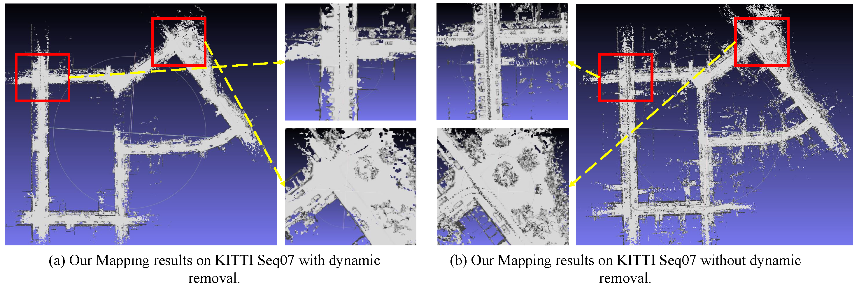
We firstly perform dense mapping on the KITTI dataset. Seq 07 is used for evaluation. The mapping results of our method with and without dynamic removal (unstable voxel removal) are shown in Figure 4. The results demonstrate that the ghost area generated by dynamic objects can be effectively removed by filtering unstable voxels in our method. However, part of static areas, which are not sufficiently observed, are also misclassified as unstable and excluded in the final dense model. The mapping results of the baselines are shown in Figure 5. We can tell that our dense model is superior to them in terms of mapping quality. There are lots of holes in their models. One critical issue is that we take one LiDAR scan from every two scans for dense mapping. The other scan is used for later testing. Such a mechanism means that their systems do not obtain enough LiDAR points to estimate the surface model smoothly. Both their key mechanisms, including the Gaussian Process-based surface model and TSDF computation, require a large number of points to obtain accurate surface parameters estimation. Our method, which is based on point marching cube, is more robust to the scale of LiDAR points and can generate a more accurate map model.

Secondly, we perform dense mapping on the MaiCity dataset. Seq 01 is used for evaluation. The mapping results are shown in Figure 6. From the mapping results of SLAMesh, we can tell that there exists discontinuity between local mesh faces. The reason is that SLAMesh only performs surface estimation and face generation inside each occupied voxel. Surface estimation across voxels is neglected. In our method, face vertices are generated by interpolation on each edge according to the SDF values of cube vertices.

Thirdly, we perform dense mapping on the Stevens-VLP16 dataset. The mapping results are shown in Figure 7. LiDAR points are sparser in this dataset and thus bring more challenges for dense mapping. Our method is still superior to the baselines.

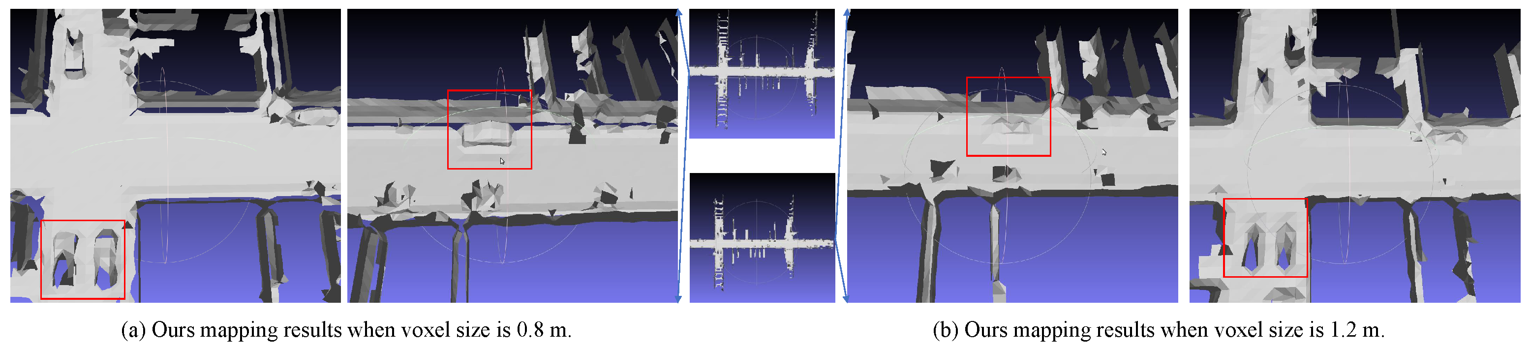
We also perform an ablation study of the mapping performance with regard to voxel size. The results are shown in Figure 8. We can tell that the dense model is blurred when a large voxel size is set. When a large voxel is used, the generated faces within a cube tend to approximate the surface with large errors. Thus, we should set an appropriate voxel size to balance the mapping efficiency and precision.

5.4.4. Quantitatively Comparison

The quantitative evaluation results are shown in

Table 5. The evaluation results ($\mu$, $\sigma$) of the dense mapping model. $\mu$ denotes the mean value and $\sigma$ denotes the standard variance [m].

	KITTI	MaiCity	Stevens
Ours	(0.03, 0.03)	(0.01, 0.16)	(0.01, 0.03)
SLAMesh	(0.11, 0.09)	(0.03, 0.23)	(0.05, 0.17)
VDBFusion	(0.09, 0.12)	(0.03, 0.31)	(0.05, 0.20)

. Our method is more precise than the baselines. The test point cloud map is constructed by aggregating the LiDAR scans collected from different viewpoints. Small errors indicate that the test point cloud map can well match the dense model. The reasons leading to a large matching error are discussed as follows. Firstly, in unstructured areas, the point cloud is unorganized. Surface approximation based on triangle face set still has errors. Secondly, due to the LiDAR points’ sparsity and noise, surface parameter estimation also still has errors, leading to wrong estimation of the zero-value surface. Thirdly, some voxels are not sufficiently activated, which leads to holes in the dense model.

Standard variance is another important index indicating the dense map quality. A large standard variance indicates that there exist a large number of testing points with large matching errors. From Table 5, we can tell that our method is superior to the baselines in terms of the proposed evaluation criterion. Notice that this is achieved under the condition that our voxel size is larger than that in the baselines.

5.4.5. Efficiency Analysis

The computational time cost of each method on KITTI Seq 07 is shown in

Table 6. Time costs of the dense mapping methods [ms].

	t_compute_normal	t_overlap_region	t_match_points	t_gp/t_imls	t_rt	t_update	t_draw_map	t_averaged
Ours	20.49	1.37	0.0	27.29	25.46	1.39	289.39	90.46
SLAMesh	0.0	8.34	21.00	47.38	17.89	4.87	179.21	108.43
VDBFusion	-	-	-	-	-	-	-	118.47

. The definitions are presented as follows. $t\_compute\_normal$ denotes the time to compute the normal of LiDAR points, which is only required in the IMLS-based algorithm in our method. $t\_overlap\_region$ denotes the time cost to compute the overlapping voxels between the current scan and the global map. $t\_overlap\_region$ denotes the time cost to obtain point correspondences. $t\_gp$ denotes the Gaussian Process time cost in SLAMesh and $t\_imls$ denotes the IMSL-based voxel SDF maintenance. $t\_rt$ denotes the registration time cost. $t\_update$ denotes the time cost of updating the global map. These modules are implemented every frame. $t\_draw\_map$ denotes the time cost to generate the global mesh model, which is implemented every 20 frames. It is also highly related to the scale of the environment.

In terms of the $t\_averaged$, our method is more efficient. Firstly, instead of using point-to-mesh-based registration, we use distribution-based registration. Thus, we only need to compute the voxel correspondence between the current scan and global map. Thus, $t\_overlap\_region$ and $t\_match\_points$ only take up little time cost in our method, while SLAMesh spends more time on the point matching process.

However, in terms of $t\_rt$, our method uses more time to perform pose estimation optimization, which indicates that the voxel-based constraints are less rigid than point-based constraints and thus makes the optimizer take more time to converge to the optimal solution. In SLAMesh, in terms of $t\_gp$, Gaussian Process-based surface estimation is time-consuming. In our method, the IMLS-based surface representation is implicit and we only update the SDF values of the voxel center. Thus, $t\_imls$ in our method is less than $t\_gp$. Generating the faces of the global map is still time-consuming given the vertices have been estimated. In our method, we traverse all the occupied voxels, formulate a cube, and implement the marching cube algorithm. In SLMesh, all the occupied voxels are traversed and the vertices formulating faces according to a certain rule in each voxel are directly connected. In VDBFusion, the main process is to integrate the LiDAR points into the global TSDF map and update the TSDF voxels using the ray casting algorithm.

Thus, we only present the final averaged time cost of VDBFusion per frame. We can tell that our method is superior to the baselines in terms of average efficiency.

5.5. Full System Evaluation

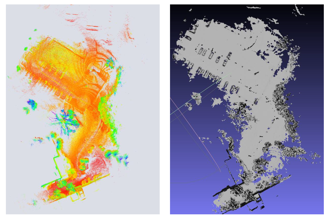
Since we have validated the LiDAR–inertial odometry and TSDF-free dense mapping module, we incorporate them into a full system. The mapping result on the NCLT-20230110 sequence is shown in Figure 9. The two modules are running in different threads. LiDAR–inertial odometry advertises undistorted globally registered LiDAR scans and estimated poses. The mapping module takes the undistorted globally registered LiDAR scans and updates the mesh map in real time. Quantitative evaluation of the mapping quality is presented in

Table 7. The evaluation results ($\mu$ and $\sigma$) of our dense mapping model in LiDAR–inertial datasets.

	NCLT-20130110	LIOSAM-Garden	AVIA-hku-main-building
Ours	(0.01, 0.17)	(0.01, 0.23)	(0.01, 0.18)
FastLIO2-based mapping	(0.09, 0.27)	(0.13, 0.42)	(0.08, 0.32)

. We can tell that the mapping quality can be effectively promoted by replacing FastLIO2 with our odometry.

6. Conclusions

In this paper, we propose a new framework for real-time dense mapping in a local area due to drift errors that cannot be neglected in a long trajectory. We modify the LiDAR–inertial odometry and TSDF-based mapping paradigm. Firstly, normal density is studied in a Gauss–Newton framework. We put weights on residuals given their corresponding normal density. Its effectiveness has been verified in LiDAR–inertial odometry. We will generalize our proposed GN algorithm to other nonliear optimization problems. Secondly, to alleviate the computational burden of constructing TSDF voxels in the whole mapping space, we only construct an SDF vertex in each occupied voxel and formulate an SDF cube when necessary, and it has been proved that such a mechanism benefits the efficiency. The SDF values are computed by an iterative IMLS-based mechanism instead of ray casting. It turns out that our method can use the sparse LiDAR points to estimate the SDF values more accurately and approximate the surface precisely. In the future, we will incorporate a loop closure module into our SLAM system and formulate the global dense map as a graph of the local dense map. Furthermore, we will develop a more efficient and intelligent surface estimator given sparse range and color observations. Scan-to-mesh alignment will be further developed and incorporated.