Abstract
This paper investigates the dynamics of intra-urban real estate cycles by examining the segmentation of real estate markets and their spatial heterogeneity. Despite extensive literature on real estate cycles, insights into intra-urban cycles remain scarce. Utilizing a dataset of over 350,000 apartment sales from 2007 to 2022, first we apply the SKATER (Spatial K’luster Analysis by Edge Tree Removal) algorithm to delineate the city into six distinct clusters, each containing at least 3000 observations, and then analyze the six generated time series of real estate prices. Our findings confirm the hypothesis of market segmentation, revealing significant cyclical differences among the identified submarkets. Analysis indicates that real estate cycles are not uniform across the city. This approach contributes a novel perspective to the existing literature on real estate cycles, emphasizing the need to consider spatial endogenous regimes.
1. Introduction
The real estate market dynamics are highly influenced by various factors, such as government economic policies, macroeconomic cycles, and exogenous shocks. Real estate cycles have been well studied in the literature [1,2,3,4,5], as well as the macro determinants of it among countries [6] and within countries [7,8,9]. Nonetheless, the literature lacks understanding of intra-urban cycles. Are cycles triggered in a specific subset of neighborhoods, or are they generalized processes? What do we consider a booming market that actually takes place in the entire urban agglomeration (city, city-region, or metropolis), or is it just a reflection of the impact of a few centralities in the general real estate price index? Do housing boom and bust processes have contagion effects within an urban agglomeration?
Given that real estate markets are segmented within an urban agglomeration [10,11,12], literature has advanced the understanding of spatial heterogeneity related to housing markets. A distinction can be made between discrete and continuous perspectives on spatial heterogeneity. The continuous approach assumes regression coefficients vary smoothly across locations, while the discrete approach, focused on in this paper, divides data into “spatial regimes”—connected subsets with unique regression coefficients [13]. One good reason for defining spatial regimes in real estate and urban economics analysis is that estimating hedonic price models for each spatial cluster tends to yield better precision to the coefficients and avoids omitted variables, hence, bias.
In this paper, we merge the insights from the literature of spatial regimes on housing markets with those from the literature of real estate cycles to offer an empirical exercise of real estate intra-urban cycles. To proceed with that, we split the studied city into different clusters. Using data from apartments’ transactions of the city of Belo Horizonte, Brazil’s third biggest urban agglomeration, which had a booming real estate market with more than 350,000 sales in the last 15 years, the SKATER (Spatial K’luster Analysis by Edge Tree Removal) algorithm was used to create the sub-markets. To achieve more efficient performance, the city was split into six clusters, with each one having at least 3000 observations. This division was based on different statistical methods, with the scree plot being a key criterion. After that, we built a time series of housing prices for each spatial cluster.
The results corroborated the hypothesis of market segmentation and cyclical differences of the submarkets studied. Furthermore, descriptive analyses brought about evidence that the real estate cycles vary sharply among submarkets.
After this brief introduction, the remainder of the paper is structured as follows. Section 2 brings a brief discussion about the cyclicality of the real estate market. Section 3 presents the historical background and key characteristics of Belo Horizonte`s real estate market. Section 4 and Section 5 outline the methodological approach employed in the study and the dataset utilized. Results and final remarks follow in Section 6 and Section 7.
2. Literature Review
This section offers a brief literature review about the cyclicality of the real estate market. It presents the definition of real estate cycles, discusses its major causes, and mentions its duration.
According to Trojanek (2021) [9], citing a 1994 publication by The Royal Institution of Chartered Surveyors (RICS), real estate cycles are recurring and irregular fluctuations, characterized by variable increases and declines in real estate market activity indicators. Kaiser (1997, p. 233) [1], in highly descriptive work for the US market in a historical perspective, affirmed that “most studies involving real estate cycles define them in terms of vacancy fluctuations around a long-term ‘equilibrium’ line, and analyze the forces that cause new construction, the absorption of space, etc.”. Among these variables, the main focus of our paper is on real estate price, understanding that real estate prices work as a synthesis of economies of agglomeration [14].
Kaiser [1] concluded that boom and bust periods in the real estate market occur as a chain reaction, mainly triggered by periods of high inflation rates, usually reflected by a construction boom. Excessive supply in the upward phase of the cycle would lead to substantial inflation-adjusted price declines in the bust phase. In a broader review article, Duca, Muellbauer, and Murphy (2021) [3] argued that real estate price booms are generally triggered by changes in their fundamentals, such as interest rates, household income, and credit standards. The authors also highlighted the connection of housing markets with credit markets, house price expectations, financial stability, and the wider economy. Shiller (2014) [2] considered that fundamentals—interest rates, population growth, construction costs—are not enough to explain real estate cycles. In his masterpiece, “Irrational Exuberance”, which paved the way for him to receive the Nobel Prize, he emphasized the role of expectations in driving property cycles. Largely shared psychological trends, in other words, speculative behavior of an appreciable number of households, often triggered by media news, plays a very important role in driving real estate prices up and down. This sort of explanation resembles John Maynard Keynes’s concepts on convention and investor behavior (“animal spirits”) to explain the macroeconomic cycles. Edelstein and Edelstein (2020) [5] asserted that historical economic crises are a result of excessive debt, contain a trigger event that creates a “crisis in confidence”; then, created a boom bust cycle with significantly enhanced financial and economic volatilities and generated a boom bust cycle that leads to major contagion effects across the financial and real sectors and spreads internationally. They used this framework to look at the Global Financial Crisis (GFC) of 2007–2008, triggered by the US mortgage market. The role of banks’ lending and other financial institutions’ behavior in driving property cycles has been stressed in the literature, often under the rubric of housing financialization [15,16].
RICS’s definition considers that real estate cycles affect all types of properties simultaneously. Nonetheless, Wheaton (1999) [17] argued that investment levels in certain types of property, such as apartments and industrial areas, are highly correlated with economic factors, and for this reason, there is no inherent cycle or oscillations for these types of property. Instead, there are only reactions at the regional and national levels to economic shocks. In contrast, other property types, such as office spaces, behave differently, as if there were long-term oscillations within their markets [17]. Both Kaiser (1999) [1] and Trojanek [9] considered that the real estate cycles’ duration is less than two decades—18 years for the first author and 12 years for the second.
Fluctuations in real estate prices across countries demonstrate that these cycles vary in terms of duration and magnitude of movements, but most importantly, the economic and demographic factors that influence these cycles and the real estate market are country-specific [9]. However, authors such as [3,5], and [4] have highlighted the existence of international trends in housing markets. This may be due to the increasing connection among countries in the global economy (globalization), both in the sense of international capital flows to national real estate markets and of broader economic trends, such as central banks’ interest rates and rate differentials.
3. A General Description of the Local Real Estate Market
Given the relevance of the historical process of occupation of space to explain the configuration and behavior of the real estate market, this section presents the historical context of Belo Horizonte in relation to this topic. As will be seen, it is possible to note that some features of the first years of occupation of the planned capital remain relevant to explain price and volume differentials in the Belo Horizonte real estate market.
Belo Horizonte, unlike most of the state capitals in Brazil, was born as a planned city, with the specific objective of being the new capital of the State of Minas Gerais, the state which centered the exploration of gold in the 18th Century in Portuguese America. This new city, inaugurated in 1897, was intended to meet the aspirations of the transition from the Empire to the Republic—inaugurated in 1889—under the aegis of positivism. This is reflected in the grid layout of its urban plan for the central area, inspired by Hausmann’s urban plans for Paris and L’Enfant’s for Washington D.C. This planned central area concentrated infrastructure and services, and is separate from the rest of the city by the first Road Ring (the so-called Contour Avenue), and contains the contemporary Central Business District (CDB—the area that mostly concentrate the mass of employments) of the city [18]. Outside the central area, planners aimed suburban districts and further away agriculture zones. North of the central planned area, there is a water stream (Ribeirão Arrudas) that runs from west to east, and the railroad that follows it in this portion of the city. Due to these two barriers, the water stream and the railroad, the Northern areas of the city are historically less valued than those in the Southern areas [19].
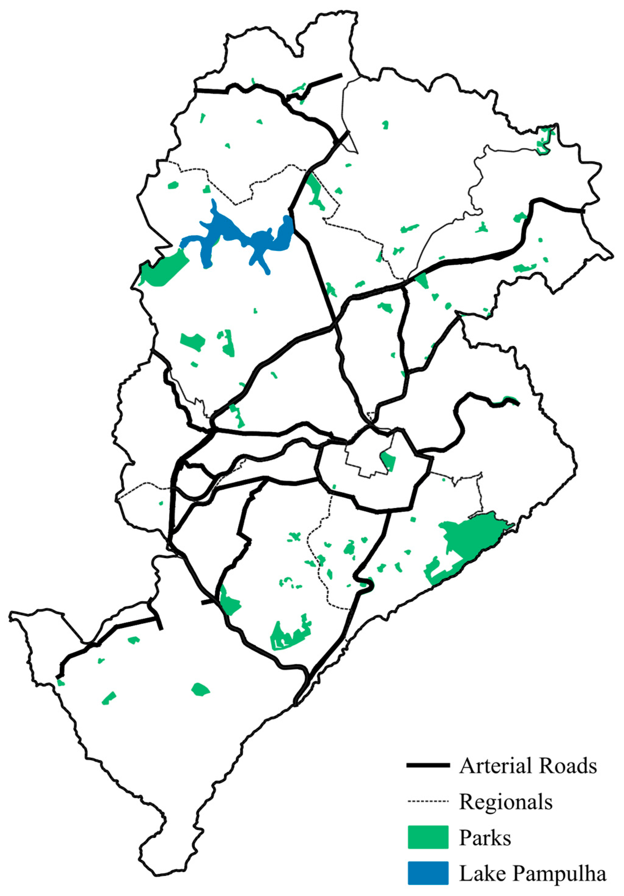
Despite initially being thought of as a political city, Belo Horizonte has undergone massive industrialization throughout the 20th Century, which made it the center of a metropolitan region, nowadays with 5.7 million people, 2.3 million of them living in the municipality of Belo Horizonte, and the remaining population spread across the other 33 municipalities. The industrialization–urbanization processes created vast working-class neighborhoods north and west of the central planned area. The local elites inhabit mainly inside the CBD and have expanded southwards [20]. Eastward expansion has been limited by geographical features, mainly the Serra do Curral, and by the lack of major economic activities. In the Southern portion of this Sierra, there is a large park, one of the main amenities in the municipality of Belo Horizonte. Other relevant amenities are the Municipal Park, located in the central area, and the Pampulha lake, located in the northwest part of the city, surrounded by some large parks, such as the zoo. Figure 1 depicts these features for the municipality of Belo Horizonte. Solid black lines represent arterial roads, the first ring (Contour Avenue) and the second ring (Road Ring). Green areas represent the green parks. The district named “Downtown” is represented by a black light polygon, inside the first ring, although it is important to remember that the CDB encompasses the entire area within the first ring.

Figure 1.
Map of Belo Horizonte—center, main roads, parks, and the lake. Source: Authors.
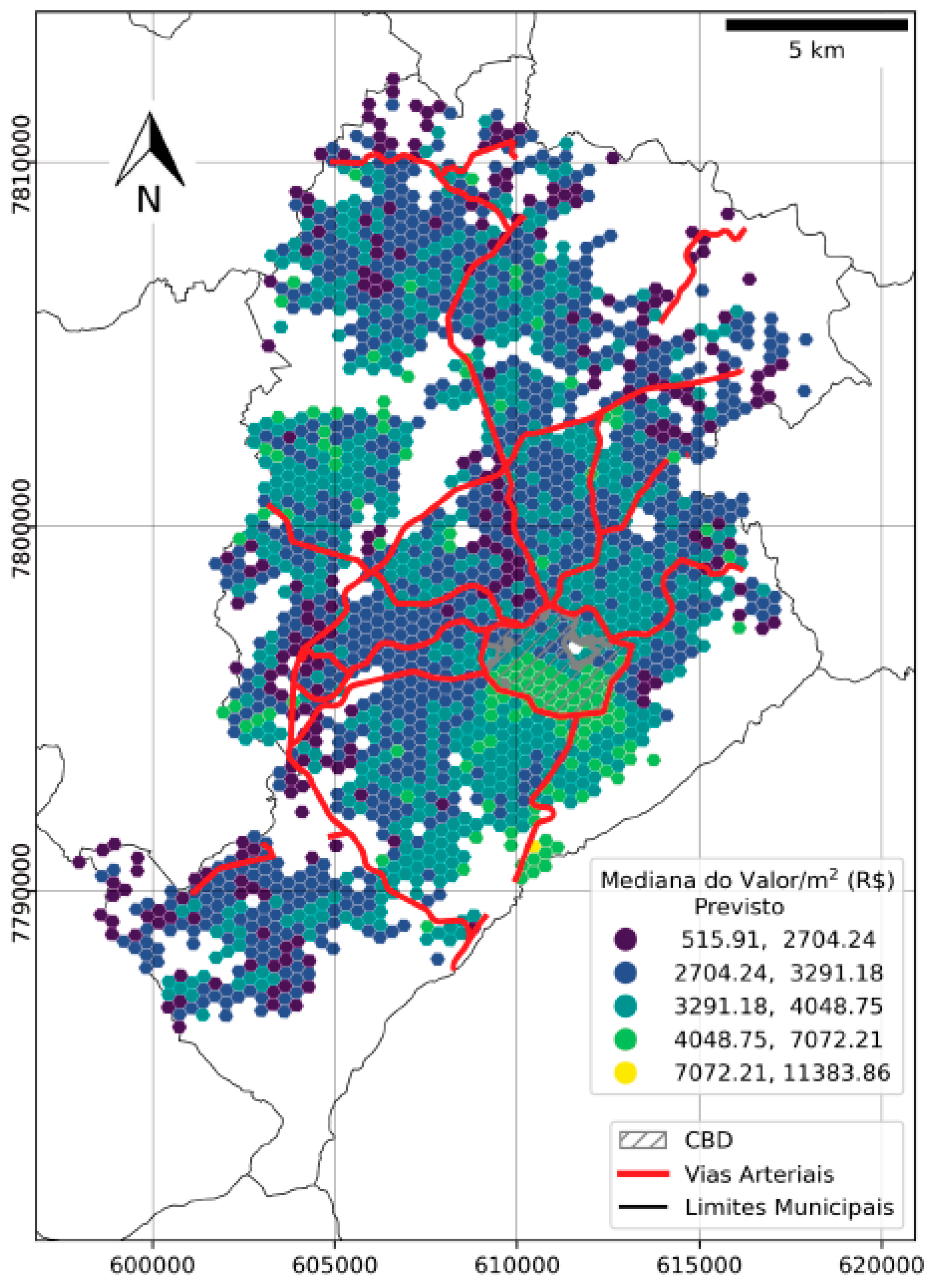
We also offer a view of the local real estate market through the estimated apartment values map, in other words, the bid-rent map estimated by a hedonic price model for all the existing apartments in the city in 2020 [18]. This is represented in Figure 2, in which one sees the concentration of high values in the Southern parts of the map.

Figure 2.
Map of the estimated apartment’s values, main roads, and CBD—Belo Horizonte (2020). Source: [18].
One of the reasons Belo Horizonte has been studied by real estate scholars is that its local government has performed accurate work in making available a high-quality dataset for real estate transactions, based on the local taxes. This dataset is publicly available by request and has been used by scholars in several empirical studies [12,18,21,22,23,24]. Moreover, Belo Horizonte is the third largest metropolis in Brazil, and it is home to many research institutions, a fact that increases the interest on it.
4. Methodology
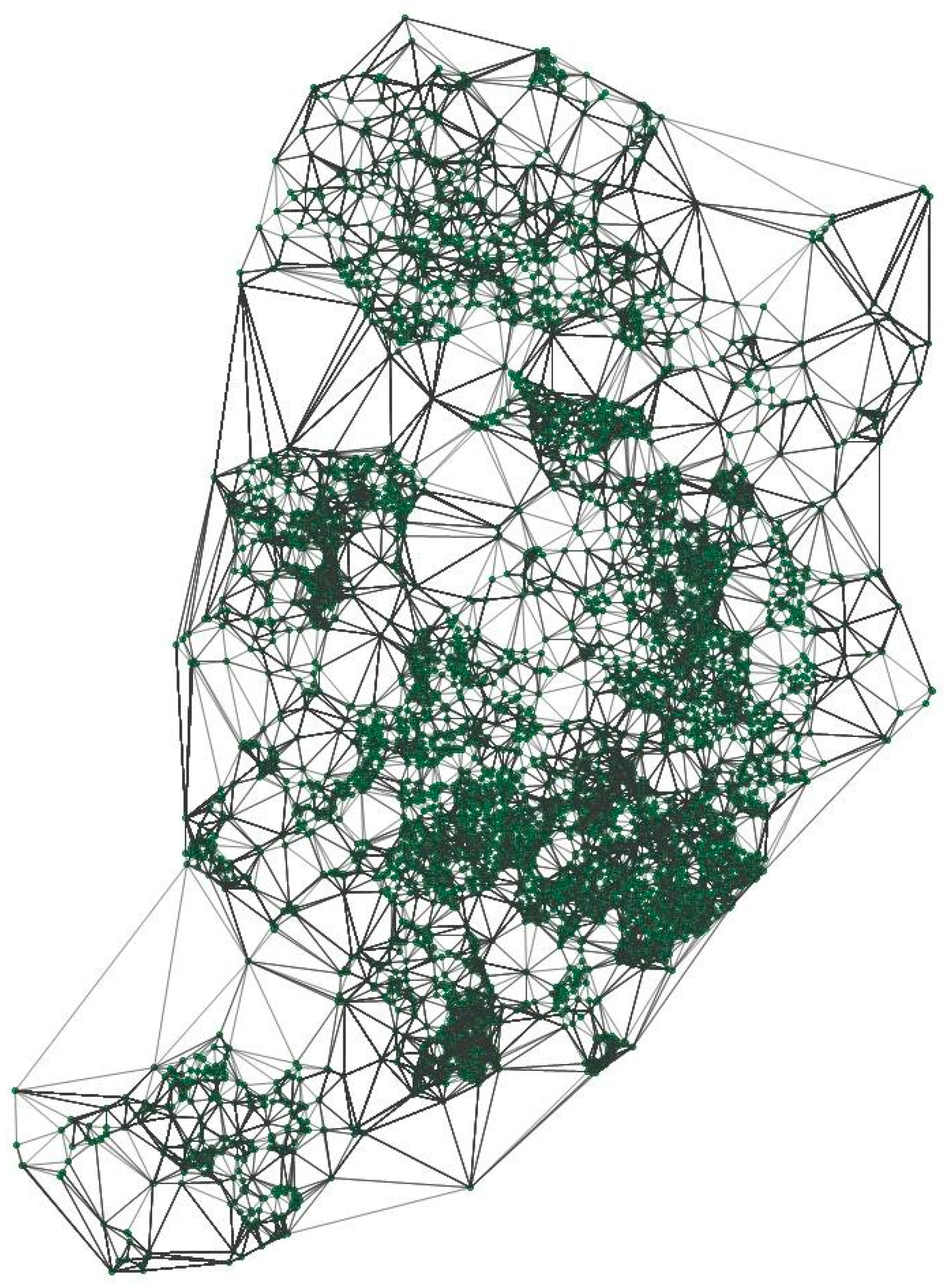
The SKATER (Spatial ‘K’luster Analysis by Tree Edge Removal) technique is used here to create the real estate submarkets within the city. The SKATER regionalization technique, proposed by Assunção et al. (2006) [25], is derived from approaches that include algorithms that involve adjacency relations as restrictions on the clustering process. In other words, this algorithm is a multivariate method that creates groups (clusters) minimizing the within-group dissimilarities and, at the same time, respecting the restriction that these groups need to be continuous. Since spatially restricted clustering algorithms are computationally intensive, [25] performed SKATER, which is computationally more efficient. An important feature of SKATER is that connectivity graphs that capture the adjacency relations between objects are used to create groups, where each object is associated with a vertex and connected by edges to its neighbors, as shown in Figure 3.

Figure 3.
Connectivity graph of apartments’ sales in 2022. Source: Authors.
However, before creating the connectivity graph, the first step of SKATER is to create an n × n spatial weighting matrix, W, whether it is a contiguous matrix, a geographic distance matrix, an inverse distance matrix, or one of the other possible methods [13]. In this paper, a first-order contiguous matrix of the Queen type was chosen. Weighted matrices provide the structure for a graph, where each observation is a node (or vertex) and the edges correspond to non-zero elements in the spatial weighting matrix [13].
After creating the spatial weighting matrix and the connectivity graph, the next SKATER step is the reduced graph using the Minimum Spanning Tree technique. It is important to highlight some concepts of this approach for better understanding. A circuit is a similar path to the first and last vertex of a graph (as shown in Figure 3), while a Tree is a connectivity graph where no circuits occur. A Spanning Tree T of a graph G is a Tree that contains all the vertices of G, where a single path connects any two vertices [25]. Finally, a Minimum Spanning Tree (MST) is a Spanning Tree with the shortest possible path. In other words, in this phase, a path is generated, which connects all spatial elements without a cycle or a circular path occurring, where the optimal path (the path with the lowest cost if we are talking about transportation costs from one location to another) is based on the smallest sum of the dissimilarities (distance) of the edges [13,25]. Therefore, a Minimum Spanning Tree T will have n vertices and n − 1 edge.
The last step to complete SKATER is a “pruning” of the MST, which is the removal of any edge of T, resulting in two different subgraphs of the spatial cluster candidates. Since the graph is based on contiguity, each resulting subgraph will also have elements that are spatially contiguous [13].
As in any process of creating submarkets through SKATER or any other form of delimitation, it is first necessary to determine which variable or group of variables is used to inform its creation. Therefore, the SKATER present in this study was made using the GeoDA (version 1.22.0.10) software, and the variable apartment prices/m2 was used as the key variable.
After creating the clusters, representing each real estate submarket of the city, we use typical descriptive statistical analysis to describe these data. Moreover, we present time-series plots on the average price per square meter of each cluster to illustrate some evidence of intra-urban real estate cycles.
5. Data
The methodology used to achieve the final objective of this work was, first, to obtain the database. The data used were the records of the Real Estate Transfer Tax (RETT) relating to real estate transactions in Belo Horizonte between 2007 and 2022. To ensure greater consistency and quality of the information, the data underwent a cleaning process. The original database, which contains transactions between 2007 and 2023 for the city of Belo Horizonte, contains 315,779 observations, but after cleaning, the final database now has 265,775 observations. The database was cleaned as follows: (i) 1170 observations from the Acquired Constructed Area variable, with values smaller than 10 m2 and larger than 1000 m2, were removed; (ii) 1095 observations from the Declared Value variable, with values smaller than BRL 999.00 and larger than BRL 30,000,000.00, were removed; (iii) 1483 observations from the Value/m2 variable, with values smaller than 50 BRL/m2 and larger than 40,000 BRL/m2, were removed; (iv) 33,281 observations from the Launch State variable, with values classified as “Null Value”, “Cancelled” or “Deactivated”, were removed; (v) 19 observations from the Year of Construction variable, with values smaller than 1990, were removed; (vi) 1386 observations with incorrect coordinates were removed; and (vii) 11,570 observations of apartments transacted in 2023 were removed, as the study will only include observations up to the year 2022.
6. Results
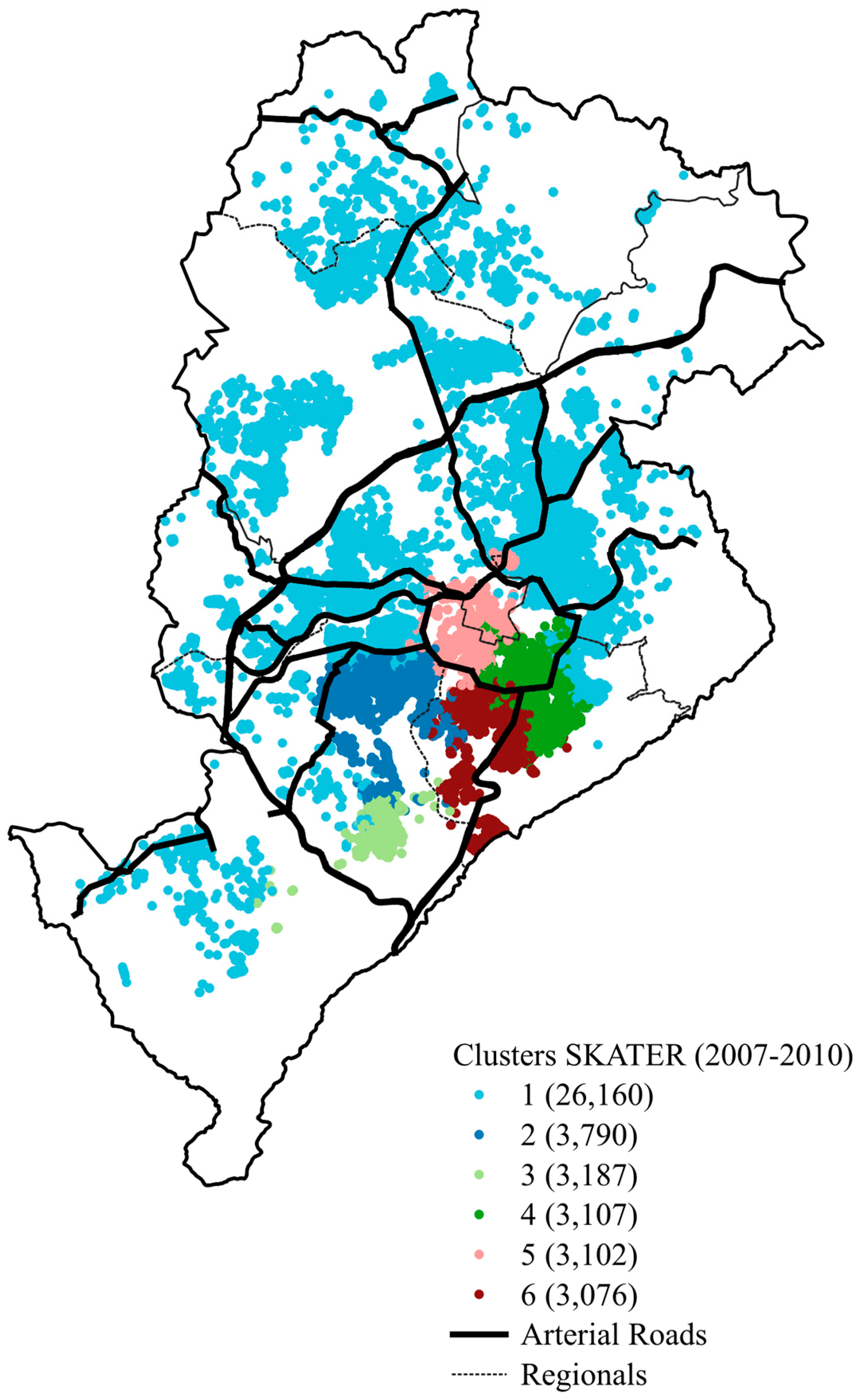
One possibility of the SKATER algorithm is its ability to set a minimum number of observations for each cluster that is created. Based on this possibility, we tested different approaches to achieve a good fit—both with a predefined minimum number of observations for each cluster and with a free minimum number that the algorithm itself chooses. In this manner, with six clusters, we found a good fit, with reasonable adherence to the literature about real estate markets in the studied city [18,26,27,28] and the researchers’ knowledge of the market. Each cluster has a restriction of a minimum of 3000 observations, as shown in Figure 4.
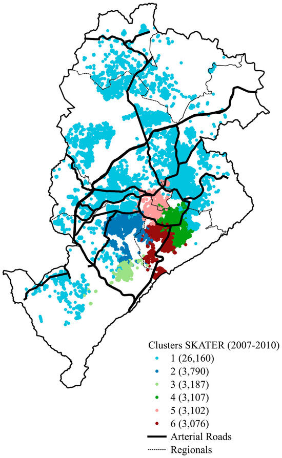
Figure 4.
SKATER with a minimum of 3000 observations (2007–2010). Source: Authors.
Clustering analysis typically does not require statistical significance, given that this method aims to create separate groups in a descriptive manner. This does not mean that it is not possible to infer the statistical difference between clusters, but that it is to say that authors usually do not make use of additional methods to discuss the statistical significance of each cluster. Nonetheless, scholars usually use the following metrics to explore the quality of the partition made by the clustering analysis: Since the total variance equals the sum of the within-group variances and the total between-group variance, a common criterion is to assess the ratio of the total between-group variance to the total variance. A higher value for this ratio suggests a better separation of the clusters.
In our study, this ratio was 0.34, which is a fairly good separation. To check the robustness of this metric, we run the SKATER algorithm with several different spatial matrices, obtaining, among these trials, a ratio of 0.70 using a K-nearest neighbors matrix. However, this approach resulted in a much worse spatial configuration of the clusters, spatially spread and superimposed, hurting the very reason to use a spatial clustering analysis—obtaining a group of contiguous sub-groups of real estate markets. For this reason, we kept using the original Queen Matrix.
Figure 4 shows SKATER using data from 2007 to 2010 for the city of Belo Horizonte. It is important to note that a neighborhood or district does not necessarily have only one type of classification, i.e., a given district may have apartments in Clusters 1 and 2, for example. It is worth noting that Cluster 1 (middle-income, peripherally located) is the largest and covers all the “peripheries” of the city, understood as the areas outside the originally planned region and the first road ring. All the following interpretation of the socioeconomic characteristics of the clusters follows [26].
Cluster 2 (middle-income, semi-peripherally located) has almost all transaction points in neighborhoods in the Western districts, limited by two arterial roads, in the north and in the western portions of this cluster. It includes districts such as Buritis, Grajaú, Nova Suíssa, and close districts, and a few neighborhoods in the Central-South region, such as Luxemburgo and Vila Paris. It aggregates middle-class neighborhoods.
Cluster 3 (middle-income, southwestern-located) covers three regions in its apartment sales: Barreiro, West, and Central-South. However, most of its transactions are in the districts of Buritis and Estoril, in the southwestern region of Belo Horizonte, middle-class neighborhoods of relatively new apartment buildings.
Cluster 4 (high-income, centrally located), in turn, is located basically in the Central-South region and in some Eastern portions of the city that go upwards the Serra do Curral. It is an upper-middle-class and elite area and aggregates districts such as Savassi, Funcionários, Santa Efigênia, and Serra, which are historically associated with the bureaucratic and military elites.
Cluster 5 (high-income, centrally located) also has a large number of apartment transactions in districts in the Central-South region. These districts are, for example, Barro Preto and Boa Viagem, but most transactions are in the Downtown, Lourdes, and Santo Agostinho districts. It aggregates elites and upper-middle-class neighborhoods, and it is mostly located just north of the Downtown, being historically associated with the bourgeoisie of the city.
Finally, Cluster 6 (upper middle-income, suburban) is located predominantly in the southwest region of the Center-South region, and some districts that encompass this group are Sion, Santa Lúcia, Santo Antônio, and Belvedere. These are upper-middle-class and elite areas, concentrating newer apartment clusters than the traditional areas in the first ring. Especially, the district called Belvedere stands out as the locus of the city’s new riches, exhibiting high-rise apartment buildings on the southern border of Belo Horizonte.
With the clusters formed, it was possible to create polygons from the points of each grouping. This step is useful to classify the points of the other years of the sample according to how they “fall within” the clusters formed, so that the intra-urban dynamics of these clusters can be analyzed over time. As can be seen in Figure 4, all the clusters had small parts overlapping other clusters. Given this problem, it was necessary to cut parts of some groupings.
The criterion used was the cut based on the total area of the clusters in km2, as shown in Table 1. If two groups overlap, the group with the largest area will have its overlapping parts cut. Given this criterion, only Clusters 3 and 5 did not have parts of their polygons cut. It is worth mentioning that this heuristic was designed and operationalized specifically for this work and is not based directly on methodologies previously known through the literature.

Table 1.
Area in km2 of the formed clusters.
After creating the polygons, it is possible to relate the apartments from the other years in the database (2011–2022) to the clusters created through the SKATER algorithm (2007–2010, Figure 5). Using this approach, it is possible to capture the behavior of the average apartment’s characteristics over time in the areas formed by the SKATER, creating a time series for each cluster. It is important to note that the polygons, when placed together, do not represent the map with the administrative limits of the city, but rather the area in which records of transacted apartments are found. This reflects the segmentation of real estate submarkets within the city.
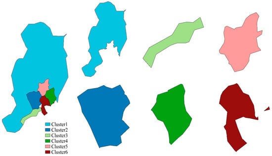
Figure 5.
Polygons based on SKATER (2007–2010). Source: Authors.
We present below descriptive statistics for each of the submarkets created for the city. Note that from this point onwards, all prices are deflated based on the 2011 Broad Consumer Price Index. Table 2, therefore, shows the real sales prices of apartments.
Table 2.
Descriptive statistics by cluster—real values per square meter (m2) in BRL of 2011.
Table 2 shows the deflated sales prices of apartments. The general cycle has a boom period (2011–2014, which actually started in 2007) followed by a bust period (2014–2022) (see [29] for Brazil; [22] for this city). In relation to the years 2012 and 2013, all groups achieved their largest positive variations in average prices, but there were considerable differences between them. Cluster 3 (middle-income, southwestern-located) presented the smallest positive variation among the groups for both years, 8.55% in 2012 and 4.33% in 2013. The largest positive variation in 2012 was in Cluster 5 (high-income, centrally located), with 22.29%, and in 2013, it was in Cluster 1 (middle-income, peripherally located), with 15.45%. All groups showed a downward trend in apartment prices, either from 2014, with groups 2 (middle-income, semi-peripherally located) and 3, or from 2015 with groups 1, 4, 5, and 6. This finding is interesting in noting that the bust cycle does not start at the same time in all clusters, but first in two clusters. These two clusters (2 and 3) are composed of relatively newer high-rise apartment buildings in the upper-middle class, located outside the city’s first ring circle. One may suppose that this kind of submarket tends to be more volatile than more consolidated traditional upper-class submarkets.
Most groups had negative variations from 2015 until 2022, the last year of the period analyzed. There are, however, four exceptions: In 2017, groups 1, 3, and 4 presented an increase of 0.18%, 1.24%, and 0.50%, respectively, in apartment prices, and in 2022, group 6 (upper middle-income, centrally located) had a positive variation of 0.92%. In total, there were 19 positive variations and 45 negative variations for the average apartment prices.
Regarding the average values, groups 4 (high-income, centrally located) and 5 (high-income, centrally located) are where the most expensive apartments are located during the period analyzed. On the other hand, groups 1, 2, and 3 are the cheapest. For the groups that began to see a drop in property prices in 2015, the highest maximum value was observed in the previous year. The same logic is seen in the groups that began to suffer from price drops in 2014, which in turn presented the highest maximum values in 2013.
Based on cumulative variations, Table 3 shows two different types of growth rates in the average apartment prices analyzed during the period: the geometric growth rate and the cumulative growth rate. It contains three different time intervals: 2011–2014, 2015–2022, and 2011–2022. In the simplest possible way, the geometric growth rate shows the annual growth rate of property prices in the six clusters created. Negative variations were expected, given the results presented in Table 2. For the time span 2011–2022, the most negative result belongs to Cluster 3 (middle-income, southwestern-located), with properties losing 2.07% of their real value annually. For the same time span, Cluster 1 is the one that had the lowest loss of value on average, which showed a drop of −0.20% annually. The first time span shows how real estate prices were growing strongly, such as 12.59% and 13.66% for Clusters 1 (middle-income, peripherally located) and 5 (high-income, centrally located), respectively. In addition to being the group that presented the largest drops, Cluster 3 was also the group that presented the smallest growth in this first period. In the second period (2015–2022), it shows how apartment prices fell. It is interesting how all groups presented very similar drops. Cluster 5 was responsible for presenting the largest drop in rates for this second period. This group, therefore, presented the highest growth rates for the years 2011–2014 and the largest drop rates for the years 2015–2022.
Table 3.
Geometric growth and cumulative growth rate of clusters—deflated real estate prices—(2011–2022).
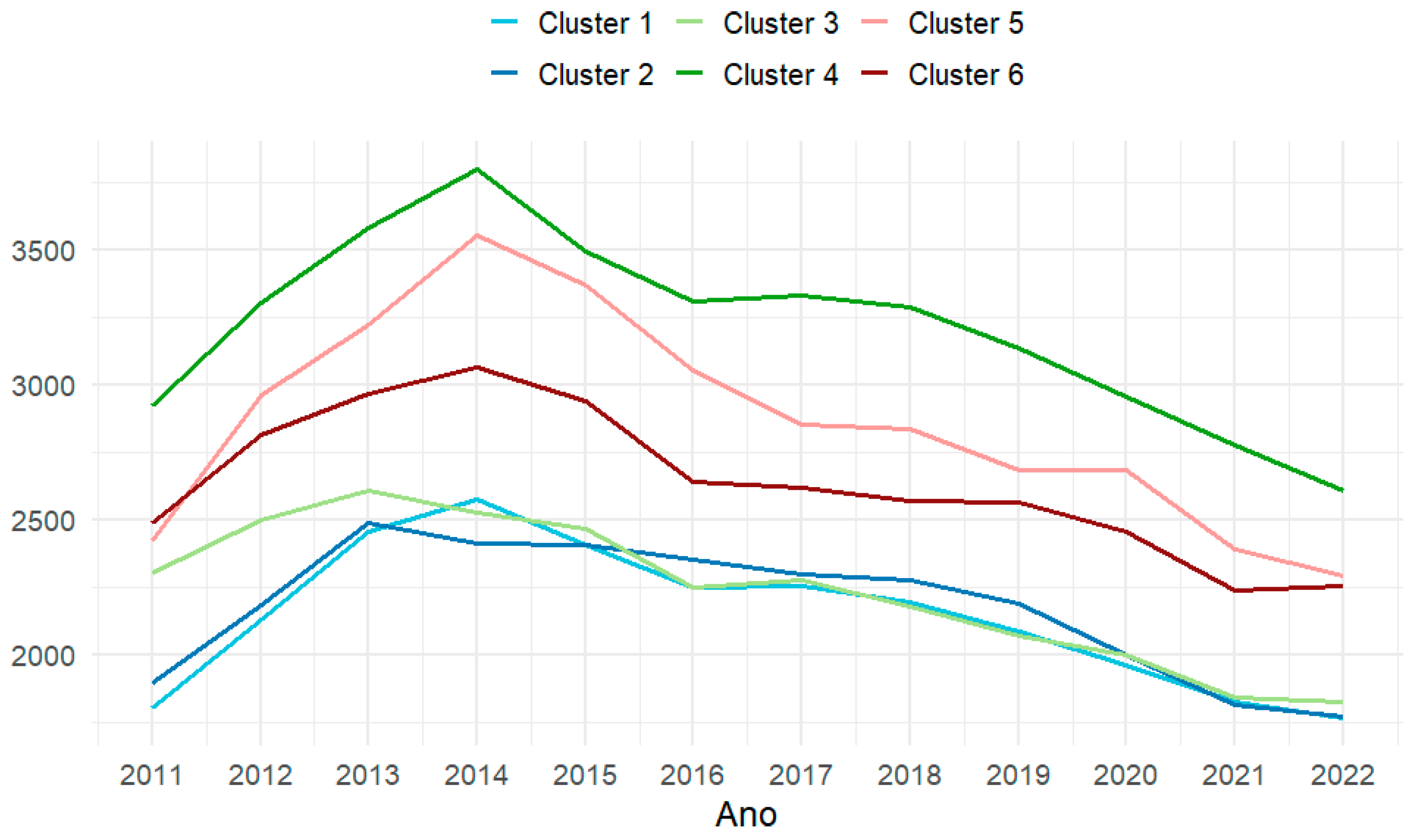
The cumulative growth, on the other hand, mainly shows a percentage variation in the averages between the beginning and the end of the period. In conjunction with Figure 6, it is interesting to note how Cluster 3 was close to Clusters 5 and 6 in 2011; however, having lost more than 20% of its real value, in 2022, Cluster 3 was very close to Clusters 1 (middle-income, peripherally located) and 2 (middle-income, semi-peripherally located).
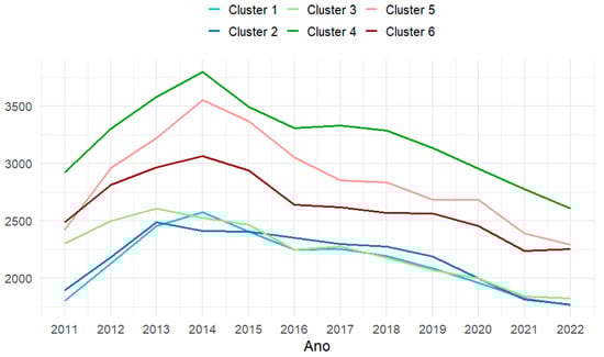
Figure 6.
Average prices by cluster. Source: Authors.
Figure 6 provides a better view of Table 2. It is clear that Cluster 4 (high-income, centrally located) is the region with the highest average prices over the years. Although Cluster 5 (high-income, centrally located) was close to Cluster 4 between 2014 and 2016, its prices differed significantly from 2016 onwards. Furthermore, it is also possible to observe that Cluster 5 is closer to being similar to Cluster 6 (upper middle-income, suburban) than to Cluster 4. Furthermore, Figure 6 also shows how the price of the first three clusters became very close to each other, especially in the last years of the data (2020–2022).
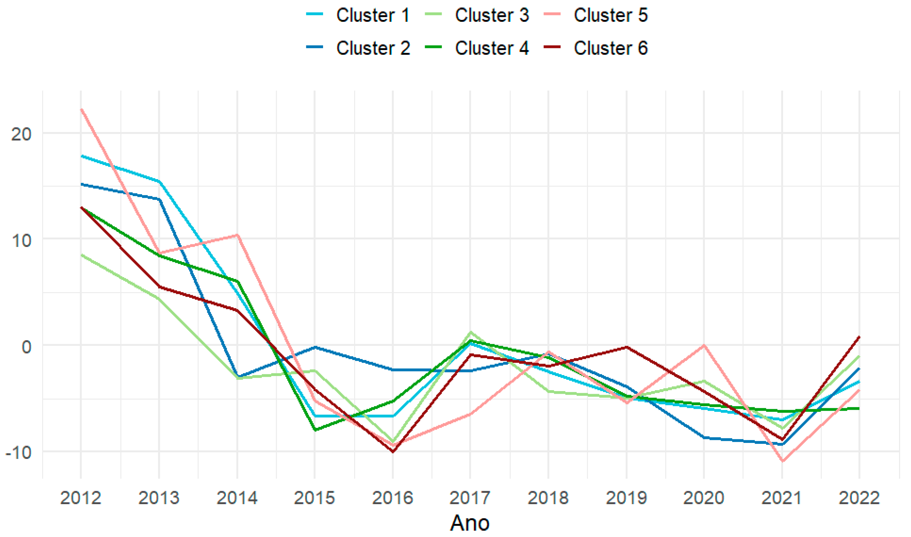
Figure 7 shows the variations in average prices over the years. As can be seen, the variations in average prices are slightly similar between the groups, but an important point to be highlighted in this graph is how the variations are positive and relatively high in 2012 and 2013, and how they start to become negative from 2014 and 2015, depending on the group viewed. Note that the variations are always between −10% and 0%, with a few exceptions when this margin is exceeded.
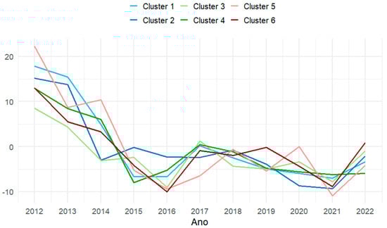
Figure 7.
Percentage of variation in average prices by cluster. Source: Authors.
7. Final Remarks
This paper explored the heterogeneity of real estate markets within the city—a feature that defines endogenous spatial regimes and their real estate submarkets in cities—and used this fact to investigate intra-urban real estate cycles. To the best of our knowledge, this is a new approach to the real estate cycles literature [1,2,3,5] and highlights the importance of understanding different paths and trends in these cycles.
We benefit from a rich dataset, containing more than 350,000 observations of sales prices from 2007 to 2022. Moreover, new spatial techniques, such as the SKATER methodology applied to the study of real estate markets [13], help to advance our understanding of intra-urban real estate cycles.
The descriptive analysis offered here shows that, if we properly divide the city’s submarkets, we are able to identify its real estate submarkets and then create time series to study them. In this paper, we found that there are important variations over time among different submarkets.
Future research must use causal estimation techniques to clearly identify which sort of variables explain these differences in a city’s submarkets. Two possibilities are the vector autoregression (VAR) approach and the local projection approach, both currently used in macroeconomic time-series studies. This may illuminate what drives real estate cycles on a very detailed spatial scale, strengthening the comprehension of urban economists, planners, architects, geographers, engineers, real estate appraisers, and all those who are interested in understanding this.
Author Contributions
All authors contributed equally to this work. All authors have read and approved the final version of the manuscript. All authors have read and agreed to the published version of the manuscript.
Funding
This research was partially funded by CAPES/Brazil by its Master’s Program grants to UFSJ and by the Universal Demand Grant of the Brazil’s National Council for Scientific and Technological Development, and the APC was funded by Società Italiana di Estimo e Valutazione (SIEV).
Institutional Review Board Statement
Not applicable.
Informed Consent Statement
Not applicable.
Data Availability Statement
Not applicable.
Conflicts of Interest
The authors declare no conflicts of interest.
References
- Kaiser, R. The Long Cycle in Real Estate. J. Real Estate Res. 1997, 14, 233–257. [Google Scholar] [CrossRef]
- Shiller, R.J. Irrational Exuberance, 3rd ed.; Princeton University Press: Princeton, NJ, USA, 2014. [Google Scholar]
- Duca, J.V.; Muellbauer, J.; Murphy, A. What Drives House Price Cycles? International Experience and Policy Issues. J. Econ. Lit. 2021, 59, 773–864. [Google Scholar] [CrossRef]
- Almeida, R.P. Cycles, Trends, Disruptions: Real Estate Centrality on the Global Financial Crisis, COVID-19 Pandemic, and New Techno-Economic Paradigm. Real Estate 2025, 2, 1. [Google Scholar] [CrossRef]
- Edelstein, M.D.; Edelstein, R.H. Crashes, Contagion, Cygnus, and Complexities: Global Economic Crises and Real Estate. Int. Real Estate Rev. 2020, 23, 311–336. [Google Scholar] [CrossRef] [PubMed]
- Aizenman, J.; Jinjarak, Y. Current Account Patterns and National Real Estate Markets. J. Urban Econ. 2009, 66, 75–89. [Google Scholar] [CrossRef]
- Zhang, H.; Li, L.; Hui, E.C.-M.; Li, V. Comparisons of the Relations between Housing Prices and the Macroeconomy in China’s First-, Second- and Third-Tier Cities. Habitat Int. 2016, 57, 24–42. [Google Scholar] [CrossRef]
- DeFusco, A.; Ding, W.; Ferreira, F.; Gyourko, J. The Role of Price Spillovers in the American Housing Boom. J. Urban Econ. 2018, 108, 72–84. [Google Scholar] [CrossRef]
- Trojanek, R. Housing Price Cycles in Poland—The case of 18 provincial capital cities in 2000–2020. Int. J. Strateg. Prop. Manag. 2021, 25, 332–345. [Google Scholar] [CrossRef]
- Furtado, B.A. Neighbourhoods in Urban Economics: Incorporating Cognitively Perceived Urban Space in Economic Models. Urban Stud. 2011, 48, 2827–2847. [Google Scholar] [CrossRef]
- Bhattacharjee, A.; Castro, E.; Maiti, T.; Marques, J. Endogenous Spatial Regression and Delineation of Submarkets: A New Framework with Application to Housing Markets: Endogenous Spatial Regression and Delineation of Submarkets. J. Appl. Econ. 2016, 31, 32–57. [Google Scholar] [CrossRef]
- Almeida, R.P.; Monte-Mór, R.L.M.; Amaral, P.V.M. Implosão e Explosão Na Exópolis: Evidências a Partir Do Mercado Imobiliário Da RMBH. Nova Econ. 2017, 27, 323–350. [Google Scholar] [CrossRef]
- Anselin, L.; Amaral, P. Endogenous Spatial Regimes. J. Geogr. Syst. 2024, 26, 209–234. [Google Scholar] [CrossRef]
- Caragliu, A. Cities and the Urban Land Premium. Reg. Stud. 2016, 50, 374–375. [Google Scholar] [CrossRef]
- Rolnik, R. Late Neoliberalism: The Financialization of Homeownership and Housing Rights. Int. J. Urban Reg. Res. 2013, 37, 1058–1066. [Google Scholar] [CrossRef]
- Ryan-Collins, J.; Llyod, T.; McFarlane, L. Rethinking the Economics of Land and Housing, 1st ed.; Zed Books: London, UK, 2017; Volume 1. [Google Scholar]
- Wheaton, W.C. Real Estate “Cycles”: Some Fundamentals. Real Estate Econ. 1999, 27, 209–230. [Google Scholar] [CrossRef]
- Patrício, P.; Tonucci, J.; Almeida, R. Mercado Imobiliário e Estrutura Urbana: Uma Análise Da Formação de Preços de Lotes Vagos e Apartamentos Em Belo Horizonte (2009–2020). Available online: https://repositorio.ufmg.br/handle/1843/44106 (accessed on 16 April 2025).
- Villaça, F.J.M. O Espaço Intra-Urbano No Brasil, 2nd ed.; FAPESP, Lincoln Institute: São Paulo, SP, Brazil, 2001. [Google Scholar]
- Almeida, R.; Patrício, P.; Brandão, M.; Torres, R. Can Economic Development Policy Trigger Gentrification? Assessing and Anatomising the Mechanisms of State-Led Gentrification. Enviorn. Plan A 2022, 54, 84–104. [Google Scholar] [CrossRef]
- Paixão, L.A.R.; Luporini, V. A valorização imobiliária em Belo Horizonte, 1995–2012: Uma análise hedônica-quantílica. Nova Econ. 2019, 29, 851–880. [Google Scholar] [CrossRef]
- Paixão, L.A.R.; Luporini, V. Índice de preços hedônicos para apartamentos: Uma aplicação a dados fiscais de Belo Horizonte, 1995–2012. Econ. Soc. 2020, 29, 967–993. [Google Scholar] [CrossRef]
- Almeida, R.; Brandão, M.; Torres, R.; Patrício, P.; Amaral, P. An Assessment of the Impacts of Large-Scale Urban Projects on Land Values: The Case of Belo Horizonte, Brazil. Pap. Reg. Sci. 2021, 100, 517–559. [Google Scholar] [CrossRef]
- Nabuco, A.L. Land tenure, construction companies, real estate and financial capital. Who owns the city of Belo Horizonte? Rev. Bras. Estud. Urbanos E Reg. 2019, 21, 567–585. [Google Scholar] [CrossRef]
- AssunÇão, R.M.; Neves, M.C.; Câmara, G.; Da Costa Freitas, C. Efficient Regionalization Techniques for Socio-economic Geographical Units Using Minimum Spanning Trees. Int. J. Geogr. Inf. Sci. 2006, 20, 797–811. [Google Scholar] [CrossRef]
- Almeida, R.P. Implosão e Explosão na Exópolis: Evidências a partir do Mercado Imobiliário da RMBH. Master’s Dissertation, Universidade Federal de Minas Gerais, Centro de Desenvolvimento e Planejamento Regional, Belo Horizonte, Brazil, 2015. [Google Scholar]
- Furtado, B.A. Mercado Imobiliário e a Importância Das Características Locais: Uma Análise Quantílico-Espacial de Preços Hedônicos Em Belo Horizonte. Rev. Análise Econôm. 2007, 25, 71–98. [Google Scholar] [CrossRef]
- de Aguiar, M.M.; Simões, R.; Golgher, A.B. Housing Market Analysis Using a Hierarchical–Spatial Approach: The Case of Belo Horizonte, Minas Gerais, Brazil. Reg. Stud. Reg. Sci. 2014, 1, 116–137. [Google Scholar] [CrossRef]
- Mioto, B.T. Dinâmica econômica e imobiliária: Periodização dos macrodeterminantes dos anos 2000 e 2010. Cad. Metrop. 2022, 24, 15–32. [Google Scholar] [CrossRef]

Disclaimer/Publisher’s Note: The statements, opinions and data contained in all publications are solely those of the individual author(s) and contributor(s) and not of MDPI and/or the editor(s). MDPI and/or the editor(s) disclaim responsibility for any injury to people or property resulting from any ideas, methods, instructions or products referred to in the content. |
© 2025 by the authors. Licensee MDPI, Basel, Switzerland. This article is an open access article distributed under the terms and conditions of the Creative Commons Attribution (CC BY) license (https://creativecommons.org/licenses/by/4.0/).