Towards Early-Stage Corrosion Prediction Using UHF RFID Measurements: A Machine Learning Feasibility Study

Abstract

Conventional corrosion monitoring techniques often require costly instrumentation and direct access to structures, limiting their suitability for long-term monitoring. This study presents a machine learning feasibility study for early-stage corrosion detection using Ultra-High Frequency (UHF) Radio Frequency Identification (RFID) measurements. Machine learning algorithms were applied to a previously published RFID corrosion dataset obtained from steel specimens exposed to marine atmospheric corrosion for 0, 1, 3, and 6 months. RFID-derived features, including Analogue Identifier (AID), forward power, frequency, phase, and backscattered power, were analysed using unsupervised and supervised learning methods. For corrosion-stage discrimination, Density-Based Spatial Clustering of Applications with Noise (DBSCAN) achieved an Adjusted Rand Index (ARI) of 1.00, a Normalised Mutual Information (NMI) score of 1.00, and a Silhouette score of 0.790. For nominal corrosion-thickness state estimation, a Random Forest regressor achieved an $R^2$ of 1.00, RMSE of 1.34 µm, and MAE of 0.21 µm under 15-fold cross-validation. Additional Leave-One-Sample-Out (LOSO) validation using readcount-based measurement-event groupings yielded an RMSE of 0.12 µm and an $R^2$ of 1.00. These results reflect nominal corrosion-thickness state estimation from repeated measurements on a single physical specimen per corrosion stage. SHAP analysis identified forward power and AID as the dominant predictive features. The results demonstrate the potential of RFID-enabled machine learning for early-stage corrosion assessment and provide a foundation for future experimental validation.

1. Introduction

Structural Integrity Evaluation (SIE) and Structural Health Monitoring (SHM) are essential for maintaining large-scale infrastructure and industrial assets, especially metallic structures that are prone to widespread degradation due to corrosion. Corrosion is a major threat that can cause catastrophic structural failure if not detected early. The crucial window for effective intervention and condition-based maintenance is during early-stage corrosion, which is characterised by pitting, increased surface roughness, and the growth of a corrosion layer before significant metal loss occurs [1,2].

Traditional electromagnetic Non-Destructive Testing and Evaluation (NDT&E) methods, such as Pulsed Eddy Current (PEC) and Eddy Current Pulsed Thermography (ECPT) [3,4,5], are proven techniques for corrosion detection and characterisation. However, a fundamental limitation of these conventional approaches is the requirement for complex, bulky, and often expensive systems that necessitate wired connections or physical access, rendering them unsuitable for permanent, distributed monitoring across extensive structures, such as railway tracks or bridges [2]. Therefore, an effective alternative solution is required to ensure structural safety and reliability. Ultra-High Frequency (UHF) Radio Frequency Identification (RFID) systems, specifically utilising the Tag-Antenna Based Sensing (TABS) methodology, present a compelling alternative for long-term SHM. UHF RFID TABS capitalises on the passive, wireless, and inherently low-cost nature of commercial tags, facilitating the deployment of sensor networks across large areas [6]. The interaction between the tag antenna and the underlying metallic object governs the physical sensing mechanism of TABS. As corrosion progresses, it alters the electromagnetic properties of the object, which directly impacts the tag antenna’s input impedance. This impedance shift modifies the coupling efficiency between the tag chip and the antenna, thereby changing measurable RF parameters, such as the Received Signal Strength Indicator (RSSI), phase, and threshold power [7].

Despite these advantages, raw RFID readings face significant challenges inherent to wireless communications [8,9,10,11,12,13,14]. They are generally noisy, non-linear, and are significantly affected by environmental factors, including variations in reader-tag distance, orientation changes, and complex multipath fading effects [2,10]. Without robust analytical techniques, the reliability of corrosion assessment based on raw data remains highly uncertain.

To address the instability and complexity of raw RFID sensor data, this study employed Machine Learning (ML) techniques to enhance the reliability of corrosion monitoring. ML algorithms are utilised to interpret complex, multidimensional RFID readings and automatically extract meaningful diagnostic patterns, thereby enabling faster and more cost-effective structural assessments. The proposed ML-based methods effectively separate true corrosion-related electromagnetic signatures from environmental noise and non-linear coupling effects, which are major challenges in achieving accurate RFID-based corrosion monitoring in real-world industrial conditions. The key contributions of this study include:

• In this study, unsupervised clustering techniques were applied to discriminate early stages of corrosion using raw UHF RFID readings without using labels during clustering.
• By training and evaluating different supervised regression-based algorithms, this study provided an accurate and interpretable regression model for nominal corrosion-thickness state estimation using UHF RFID features.
• Finally, the study employed an explainable AI technique named Shapley Additive exPlanations (SHAP) to understand which features contributed most to the model’s decision-making, linking the algorithmic feature importance directly to the electromagnetic principles of corrosion progression.

The rest of this paper is organised as follows: Section 2 describes the relevant literature and research gaps; Section 3 describes the methodology used in this study; Section 4 presents the results; Section 5 discusses the findings in the context of prior work, along with the limitations of this study; and Section 6 concludes the paper and outlines directions for future research.

2. Literature Review

Corrosion monitoring through passive UHF RFID sensing rests on a sound electromagnetic principle, yet the analytical methods applied to interpret the resulting signals have remained limited. The physical mechanism is well understood: as corrosion modifies the surface conductivity and permeability of a metallic substrate, the input impedance of a mounted RFID tag antenna shifts in measurable ways, altering threshold activation power and backscattered signal strength [7,10]. What is missing from the existing literature is a principled machine learning framework capable of exploiting these multi-dimensional signal changes for autonomous corrosion-stage detection and quantitative material loss estimation [15]. The experimental and conceptual predecessor to this work is Zhang et al. [7], whose study remains the clearest demonstration that commercial UHF RFID tags mounted on corroded mild steel exhibit systematic, reproducible shifts in threshold power and RSSI across progressive exposure stages. The key contribution of that work was the Analogue Identifier (AID), a dimensionless power ratio designed to reduce sensitivity to orientation and distance dependencies under ideal measurement conditions, isolating the antenna impedance change induced by corrosion as the primary measurable quantity. The dataset generated in that study forms the experimental basis of the present work, and the AID serves as a central engineered feature throughout. Bouzaffour et al. [16] demonstrated a complementary approach for civil infrastructure, embedding a passive UHF RFID sensor within concrete to monitor steel corrosion through the mass loss of a sacrificial sensing layer. Corrosion-induced RSSI changes of approximately 10 dB were observed, substantially larger than the 4 dB variations attributable to moisture, and a secondary reference tag provided environmental noise compensation, establishing a reliable, battery-free detection principle for embedded structural applications. Working at lower frequencies, Sunny et al. [10] applied an LF RFID system integrated with strongly coupled magnetic resonance to marine atmospheric corrosion on steel, finding that transient feature extraction provides three to four times the sensitivity of static features and that ferrite core integration further enhances this by 10 to 45 percent, enabling robust detection of changes in substrate conductivity and permeability. The sensitivity of passive RFID platforms to structural degradation is not confined to corrosion: Li et al. [17] demonstrated direction-sensitive crack detection using a PIFA-based sensor with a Defected Ground Structure, and Kotriwar et al. [18] achieved millimetre-scale crack detection through wideband frequency-signature analysis of a chipless hybrid sensor. The sensing capability of passive RFID for structural health monitoring is, in short, well established across multiple degradation mechanisms. What these studies share, however, is an analytical approach limited to the direct comparison of individual RF parameters, whether RSSI, threshold power, or frequency shift, without any mechanism for handling the multipath noise, environmental variability, and non-linear feature behaviour that characterise operational RFID deployments.

The integration of machine learning with RFID-based structural health monitoring offers a direct solution to this limitation and constitutes the second strand of literature directly relevant to this work. Imran et al. [15] have reviewed the case for data-driven predictive maintenance in marine corrosion, documenting the broader evidence that ML can extract actionable diagnostic information from complex sensor data, though without providing a specific UHF RFID implementation. The most closely related experimental result comes from Zou et al. [19], who applied a Random Forest classifier to transmission coefficient data from a chipless RFID sensor array and achieved 99.2 percent accuracy for pipeline coating defect detection, confirming that ensemble methods can reliably classify electromagnetic signatures in realistic measurement conditions. This is a significant result, though it addresses a supervised binary classification task; however, this paper estimates nominal corrosion-thickness states derived from experimentally measured corrosion layers. A multi-layer neural network employed by Zhao et al. [2] achieved over $98\%$ accuracy in simultaneous material identification and crack-width characterisation in harsh environments. Zohra et al. [20] combined UHF RFID sensing with an artificial neural network to detect and localise conveyor belt cracks with complete detection accuracy and classify crack widths as narrow as 0.5 mm at 84.4 percent accuracy. For structural displacement estimation, Pekgor et al. [1] applied Support Vector Regression to RFID-derived azimuth measurements, achieving an RMSE of 0.76. Benintendi et al. [6] showed that a Long Short-Term Memory network reduces RFID temperature estimation error by up to 76 percent by capturing hysteresis and temporal drift in the sensor signal. At the boundary between deep learning and electromagnetic structural analysis, Putranto et al. [21] trained a convolutional neural network on electromagnetic wave images to predict strength reduction in reinforced concrete with an F1-score of 0.93. The weight of evidence from these varied applications is unambiguous: machine learning can reliably extract structural diagnostic information from noisy electromagnetic data, and the sensing modality or physical phenomenon has not proven to be a barrier to reliable performance.

Neither strand of this literature has produced a study that unites them in the context of UHF RFID-based corrosion monitoring. The RFID sensing studies reviewed above, including the foundational work of Zhang et al. [7] make no use of machine learning; their corrosion characterisation is limited to the direct observation of individual signal parameters and offers no mechanism for generalising across the environmental variability and feature complexity of real-world measurements. The ML-RFID studies address the supervised classification of geometric defects or the regression of quantities unrelated to corrosion, and none attempt unsupervised separation of multiple early-stage corrosion conditions or estimate corrosion layer thickness as a continuous output. The absence of interpretability methods across all existing ML-RFID studies is a further deficiency: without a principled account of which features drive model predictions and for what physical reason, reported accuracy cannot be connected to the electromagnetic physics of the sensing process, limiting confidence in the results and their practical utility. The present study addresses each of these gaps by introducing an integrated framework that applies unsupervised clustering for label-free corrosion-stage detection, supervised regression for quantitative nominal corrosion-thickness state estimation with independent session-level validation, and SHAP-based explainability to ground model outputs in the physical behaviour of the RFID sensing system.

3. Methodology

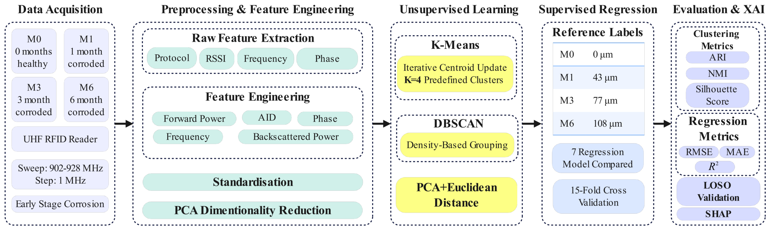
The methodological workflow of this study is shown in Figure 1 and begins with collecting real-time UHF RFID tag readings of different durations, processing the raw data, measuring engineering features, applying clustering algorithms, and evaluating them for early-stage corrosion detection, applying supervised regression algorithms for nominal corrosion-thickness state estimation in the early stages, evaluating the algorithms, and testing the interpretability of the supervised models.

3.1. Dataset Acquisition

The dataset used in this study contains raw UHF RFID tag readouts collected from corrosion-exposed samples over different exposure durations. The corrosion samples consist of mild steel (S275) plates with dimensions of 300 mm × 150 mm × 3 mm, supplied by International Paint Ltd., Newcastle upon Tyne, UK.

The centre region of each plate (30 mm × 30 mm) was exposed to a marine atmosphere for a controlled duration of 0, 1, 3, 6, 10, and 12 months to produce progressive stages of corrosion. Following exposure, the corroded area was sealed with a non-conductive paint layer of approximately 100 μm thickness, as described in the original experimental study [7].

Data were acquired using a ThingMagic Mercury xPRESS RFID reader platform. A circularly polarised reader antenna with a gain of 6 dBi was positioned at a fixed standoff distance of 1 m from the tag. To obtain the threshold forward power required to activate the tag ($P_{in}^{to}$) and the corresponding backscattered power ($P_{R\leftarrow T}$), the reader output was stepped down from 30 dBm in increments of 0.5 dB, yielding a maximum Effective Isotropic Radiated Power (EIRP) of 4 W. The frequency sweep covered 902–928 MHz in 1 MHz steps, and each sample was measured four times to ensure robustness. Measurements were conducted in a typical indoor office environment containing metallic furniture and other sources of multipath clutter [7]. All RFID measurements were acquired under controlled laboratory conditions. During data acquisition, the relative positions of the RFID reader, antenna, and test samples were maintained constant to minimise geometric variability. No intentional metallic or dielectric reflectors were introduced into the reader–tag path. Therefore, the dataset primarily captures variations caused by corrosion progression rather than environmental perturbations [7]. RFID system performance depends on the relative geometry between reader and tag antennas. Variations in alignment can change antenna coupling and polarisation matching, leading to variations in received signal strength and communication reliability. Previous RFID studies have identified polarisation mismatch and geometric orientation as important contributors to RFID link variability [2,7,11]. Also, antenna tilt can alter the polarisation relationship between the reader and RFID tag. RFID link-budget studies have shown that polarisation mismatch introduces additional signal attenuation and may reduce received power levels. Consequently, significant reader antenna tilt may influence feature values used by the classifier [22]. Since the present experiments were conducted using a fixed antenna orientation and reader and sample positioning were maintained constant throughout data acquisition, classification results represent corrosion-induced variability under fixed geometric conditions.

Six data files (M0, M1, M3, M6, M10, and M12) represent samples exposed for 0, 1, 3, 6, 10, and 12 months, respectively. Although the raw dataset includes M10 and M12 samples, this study focuses on early-stage corrosion monitoring using M0, M1, M3, and M6. The later-stage samples were excluded because the objective was early detection and thickness estimation before severe material degradation. The M10 and M12 samples remain part of the original dataset reported in [7]; however, they were intentionally excluded from the present analysis because the focus of this work is early-stage corrosion monitoring. Restricting the analysis to M0, M1, M3, and M6 allows evaluation of whether RFID-derived features can identify and estimate corrosion progression before substantial material degradation occurs. The structured dataset comprises 384, 293, 304, and 108 records for M0, M1, M3, and M6, respectively, yielding 1089 records in total. It should be noted that the 1089 entries in the dataset represent RFID measurement records rather than 1089 independent physical corrosion specimens. Each corrosion-stage file contains multiple RFID reads collected during frequency-sweep measurements, repeated several times for the same underlying specimen. Therefore, the dataset comprises repeated observations of a limited number of physical corrosion samples rather than a collection of fully independent experimental specimens. Consequently, multiple records originate from the same physical specimen under comparable experimental conditions, differing primarily in operating frequency, reader activation conditions, and repeated measurement events [7,23]. The readcount field is the ThingMagic Mercury reader’s cumulative per-tag readcounter: an integer that increments by one each time the reader successfully activates and reads the RFID tag at any frequency and power level, accumulated continuously since the start of the measurement operation, with its value at any given record reflecting how many successful tag read events have occurred up to that point in the measurement sequence. The description of the engineered features is presented in

Table 1. Description of each feature.

Feature Name	Data Type	Description	Physical Significance
Protocol	Categorical	Encodes the reader’s transmission power setting.	A higher protocol value corresponds to higher forward power (dBm).
RSSI	Integer	Represents the received signal strength (in dBm) of the backscattered tag response measured by the reader.	Indicates how strongly the tag’s signal returns to the reader, making it sensitive to tag–reader distance, material condition, and attenuation caused by corrosion.
Frequency	Integer	Carrier frequency (in kHz) at which the tag was read.	Data was collected over a sweep (902–928 MHz) to capture frequency-dependent responses.
Phase	Integer	Average phase angle of the tag response (0–180°).	Sensitive to changes in the signal’s path length and reflective environment.

.

3.2. Raw Dataset Construction and Feature Engineering

A structured dataset was formed from the text data files of different durations (M0, M1, M3, M6), extracting protocol, antenna number, readcount, RSSI value, frequency, and phase. Here, M0 represents healthy samples, and M1, M3, and M6 belong to the early stage of corrosion [7]. The forward power, $P_{in}$, was calculated using the following equations:

$$P_{in,\mathrm{dBm}}=\mathrm{protocol}\times 0.5+10$$

(1)

$$P_{in,\mathrm{mW}}={10}^{P_{in,\mathrm{dBm}}/10}$$

(2)

The RSSI value was considered a reliable proxy for the tag’s backscattered power. Variations in RSSI directly correspond to changes in the backscattering strength caused by corrosion-induced detuning and impedance mismatch computed using the relation [7]:

$$\mathrm{RSSI}\approx P_{R\leftarrow T,\mathrm{dBm}}$$

(3)

$$P_{R\leftarrow T,\mathrm{mW}}={10}^{P_{R\leftarrow T,\mathrm{dBm}}/10}$$

(4)

where $P_{R\leftarrow T,\mathrm{mW}}$ is the backscattered power expressed in dBm and mW, respectively.

The two powers were then combined to measure the Analogue Identifier (AID), where the threshold value, $P_{th}$, was set to $-17.4$ dBm [7]. The AID can be expressed as follows [7]:

$$\begin{array}{cc}\hfill \mathrm{AID}\left[\psi \right]& ={\displaystyle \frac{P_{th}}{\sqrt{P_{in}^{to}\left[\psi (\theta ,\varphi )\right]·P_{R\leftarrow T}\left[\psi (\theta ,\varphi )\right]}}}\hfill \\ \hfill & ={\displaystyle \frac{2R_L}{\left|Z_A\left[\psi \right]+Z_L\right|}}\hfill \end{array}$$

(5)

$$P_{th,\mathrm{mW}}={10}^{-17.4/10}\approx 0.01820\mathrm{mW}$$

(6)

where $P_{th}$ denotes the chip’s fixed activation threshold power (the minimum incident power required to activate the tag chip), $P_{in}^{to}\left[\psi (\theta ,\varphi )\right]$ denotes the threshold forward power required to activate the tag, where $\psi (\theta ,\varphi )$ is the sensing variable representing the combined effect of corrosion state and reader-tag orientation $(\theta ,\varphi )$, $P_{R\leftarrow T}\left[\psi (\theta ,\varphi )\right]$ denotes the corresponding backscattered power, $R_L$ denotes the resistive part of the tag chip impedance $Z_L=R_L+j{X}_L$, and $Z_A\left[\psi \right]=R_A\left[\psi \right]+j{X}_A\left[\psi \right]$ denotes the complex antenna impedance as a function of corrosion state $\psi$.

Both forms of Equation (5) are dimensionless. In the power-ratio form, $P_{th}$, $P_{in}^{to}$, and $P_{R\leftarrow T}$ are all expressed in milliwatts, so the ratio $P_{th}/\sqrt{P_{in}^{to}·P_{R\leftarrow T}}$ is dimensionless, as the numerator and denominator carry identical units that cancel. In the impedance form, both $2R_L$ and $|Z_A\left[\psi \right]+Z_L|$ are in ohms, yielding the same dimensionless result.

Under the assumption of line-of-sight propagation and the Friis transmission formula [7], geometric terms including reader-tag distance, reader and tag antenna gains, wavelength, and polarisation efficiency appear in both $P_{in}^{to}$ and $P_{R\leftarrow T}$. In the power ratio of AID, these terms partially compensate, reducing the sensitivity of AID to reader-tag geometry under ideal measurement conditions. What remains in the ratio is primarily determined by the tag chip impedance $Z_L$ and the antenna impedance $Z_A\left[\psi \right]$, which changes as corrosion alters the electromagnetic properties of the steel substrate. It should be emphasised that the geometric compensation provided by AID is only approximate and is derived under idealised line-of-sight propagation assumptions. In practical corrosion-monitoring environments, additional electromagnetic effects including multipath propagation, polarisation mismatch, metallic edge diffraction, chip nonlinearity, multiple rust layers, and non-uniform oxide growth may introduce coupling losses that are not fully cancelled within the AID formulation. Consequently, AID should be interpreted as a feature with reduced sensitivity to reader-tag geometry rather than complete immunity to geometric and environmental influences. In practice, multipath propagation, polarisation mismatch, chip nonlinearity, edge effects of metallic components, multiple rust layers, and non-uniform oxide growth introduce additional coupling losses not captured by the idealised formulation, defining the boundary conditions under which this geometric compensation holds.

Although both $Z_L=R_L+j{X}_L$ and $Z_A\left[\psi \right]=R_A\left[\psi \right]+j{X}_A\left[\psi \right]$ are complex-valued, the denominator $\left|Z_A\left[\psi \right]+Z_L\right|$ applies the complex modulus, defined as:

$$\left|Z_A\left[\psi \right]+Z_L\right|=\sqrt{{\left(R_A\left[\psi \right]+R_L\right)}^2+{\left(X_A\left[\psi \right]+X_L\right)}^2}$$

(7)

This ensures that $\mathrm{AID}\left[\psi \right]\in {\mathbb{R}}^{+}$ for all corrosion states $\psi$, regardless of the complex-valued nature of $Z_A\left[\psi \right]$ and $Z_L$. The step-by-step computation of AID with units at each stage is summarised in

Table 2. Step-by-step computation of the AID feature with units at each stage.

Step	Quantity	Expression	Unit	Notes
1	Forward power (dBm)	$P_{in,\mathrm{dBm}}^{to}=\mathrm{protocol}\times 0.5+10$	dBm	Protocol field maps to reader output level.
2	Forward power (mW)	$P_{in,\mathrm{mW}}^{to}={10}^{P_{in,\mathrm{dBm}}^{to}/10}$	mW	Linear conversion from dBm.
3	Backscattered power (dBm)	$P_{R\leftarrow T,\mathrm{dBm}}\approx \mathrm{RSSI}$	dBm	RSSI used as proxy for backscattered power.
4	Backscattered power (mW)	$P_{R\leftarrow T,\mathrm{mW}}={10}^{\mathrm{RSSI}/10}$	mW	Linear conversion from dBm.
5	Chip activation threshold	$P_{th,\mathrm{mW}}={10}^{-17.4/10}\approx 0.01820$	mW	Fixed read sensitivity of IMPINJ MONZA 4QT; constant across all samples.
6	AID (power-ratio form)	$\mathrm{AID}\left[\psi \right]={\displaystyle \frac{P_{th,\mathrm{mW}}}{\sqrt{P_{in,\mathrm{mW}}^{to}·P_{R\leftarrow T,\mathrm{mW}}}}}$	Dimensionless	Power ratio partially compensates for orientation and distance effects under ideal conditions; numerator and denominator both in mW.
7	AID (impedance form)	$\mathrm{AID}\left[\psi \right]={\displaystyle \frac{2R_L}{|Z_A\left[\psi \right]+Z_L|}}$	Dimensionless	$|·|$ denotes complex modulus; ensures AID $\in {\mathbb{R}}^{+}$ despite complex $Z_A\left[\psi \right]$, $Z_L$.

.

The features were standardised using standard scaling before being passed to the algorithm. The standardisation was done through the following equation:

$$Z={\displaystyle \frac{x-\mu }{\sigma }}$$

(8)

where x denotes the sample reading, $\mu$ denotes the mean value, and $\sigma$ denotes the standard deviation.

Standardisation is used to rescale all features to a common scale so that no single feature dominates the model, ensuring fair comparison, faster convergence, and better performance. The PCA technique was applied here not only to visualise the separation of the clusters clearly in 2D space but also to remove redundancy between features. RFID features are often correlated, and PCA transforms them into uncorrelated components, which makes clustering algorithms work better.

3.3. Corrosion Detection (Unsupervised Clustering)

Various clustering algorithms, such as K-Means and Density-Based Spatial Clustering of Applications with Noise (DBSCAN), were applied here to determine whether corrosion-stages could be distinguished without labels. In the training process, the algorithms were tested with different combinations of the features such as (forward power, frequency, phase), (frequency, phase, backscattered power), (AID, phase, frequency), (forward power, AID, frequency), etc. to determine the optimal feature combinations that clustering algorithms can use to effectively separate the corrosion-stages.

Here, clustering was used to automatically group RFID tag readings based on how their electromagnetic properties changed during corrosion, without providing any prior labels. Each RFID measurement was represented as a vector of the available features extracted from the tag’s response. Each data point can be written as a vector ${\mathbf{x}}_i$ as follows:

$${\mathbf{x}}_i=\left({\mathrm{AID}}_i,P_{fw,i},f_i,\dots \right),i=1,2,3,\dots$$

(9)

From Equation (9), the complete dataset can be written as $X=\{{\mathbf{x}}_1,{\mathbf{x}}_2,{\mathbf{x}}_3,\dots ,{\mathbf{x}}_n\}$. Here, ${\mathrm{AID}}_i$ denotes an impedance-derived antenna feature, $P_{fw}$ represents the power interaction between the RFID reader and tag, and $f_i$ corresponds to the operating or resonant frequency at which the measurement is taken. These features form a multidimensional feature space, where each axis corresponds to one RFID parameter. The core idea of clustering is that measurements with similar electromagnetic behaviour (for example, similar impedance or backscatter response due to similar corrosion states) will lie close together in this space, while those with different corrosion characteristics will be farther apart. To measure how close or far apart two RFID readings are, the Euclidean distance metric is calculated as follows:

$$d({\mathbf{x}}_i,{\mathbf{x}}_j)=\sqrt{{({\mathrm{AID}}_i-{\mathrm{AID}}_j)}^2+{(P_{fw,i}-P_{fw,j})}^2+{(f_i-f_j)}^2+\dots }$$

(10)

If this distance is small, both readings have nearly the same tag impedance and power interaction pattern, indicating a similar corrosion condition.

K-Means: In the K-Means algorithm, the number of clusters has to be predefined by the user. It begins with k initial centres (means) $({\mu }_1,{\mu }_2,\dots ,{\mu }_k)$ and then repeats two main steps:

Assignment Step: Each RFID reading ${\mathbf{x}}_i$ is assigned to the cluster whose centre is closest to it:

$$r_{ij}=1\mathrm{if}j=arg\underset{l}{min}d({\mathbf{x}}_i,{\mu }_l)$$

(11)

Update Step: Each cluster centre is recalculated as the average of all readings in that group:

$${\mu }_j={\displaystyle \frac{{\sum }_i{r}_{ij}{\mathbf{x}}_i}{{\sum }_i{r}_{ij}}}$$

(12)

Through this iterative refinement, K-Means groups RFID readings with similar electromagnetic responses, such as similar AID, $P_{fw}$, and f values, which correspond to specific corrosion-stages (i.e., M0, M1, M3, M6).

DBSCAN: This algorithm groups RFID readings based on how densely they are packed in the feature space, rather than by distance to a centre.

Each reading ${\mathbf{x}}_i$ checks its nearby readings within a certain distance threshold ($\epsilon$). This neighbourhood is defined as:

$$N_{\epsilon }\left({\mathbf{x}}_i\right)=\{{\mathbf{x}}_j\in X\mid d({\mathbf{x}}_i,{\mathbf{x}}_j)\le \epsilon \}$$

(13)

If a reading has several neighbours greater than or equal to a minimum value (minPts), it is called a core point:

$$|N_{\epsilon }\left({\mathbf{x}}_i\right)| \ge \mathit{minPts}$$

(14)

Readings that are within the neighbourhood of a core point are grouped together, and this grouping process continues recursively, connecting all nearby points that share dense regions. Mathematically, the resulting cluster $C_m$ contains all points that are density-connected to at least one core point:

$$C_m=\{{\mathbf{x}}_i\mid {\mathbf{x}}_i\mathrm{is}\text{density-connected}\mathrm{to}\mathrm{a}\mathrm{core}\mathrm{point}{\mathbf{x}}_c\}$$

(15)

Points that do not belong to any dense region are treated as isolated noise, often caused by unstable or irregular RFID readings.

3.4. Nominal Corrosion-Thickness State Estimation (Supervised Regression)

An early study measured the average value of corrosion layer thickness for 1, 3, and 6 months with laser profilometry, where the exposed corrosion samples were found to be 43 μm, 77 μm, and 108 μm [7]. These thickness values represent average nominal corrosion-product thicknesses obtained from laser profilometry measurements reported by Zhang et al. [7]. Because early corrosion is characterised by localised pitting and spatially non-uniform corrosion-product growth, these values are interpreted as nominal average corrosion states used for regression modelling. Following that study, the corrosion samples of M0, M1, M3, and M6 were labelled with 0 μm, 43 μm, 77 μm, and 108 μm. Then, different traditional regression models were trained here, including Ridge, Lasso, ElasticNet, DecisionTree, Random Forest, GradientBoosting, and AdaBoost Regressor.

3.5. Algorithm Evaluation

The clustering algorithms were evaluated using Adjusted Rand Index (ARI), Normalised Mutual Information (NMI), and Silhouette Coefficient. The higher the value of these metrics, the closer to one, the better the cluster formation of distinct corrosion stages will be.

The regression models were evaluated using the Root Mean Squared Error (RMSE), Mean Absolute Error (MAE), and R-squared ($R^2$) score.

3.6. Explainable AI

The interpretability of the best-performing supervised regression model was tested using the Shapley Additive exPlanations (SHAP) technique. It is a technique from cooperative game theory used to explain how much each feature contributes to a model’s prediction. In this study, SHAP values quantify how strongly each RFID parameter influences the predicted nominal corrosion-thickness state. A positive SHAP value of a feature represents that the feature pushes the prediction of the model towards higher corrosion thickness. A negative SHAP value of a feature means that the feature pushes the prediction towards lower corrosion thickness.

4. Result Analysis

This section presents and discusses the results obtained using the methodology described in Section 3, focusing on the capability of RFID-derived electromagnetic features to characterise and quantify corrosion progression. Initially, key features—Analogue identifier (AID), forward power, backscattered power, phase, and frequency—were analysed across four corrosion-stages (M0, M1, M3, and M6) to assess their sensitivity to degradation. The results indicate that AID and forward power exhibit clear and consistent shifts with increasing corrosion severity, particularly at early stages, whereas phase and backscattered power show weaker or noisier trends. Building on these observations, unsupervised clustering techniques (K-Means and DBSCAN) combined with PCA were employed to evaluate the separability of corrosion stages using different feature combinations, followed by supervised regression models to estimate nominal corrosion-thickness state. Finally, explainable AI techniques were applied to validate the physical relevance of the most influential features, linking the data-driven results to underlying electromagnetic behaviour.

4.1. Corrosion Progression Based on Multiple Features

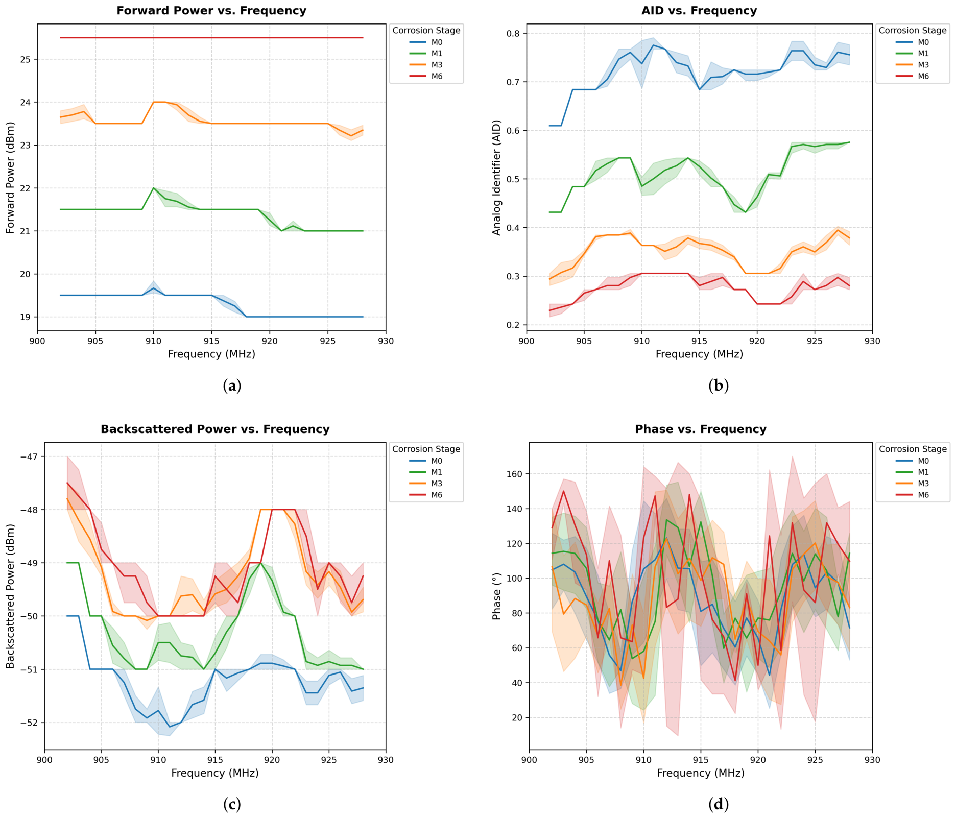
The features (i.e., AID, forward power, backscattered power, phase, and frequency) were first analysed to understand their behaviour across different corrosion-stages (i.e., M0, M1, M3, and M6). Figure 2 shows that AID and forward power exhibited a clear and consistent shift between the healthy stage (M0) and the early corrosion stages (M1, M3, M6) with respect to frequency, making them the most promising indicators of corrosion progression. As depicted in Figure 2a, forward power demonstrates the strongest discriminatory capability. The healthy stage (M0) requires the lowest forward power, fluctuating smoothly between 19 and 19.5 dBm. Subtle dips in these curves indicate optimal frequencies where the antenna impedance is best matched, thereby minimising the required activation power (e.g., between 920 and 930 MHz for M0). As corrosion progresses, the required forward power increases substantially, culminating in the M6 stage, which exhibits a stable, flat response at approximately 25.5 dBm across the entire frequency sweep. This observation confirms that the magnitude of the forward power is a much stronger indicator of corrosion severity than the operating frequency.

Similarly, Figure 2b illustrates that the Analogue Identifier (AID) inversely correlates with corrosion progression. M0 exhibits the highest AID values, fluctuating between 0.6 and 0.8, while the more severely corroded M6 stage drops to values between 0.2 and 0.3. Despite frequency-dependent fluctuations, the distinct stratification between stages remains clear.

Conversely, backscattered power (Figure 2c) and phase (Figure 2d) display significant overlap and high variance across the frequency band. While backscattered power shows some general separation between M0 and the corroded states, stages M3 and M6 overlap heavily (fluctuating between $-51$ and $-47$ dBm). The phase response is highly erratic for all stages, rendering it an unreliable feature for isolated stage discrimination. The observed corrosion response is not strictly linear. Corrosion progression alters not only the thickness of the oxide layer but also its dielectric properties, surface roughness, permeability, conductivity, and spatial uniformity. These factors influence the RFID antenna impedance through complex electromagnetic interactions that may vary across the corroded region. Consequently, fluctuations in AID and forward power are expected even within the same nominal corrosion stage, particularly during the transition from healthy to early-stage corrosion. The physical basis of RFID corrosion sensing arises from the interaction between the tag antenna electromagnetic field and the corroding metallic substrate. As corrosion develops, the local conductivity, magnetic permeability, surface roughness, and corrosion-product morphology of the steel surface change [7,10,24]. These changes modify the antenna boundary conditions, impedance matching, coupling efficiency, and backscatter response of the RFID tag [25]. Previous LF RFID corrosion studies have similarly shown that conductivity and permeability variations in corrosion layers influence RFID impedance matching and sensing performance [10,24]. Therefore, variations in RFID-derived features are not purely empirical but originate from corrosion-induced changes in the electromagnetic interaction between the tag antenna and the steel substrate. RFID measurements are inherently influenced by the surrounding electromagnetic environment. Previous RFID propagation studies have shown that nearby conductive or dielectric objects can introduce multipath scattering, reflection, and blockage effects that alter received signal strength and backscatter performance [26]. Although no controlled reflector experiments were performed in this study, evaluating classifier robustness under deliberately introduced metallic or dielectric reflectors represents an important direction for future work. The present work intentionally focused on establishing the feasibility of corrosion detection under controlled laboratory conditions by minimising environmental variability.

To assess the capability of different features in distinguishing corrosion stages, both K-Means and DBSCAN clustering algorithms were tested on multiple feature combinations. PCA was applied to reduce dimensionality while preserving the maximum variance in the data.

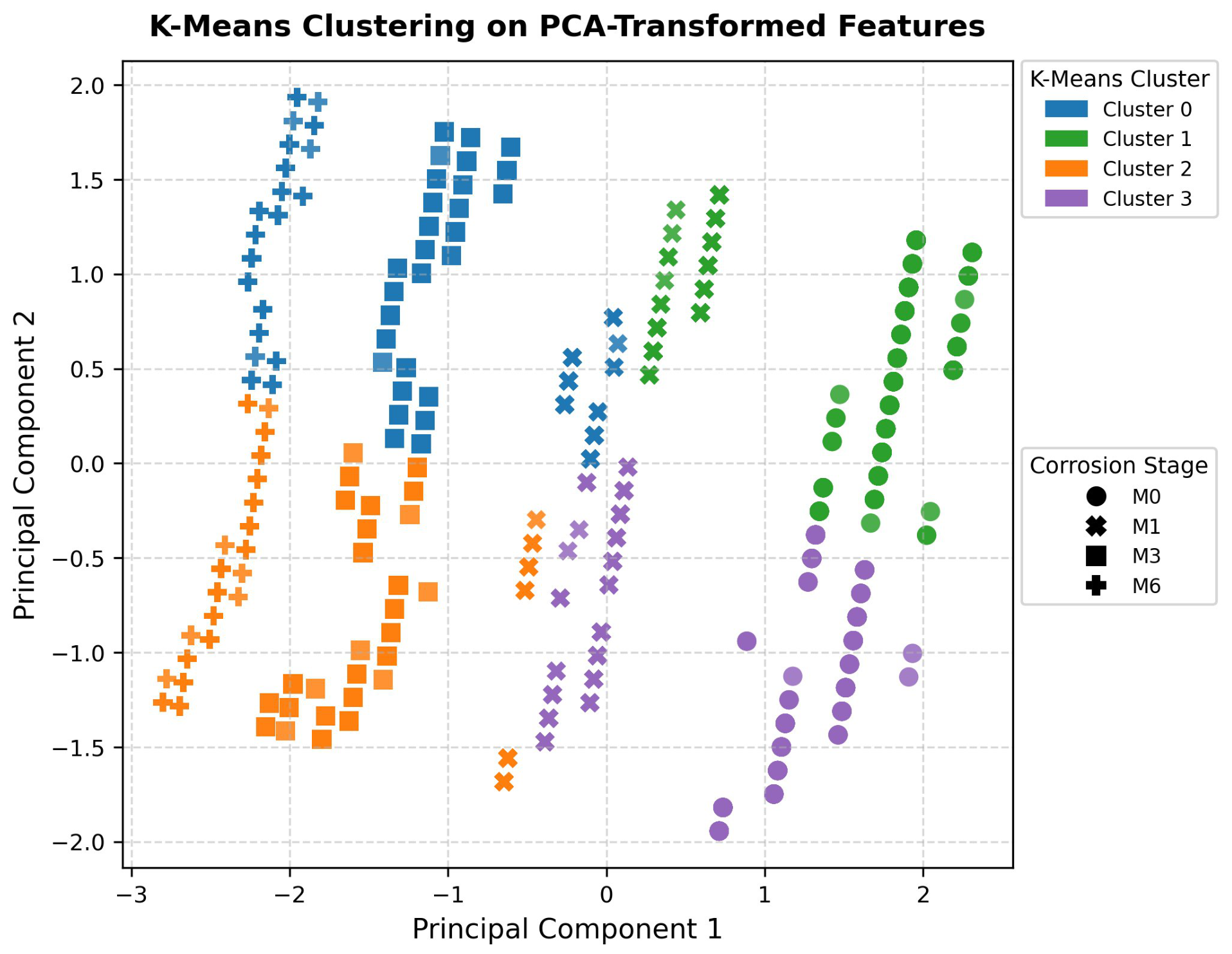
K-Means achieved its best performance with the feature set (AID, Forward Power, Frequency), yielding an ARI = 0.332, NMI = 0.459, and a Silhouette score = 0.434. Across all tested feature combinations, ARI values ranged from 0.195 to 0.332, indicating that K-Means consistently fails to separate the corrosion stages. This behaviour is attributed to the gradual and non-linear shift in RFID features caused by surface impedance variations, which the centroid-based structure of K-Means cannot adequately capture.

Table 3. Experimental results of the K-Means clustering with PCA-transformed different combinations of feature sets.

Feature Set	ARI	NMI	Silhouette
Forward power, AID, frequency	0.332	0.459	0.434
Forward power, backscattered power, frequency	0.288	0.399	0.404
AID, forward power, backscattered power, phase, frequency	0.285	0.394	0.262
AID, frequency	0.272	0.378	0.458
Forward power, backscattered power, phase, frequency	0.252	0.348	0.276
AID, phase, frequency	0.211	0.307	0.295
Forward power, phase, frequency	0.195	0.312	0.291

summarises the experimental outcomes for all tested K-Means feature combinations.

As shown in Figure 3, K-Means produced four predefined clusters, but with partial overlap between adjacent groups.

The cluster corresponding to the M1 stage partially overlapped with the M0 stage, and similarly, the cluster corresponding to the M3 stage overlapped with the cluster of the M6 stage, confirming that the K-Means algorithm struggles with the non-linear and density-varying structure of the RFID feature space.

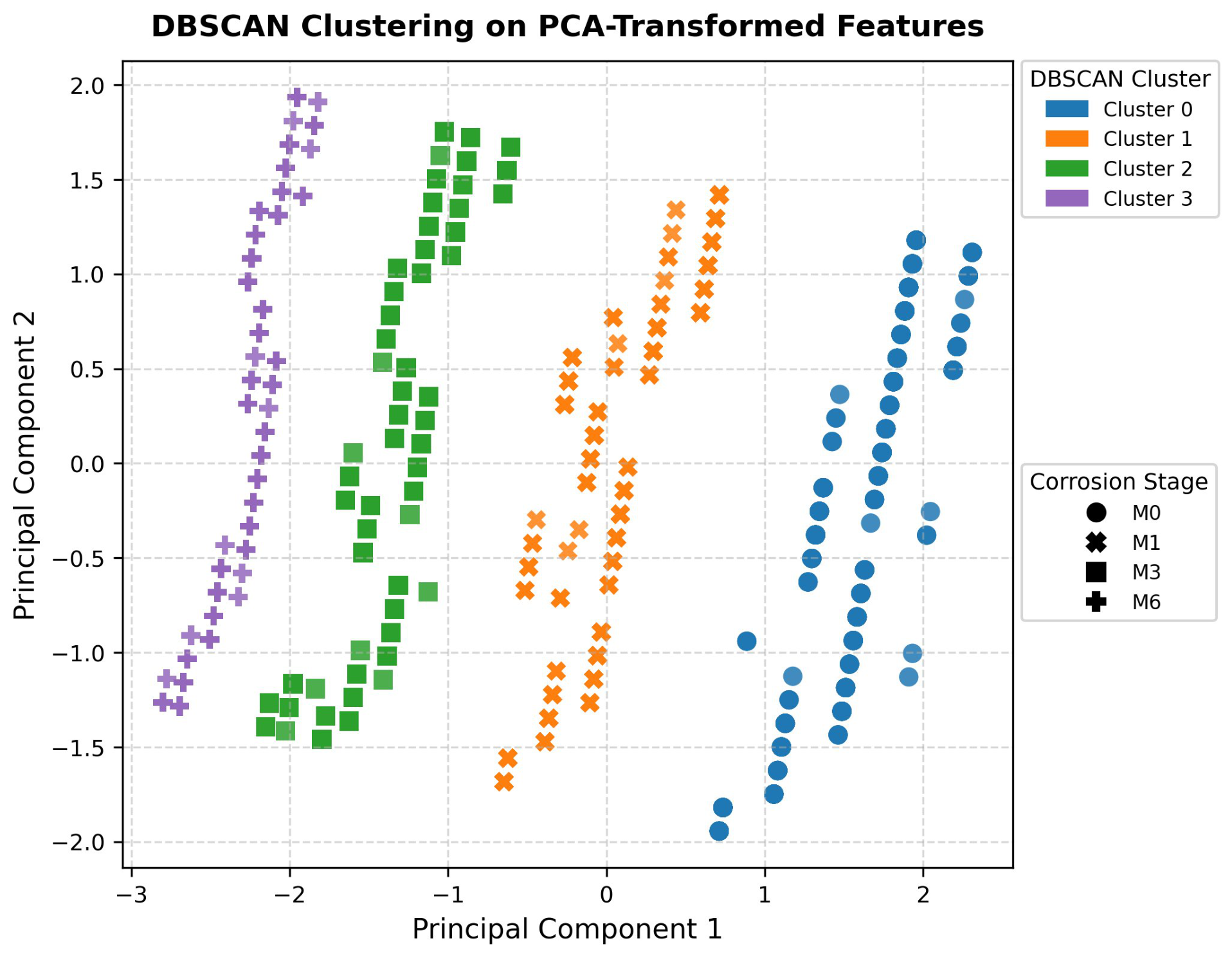
DBSCAN identified four distinct clusters that aligned with the four nominal corrosion stages within the analysed dataset. This suggests that the corrosion stages present in the available dataset exhibit strong separability within the selected feature space.

Table 4. Experimental top results of the DBSCAN clustering with PCA-transformed different combinations of feature sets with different values of eps and min samples.

Features	eps	Min Samples	ARI	NMI	Silhouette	Clusters Found	Noise Points
Forward power, AID, frequency	0.5	5	1	1	0.790	4	0
Forward power, AID, frequency	0.6	4	1	1	0.327	4	0
Forward power, AID, frequency	0.6	5	1	1	0.327	4	0
Forward power, frequency	0.3	3	1	1	0.264	4	0
Forward power, phase, frequency	0.5	5	0.991	0.975	0.05	6	1
Forward power, backscattered power, frequency	0.5	3	0.409	0.639	0.479	26	3
AID, forward power, backscattered power, phase, frequency	0.6	4	0.401	0.617	0.158	29	34

summarises the experimental outcomes for all tested DBSCAN parameter combinations.

As shown in Figure 4, the DBSCAN algorithm generated four well-separated individual clusters by identifying similar patterns in the data without defining the number of clusters required.

The clusters are correctly aligned with the ground truth of corrosion-stages (ARI = 1.000, NMI = 1.000, Silhouette = 0.790, as shown in Table 4). DBSCAN was trained without using corrosion-stage labels; labels were used only for post hoc evaluation through ARI and NMI, highlighting the potential of density-based clustering for corrosion-stage separation in UHF RFID data under the tested conditions.

4.2. Nominal Corrosion-Thickness State Estimation (Supervised Regression)

Different traditional regression models were trained and evaluated to estimate nominal corrosion-thickness state. The nominal corrosion-thickness labels (0, 43, 77, and 108 μm) were assigned to stages M0, M1, M3, and M6, respectively, based on direct laser profilometry measurements reported in a prior study [7]. Two complementary validation strategies were employed: a standard 90:10 train/test split with 15-fold cross-validation to assess the overall model stability, and Leave-One-Sample-Out (LOSO) validation defined at the readcount level to evaluate generalisation across repeated measurement sessions from the same physical specimens.

4.2.1. 15-Fold Cross-Validation

All models were first trained and validated through 15-fold cross-validation using a 90:10 training-to-testing ratio (as shown in

Table 5. Evaluation metrics of the regression models with 15-fold cross-validation.

Model	RMSE	MAE	R2
Ridge Regressor	$9.74\pm 0.54$	$8.34\pm 0.49$	$0.93\pm 0.01$
Lasso	$11.27\pm 0.91$	$9.19\pm 0.72$	$0.91\pm 0.01$
Elastic Net	$35.49\pm 2.06$	$30.13\pm 2.57$	$0.08\pm 0.02$
DecisionTree	$1.49\pm 2.17$	$0.21\pm 0.35$	$0.99\pm 0.01$
Random Forest	$1.34\pm 1.31$	$0.21\pm 0.24$	$1.00\pm 0.00$
GradientBoosting	$2.16\pm 0.87$	$0.97\pm 0.28$	$1.00\pm 0.00$
AdaBoost	$4.91\pm 0.68$	$1.84\pm 0.45$	$0.98\pm 0.00$

). ElasticNet performed very poorly ($R^2\approx 0.08$) and essentially failed to predict the thickness of the layers. Ridge and Lasso showed moderate performance ($R^2\approx 0.91$–$0.93$), but with high errors, not suitable for precise nominal corrosion-thickness state estimation. Decision Tree had good accuracy ($R^2\approx 0.99$), but the high standard deviation of RMSE ($\pm 2.17$) shows it is unstable and prone to overfitting. Gradient Boosting and AdaBoost showed a higher $R^2$ score, but with slightly higher errors than Random Forest. Random Forest achieved the lowest errors (RMSE = 1.34 μm, MAE = 0.21 μm) and an $R^2$ of 1.00 with very small variance, making it the most reliable model under this validation strategy. It should be noted that the regression analysis presented in this study is based on four experimentally measured nominal corrosion-thickness values (0, 43, 77, and 108 µm) obtained from the original corrosion characterisation study [7]. Consequently, the reported regression performance should be interpreted as an accurate estimation of nominal corrosion-thickness state within the available label space rather than unrestricted prediction across a continuous corrosion-thickness spectrum. Although the model outputs continuous numerical values, validating its predictive capability beyond the experimentally observed thickness levels remains an important next step for future research, which can be achieved using datasets containing additional independently measured corrosion thicknesses.

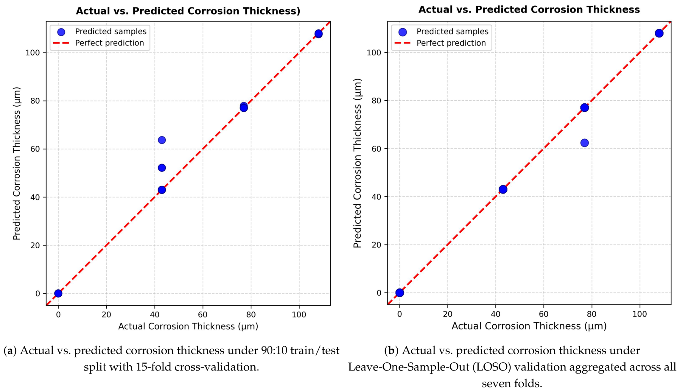
The performance of the Random Forest model was further examined using the held-out test samples from the 90:10 split. As shown in Figure 5a, most test samples were predicted close to the identity line; however, several samples associated with the nominal 43 µm corrosion-stage (M1) exhibited larger prediction deviations than the other corrosion-stages. This behaviour is physically consistent with the characteristics of very early-stage corrosion. At this stage, corrosion products are typically thin, spatially heterogeneous, and strongly influenced by local variations in oxide-layer dielectric constant, surface roughness, conductivity, permeability, and corrosion morphology. Localised pitting and non-uniform oxide growth can generate spatially varying impedance distributions across the sensing region, producing non-linear fluctuations in the RFID response that are not completely represented by the aggregate AID and forward-power features. Consequently, the M1 stage exhibits greater electromagnetic variability and prediction uncertainty than the more developed corrosion stages. As noted by Zhang et al. [7], surface roughness, conductivity, and permeability of the corroded area all contribute to antenna impedance variation, producing non-linear and spatially heterogeneous electromagnetic coupling effects that are not fully captured by the aggregate AID and forward power features at this early stage. All other thickness values were accurately predicted by the model.

4.2.2. Leave-One-Sample-Out (LOSO) Validation

To further validate the robustness of the regression results and assess generalisation across distinct subsets of the dataset, a Leave-One-Sample-Out (LOSO) validation strategy was applied using the readcount value as the grouping variable. The readcount field is the ThingMagic Mercury reader’s cumulative per-tag readcounter, recording how many successful tag activation events have accumulated since the start of the measurement operation. The LOSO validation therefore operates at the measurement-event level, grouping records by their cumulative read event number across the dataset. This counter naturally produces different value ranges across corrosion stages: less-corroded samples (M0, M1, M3) activate readily from the earliest reads and contribute records across readcount values 1–6, whereas the most-corroded sample (M6) only activates after the reader has accumulated many reads from lower-threshold samples, producing records exclusively at readcount values 5–7. The combined dataset yields seven unique readcount values (1 through 7). In each LOSO fold, all records sharing one unique readcount value were held out entirely as the test set, while the remaining records were used for training. The feature scaler was fitted exclusively on the training data in each fold to prevent preprocessing leakage. A fresh model instance was initialised and fitted independently within each fold to ensure no model state carried over between folds. The term “sample” in the LOSO procedure refers to a measurement-event grouping based on the readcount variable rather than an independent physical corrosion specimen. Accordingly, LOSO validation in this study evaluates generalisation across repeated measurement events while reducing within-session data leakage. The fold construction, including test set size and per-stage record counts, is reported in

Table 6. LOSO fold construction: left-out readcount, test set size, per-stage record distribution, and training set size across all seven folds.

Fold	Left-Out Readcount	Test Records	M0	M1	M3	M6	Train Records
1	1	34	7	8	19	0	1055
2	2	41	12	16	13	0	1048
3	3	40	10	17	13	0	1049
4	4	120	50	55	15	0	969
5	5	526	232	152	103	39	563
6	6	320	73	44	136	67	769
7	7	8	0	1	5	2	1081

.

Table 7. Evaluation metrics of the regression models with Leave-One-Sample-Out (LOSO) validation (Mean ± Std across 7 folds).

Model	RMSE	MAE	R2
Ridge Regressor	$4.27\pm 0.65$	$3.72\pm 0.68$	$0.98\pm 0.01$
Lasso	$4.57\pm 1.14$	$3.85\pm 1.03$	$0.97\pm 0.01$
Elastic Net	$9.46\pm 1.40$	$8.25\pm 0.99$	$0.88\pm 0.09$
DecisionTree	$0.27\pm 0.67$	$0.02\pm 0.04$	$1.00\pm 0.00$
Random Forest	$0.12\pm 0.29$	$0.01\pm 0.02$	$1.00\pm 0.00$
GradientBoosting	$0.14\pm 0.35$	$0.01\pm 0.02$	$1.00\pm 0.00$
AdaBoost	$0.27\pm 0.67$	$0.02\pm 0.04$	$1.00\pm 0.00$

reports the mean and standard deviation of RMSE, MAE, and $R^2$ across all seven folds.

The fold-by-fold breakdown reveals an important structural property of this validation. Six of the seven folds (readcounts 1, 2, 3, 4, 5, and 7) yield a Random Forest RMSE of 0.000 μm. Inspection of Table 6 explains why: folds 1 through 4 contain no M6 records in the test set, since M6 only activates at higher cumulative readcount values; these folds therefore test prediction across only three of the four corrosion stages. Fold 7 holds out only 8 records. Among the two folds that contain all four corrosion stages in the test set, fold 6 is the only fold that contains all four corrosion stages in the test set (M0: 73, M1: 44, M3: 136, M6: 67 records) and is the sole source of non-zero prediction error, yielding a Random Forest RMSE of 0.817 μm. The reported mean RMSE of 0.12 μm across all seven folds is therefore dominated by this single fold, and fold 6 represents the most meaningful validation scenario in this dataset. The Random Forest RMSE of 0.817 μm in fold 6 indicates strong predictive consistency of all four thickness classes under this more demanding condition. Linear models (Ridge, Lasso, ElasticNet) showed substantially higher errors across all folds, reflecting their inability to capture the non-linear relationship between RFID features and corrosion thickness. The consistent superiority of Random Forest across both validation strategies confirms it as the most reliable model for nominal corrosion-thickness state estimation in this study. Figure 5b shows the actual versus predicted thickness under LOSO validation, where predictions from all seven folds are aggregated. The results closely follow the identity line, further validating the generalisation across repeated measurement sessions capability of the Random Forest model.

4.3. Corrosion Validation Through Explainable AI

To validate the physical relevance of the features used by the best-performing regression model, the Shapley Additive exPlanations (SHAP) technique was applied to the Random Forest regressor. SHAP values quantify the contribution of each input feature to the model’s prediction. A positive SHAP value indicates that the feature pushes the prediction towards higher corrosion thickness, while a negative SHAP value indicates a push towards lower thickness.

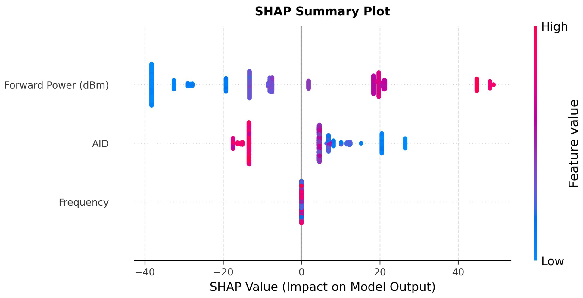
Figure 6 presents the SHAP summary plot, which ranks the three input features by their mean absolute SHAP value across all test samples from the LOSO validation folds. The results reveal a clear hierarchy of feature importance.

Forward power emerged as the most influential feature (Mean |SHAP| = 24.34), with high feature values producing large positive SHAP contributions and low feature values producing large negative contributions. This is physically consistent with the sensing mechanism of RFID-based corrosion monitoring. As corrosion progresses, the growing oxide layer alters the coupling efficiency between the RFID reader and the tag antenna, directly modifying the forward power required to activate the tag. Higher forward power is associated with greater impedance mismatch caused by advanced corrosion, linking it directly to thicker corrosion layers. Forward power is physically meaningful because it represents the reader power required to activate the RFID tag. Corrosion-induced changes in conductivity, permeability, and surface morphology modify the tag antenna impedance and coupling conditions. This alters the power-transfer efficiency between the reader and tag, meaning that more severely corroded samples may require higher activation power. Therefore, the high importance assigned to forward power is consistent with RFID link-budget theory [26], where impedance mismatch and antenna coupling directly affect delivered tag power and read performance.

AID was the second most important feature (Mean |SHAP| = 12.23), with both positive and negative contributions observed across the corrosion stages. AID directly encodes the antenna impedance difference as a function of corrosion progression $\psi$, as defined in Equation (5). As corrosion develops, the surface conductivity and permeability of the steel substrate change, which alters the antenna impedance $Z_A\left[\psi \right]$. This impedance shift directly modifies the AID value, making it a physically meaningful and sensitive indicator of corrosion severity.

Frequency contributed negligible predictive information (Mean |SHAP| = 0.000) to the Random Forest model. This result is explained by the data collection protocol. The same frequency sweep (902 to 928 MHz) was applied identically across all four corrosion-stages (M0, M1, M3, and M6). Consequently, any given frequency value corresponds equally to all corrosion stages and all thickness labels, providing no discriminative information for thickness prediction. The model therefore assigned zero importance to frequency, as it carries no corrosion-specific signal. It is the response of the tag at a given frequency, captured through forward power and AID, which changes with corrosion progression, rather than the frequency sweep itself. This zero contribution reflects a limitation of the fixed frequency sweep design inherited from the original experimental protocol rather than a general physical conclusion. This is consistent with the original experimental design of Zhang et al. [7], who noted that the PCA method extracts shape information from the AID frequency sweep rather than individual frequency values, enabling sensitivity maximisation within the fixed 902–928 MHz measurement band. In systems employing variable frequency scanning or multi-resonant RFID tags, corrosion-induced resonant frequency shifts would be expected to carry discriminative information and may emerge as an important predictive feature. This is further supported by related sweep-frequency corrosion NDT research. Zhang et al. [27] demonstrated in K-band sweep-frequency microwave NDT that selecting individual frequency points for corrosion characterisation is suboptimal, and that the aggregate response across the full frequency sweep carries the dominant diagnostic information. In the UHF RFID context, AID encodes this aggregate sweep response through the power ratio, which is consistent with frequency contributing negligible individual discriminative information while AID emerges as the primary corrosion-sensitive feature.

The SHAP analysis confirms that forward power and AID are the physically dominant features in the Random Forest model’s decision-making, directly linked to impedance changes and resonant frequency shifts induced by corrosion progression. These results reinforce the earlier feature analysis (Figure 2), where the same two features exhibited the clearest sensitivity to corrosion severity across all four stages.

5. Discussion

The findings of this study demonstrate the feasibility of utilising machine learning to interpret complex UHF RFID signals for early-stage corrosion monitoring. A fundamental challenge in RFID-based sensing is the non-linear and noisy nature of the electromagnetic response as corrosion progresses. The clustering results highlight this clearly: K-Means struggled to separate the corrosion stages because it assumes spherical, centroid-based distributions. In contrast, DBSCAN successfully identified four distinct stages (ARI = 1.0) without prior labelling, indicating that early-stage corrosion signatures naturally form density-based clusters in the feature space rather than linear geometric groupings.

The supervised regression analysis further reinforced the non-linear relationship between RFID parameters and corrosion layer thickness. Linear models (ElasticNet, Ridge, Lasso) exhibited poor predictive accuracy, whereas the Random Forest Regressor achieved exceptional performance (RMSE = 1.34 µm under 15-fold cross-validation). Crucially, the Leave-One-Sample-Out (LOSO) validation at the readcount session level (RMSE = 0.12 µm) provided strong evidence that the model learned genuine corrosion-related electromagnetic trends rather than simply memorising within-session artefacts.

The SHAP analysis successfully bridged the gap between data-driven machine learning and electromagnetic physics. By identifying forward power and AID as the dominant predictive features, the model’s decision-making process aligns directly with RFID link-budget theory. As the corrosion layer alters the surface conductivity and permeability of the steel, it shifts the antenna impedance. This mismatch directly impacts coupling efficiency, necessitating higher forward power for tag activation, a physical reality accurately captured by the model. Furthermore, the negligible contribution of frequency in this specific dataset highlights that fixed-frequency sweeps provide diagnostic value primarily through the aggregate power and impedance response, rather than individual frequency data points.

Despite these promising outcomes, several limitations must be acknowledged. The work was conducted under controlled laboratory conditions, and real-world factors such as humidity, temperature variation, electromagnetic interference, and material diversity were not included. Additionally, the absence of a blank non-corroded reference plate under identical environmental conditions means that corrosion-induced signal changes cannot be fully isolated from environmental noise contributions, a constraint inherited from the original experimental protocol [7]. The dataset comprises a small label space of four experimentally measured nominal corrosion-thickness values (0, 43, 77, and 108 µm) derived from a single physical plate per corrosion stage. Therefore, the reported performance should be interpreted as the estimation of nominal corrosion-thickness states within the available experimental range, not as proof of generalised continuous-thickness prediction across varied structural geometries. Validation using independent steel plates, varied corrosion morphologies, and uncontrolled environmental conditions is required before deployment-level generalisation can be claimed. Furthermore, the idealised AID formulation provides partial, rather than absolute, compensation for reader-tag orientation and distance effects. Practical factors such as multipath propagation, edge diffraction, and oxide-layer inhomogeneity may introduce additional coupling effects not explicitly modelled here.

Future research will focus on collecting large-scale, real-time RFID data from operational environments and incorporating environmental variability into the model. Applying advanced deep learning architectures, such as convolutional neural networks, recurrent neural networks, or Transformer-based models, could improve feature learning and temporal corrosion tracking. Further exploration will also involve developing edge-optimised ML models for deployment on resource-constrained RFID hardware and extending the approach to multi-degradation monitoring, such as corrosion-fatigue interaction.

6. Conclusions

This study effectively addressed key gaps in the existing literature by providing a solid analytical foundation for transforming low-cost, passive UHF RFID tags into reliable, distributed sensor networks. Specifically, the key achievements include:

• Introducing a dedicated ML-based solution for corrosion monitoring and material loss estimation using RFID data, bridging the gap between passive electromagnetic sensing and data-driven structural health evaluation.
• Demonstrating unsupervised corrosion-stage detection without relying on labelled datasets. The density-based clustering (DBSCAN) perfectly separated distinct early-stage corrosion phases (ARI = 1.0, NMI = 1.0).
• Establishing a quantitative, interpretable model for nominal corrosion-thickness state estimation with high precision. Validated through both 15-fold cross-validation and LOSO validation at the measurement-session level, the Random Forest Regressor achieved an RMSE of 0.12 µm and an $R^2$ of 1.00.

As an initial feasibility study, these results are based on repeated measurements from a single physical specimen per corrosion stage rather than independent samples. Consequently, while broader multi-specimen experimental validation is the natural next step, this study demonstrates the computational feasibility of using machine learning to decouple genuine corrosion signatures from signal noise, enabling autonomous and highly sensitive structural health monitoring.

References

1. Pekgor, M.; Arablouei, R.; Nikzad, M.; Masood, S. Displacement Estimation via 3D-printed RFID sensors for structural health monitoring: Leveraging machine learning and photoluminescence to overcome data gaps. Sensors 2024, 24, 1233. [Google Scholar] [CrossRef]
2. Zhao, A.; Sunny, A.I.; Li, L.; Wang, T. Machine learning-based structural health monitoring using RFID for harsh environmental conditions. Electronics 2022, 11, 1740. [Google Scholar] [CrossRef]
3. Le, M.; Pham, P.H.; Hoang, S.P.; Le, D.M.; Pham, Q.V.; Luong, V.S. Enhancing corrosion detection in pulsed eddy current testing systems through autoencoder-based unsupervised learning. NDT E Int. 2024, 146, 103175. [Google Scholar] [CrossRef]
4. Xue, C.; Zhang, Y.; Ding, S.; Song, C.; Wang, Y. Comparison research on characterization and evaluation approaches for paint coated corrosion using eddy current pulsed thermography. Sensors 2023, 23, 6889. [Google Scholar] [CrossRef] [PubMed]
5. Fan, M.; Wang, Q.; Cao, B.; Ye, B.; Sunny, A.I.; Tian, G. Frequency optimization for enhancement of surface defect classification using the eddy current technique. Sensors 2016, 16, 649. [Google Scholar] [CrossRef] [PubMed]
6. Benintendi, D.; Tennant, K.M.; Sabolsky, E.M.; Wilhelm, J. Wireless Patch Antenna Characterization for Live Health Monitoring Using Machine Learning. Sensors 2025, 25, 4654. [Google Scholar] [CrossRef] [PubMed]
7. Zhang, J.; Tian, G.Y. UHF RFID tag antenna-based sensing for corrosion detection & characterization using principal component analysis. IEEE Trans. Antennas Propag. 2016, 64, 4405–4414. [Google Scholar] [CrossRef]
8. Zhang, J.; Sunny, A.I.; Zhang, G.; Tian, G. Feature extraction for robust crack monitoring using passive wireless RFID antenna sensors. IEEE Sens. J. 2018, 18, 6273–6280. [Google Scholar] [CrossRef]
9. Sunny, A.I.; Zhang, J.; Tian, G.Y.; Tang, C.; Rafique, W.; Zhao, A.; Fan, M. Temperature independent defect monitoring using passive wireless RFID sensing system. IEEE Sens. J. 2018, 19, 1525–1532. [Google Scholar] [CrossRef]
10. Sunny, A.I.; Tian, G.Y.; Zhang, J.; Pal, M. Low frequency (LF) RFID sensors and selective transient feature extraction for corrosion characterisation. Sens. Actuators A Phys. 2016, 241, 34–43. [Google Scholar] [CrossRef]
11. Zhang, J.; Tian, G.Y.; Marindra, A.M.; Sunny, A.I.; Zhao, A.B. A review of passive RFID tag antenna-based sensors and systems for structural health monitoring applications. Sensors 2017, 17, 265. [Google Scholar] [CrossRef] [PubMed]
12. Sunny, A.I.; Zhao, A.; Li, L.; Sakiliba, S.K. Low-cost IoT-based sensor system: A case study on harsh environmental monitoring. Sensors 2020, 21, 214. [Google Scholar] [CrossRef] [PubMed]
13. Imam, A.; Tian, G.Y. Enhanced sensitivity of low frequency (LF) RFID sensor signal for structural health monitoring (SHM) in high temperature environment. In Proceedings of the 19 World Conference on Non-Destructive Testing, Munich, Germany, 13–17 June 2016; pp. 13–17. [Google Scholar]
14. Tang, C.; Rashvand, H.F.; Tian, G.Y.; Hu, P.; Sunny, A.I.; Wang, H. Structural Health Monitoring with WSNs. In Wireless Sensor Systems for Extreme Environments: Space, Underwater, Underground and Industrial; John Wiley & Sons Ltd: Hoboken, NJ, USA, 2017; pp. 381–408. [Google Scholar]
15. Imran, M.M.H.; Jamaludin, S.; Ayob, A.F.M.; Ali, A.A.I.M.; Ahmad, S.Z.A.S.; Akhbar, M.F.A.; Suhrab, M.I.R.; Zainal, N.; Norzeli, S.M.; Mohamed, S.B. Application of artificial intelligence in marine corrosion prediction and detection. J. Mar. Sci. Eng. 2023, 11, 256. [Google Scholar] [CrossRef]
16. Bouzaffour, K.; Lescop, B.; Talbot, P.; Gallée, F.; Rioual, S. Development of an embedded UHF-RFID corrosion sensor for monitoring corrosion of steel in concrete. IEEE Sens. J. 2021, 21, 12306–12312. [Google Scholar] [CrossRef]
17. Li, C.; Liu, H.; Ni, Y.; Meng, Z.; Gao, N.; Zhang, Z. A novel passive RFID sensor for crack monitoring of metallic structures. In Proceedings of the Sixteenth International Conference on Signal Processing Systems (ICSPS 2024); SPIE: Bellingham, WA, USA, 2025; Volume 13559, pp. 1326–1335. [Google Scholar]
18. Kotriwar, Y.D.; Haq, M.; Deng, Y. A novel chipless hybrid rfid sensor for metal crack detection. Appl. Sci. 2025, 15, 2303. [Google Scholar] [CrossRef]
19. Zou, Z.Y.; Li, W.Q.; Li, Q.Y.; Jia, S.H.; Zhou, Y.J. Machine Learning-Assisted Early-Corrosion Detection System for Pipeline Coatings. IEEE Sens. J. 2024, 25, 23460–23470. [Google Scholar]
20. Zohra, F.T.; Salim, O.; Masoumi, H.; Karmakar, N.C.; Dey, S. Health monitoring of conveyor belt using UHF RFID and multi-class neural networks. Electronics 2022, 11, 3737. [Google Scholar] [CrossRef]
21. Putranto, A.; Huang, B.X.; Lin, T.H. Electromagnetic wave-driven deep learning for structural evaluation of reinforced concrete strength. J. Civ. Eng. Manag. 2025, 31, 57–75. [Google Scholar]
22. Jouali, R.; Ouahmane, H.; Khan, J.; Liaqat, M.; Bhaij, A.; Ahmad, S.; Haddad, A.; Aoutoul, M. Improved stable read range of the RFID tag using slot apertures and capacitive gaps for outdoor localization applications. Micromachines 2023, 14, 1364. [Google Scholar] [CrossRef] [PubMed]
23. Zhao, A.; Zhang, J.; Tian, G.Y. Miniaturization of UHF RFID tag antenna sensors for corrosion characterization. IEEE Sens. J. 2017, 17, 7908–7916. [Google Scholar] [CrossRef]
24. Sunny, G.A. Passive Low Frequency RFID for Non-Destructive Evaluation and Monitoring. Ph.D. Thesis, Newcastle University, Newcastle upon Tyne, UK, 2017. [Google Scholar]
25. Soodmand, S.; Zhao, A.; Tian, G.Y. UHF RFID system for wirelessly detection of corrosion based on resonance frequency shift in forward interrogation power. IET Microwaves Antennas Propag. 2018, 12, 1877–1884. [Google Scholar] [CrossRef]
26. Griffin, J.D.; Durgin, G.D. Complete link budgets for backscatter-radio and RFID systems. IEEE Antennas Propag. Mag. 2009, 51, 11–25. [Google Scholar] [CrossRef]
27. Zhang, H.; He, Y.; Gao, B.; Tian, G.Y.; Xu, L.; Wu, R. Evaluation of Atmospheric Corrosion on Coated Steel Using K-Band Sweep Frequency Microwave Imaging. IEEE Sens. J. 2016, 16, 3025–3033. [Google Scholar] [CrossRef]
Figure 1. Methodological workflow of the proposed intelligent corrosion monitoring framework combining Ultra-High Frequency Radio Frequency Identification (UHF RFID) tag-antenna sensing with machine learning.
Ndt 04 00020 g001
Figure 2. Corrosion progression based on forward power, backscattered power, Analogue Identifier (AID), and phase with respect to frequency across four corrosion-stages (M0, M1, M3, and M6). (a) Forward power vs. frequency across four corrosion stages. (b) Analogue Identifier (AID) vs. frequency across four corrosion stages. (c) Backscattered power vs. frequency across four corrosion stages. (d) Phase vs. frequency across four corrosion stages.
Ndt 04 00020 g002
Figure 3. K-Means clustering on Principal Component Analysis (PCA)-transformed features (Analogue Identifier (AID), forward power, frequency). Colours denote algorithm-generated clusters; marker shapes indicate the true corrosion-stages (M0, M1, M3, and M6).
Ndt 04 00020 g003
Figure 4. Density-Based Spatial Clustering of Applications with Noise (DBSCAN) clustering on Principal Component Analysis (PCA)-transformed features (Analogue Identifier (AID), forward power, frequency). Colours denote algorithm-generated clusters; marker shapes indicate the true corrosion-stages (M0, M1, M3, M6).
Ndt 04 00020 g004
Figure 5. Actual vs. predicted corrosion thickness for the Random Forest model. (a) 90:10 train/test split with 15-fold cross-validation; (b) Leave-One-Sample-Out (LOSO) validation aggregated across all seven folds.
Ndt 04 00020 g005
Figure 6. Shapley Additive exPlanations (SHAP) summary plot of the Random Forest regressor trained on forward power, Analogue Identifier (AID), and frequency features under Leave-One-Sample-Out (LOSO) validation.
Ndt 04 00020 g006