Angle Modulation Phase Shift in Vibro-Acoustic Modulation: A Novel Approach for Early Crack Detection

Abstract

Detecting structural defects is one of the primary challenges engineers face. Consequently, the development of techniques and methods capable of detecting structural defects has always been critical. It should be emphasized that crack detection is only meaningful if it occurs before the final stages of structural failure. Accordingly, the early identification of structural defects has become a significant research challenge, motivating the development of techniques and diagnostic parameters that can effectively capture and reflect the structure’s nonlinearity or non-uniform behavior. This study aims to provide a more detailed examination of modulation phenomena observed in the measured response using the vibro-acoustic modulation (VAM) method, and propose a new model that simultaneously incorporates all three conventional modulation types (amplitude, frequency, and phase), which may offer a more accurate representation of the response signal behavior. Both theoretical and experimental results clearly confirm that the phase shifts of individual frequency components in the frequency domain vary throughout the lifetime of the tested specimen. This behavior, as anticipated by the proposed model, reveals a strong correlation between phase shifts and modulation indices (MIs). Furthermore, the relative sensitivity analysis indicates that the phase shift is more sensitive than the modulation index (MI), suggesting its strong potential as an indicator for early defect detection in structural components.

1. Introduction

Early detection of defects in structures has emerged as a key research challenge in Structural Health Monitoring (SHM) and non-destructive evaluation (NDE). To this end, the system under test is analyzed to identify one or more diagnostic parameters that distinguish between the healthy and faulty states of the structure. Vibro-Acoustic Modulation (VAM) is a nonlinear ultrasonic technique used in NDE and SHM to detect and characterize damage in a wide range of materials and structural components.

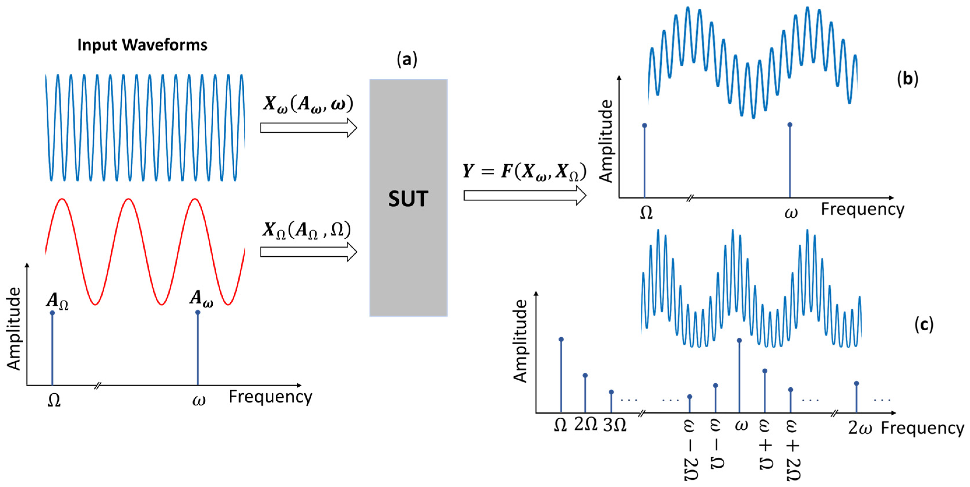
Vibro-Acoustic Modulation (VAM) method, first introduced by Donskoy and Sutin in 1998 [1,2]. In this method, two signals at low (Ω) and high (ω) frequencies, which are called $X_{\mathrm{\Omega }}$ and $X_{\omega }$ as represented in Equation (1), are simultaneously excited to a structure under test (SUT), and another sensor (or sensors) measures a response signal, simultaneously. Furthermore, VAM also shows potential for crack localization [3,4,5,6,7], as first proposed theoretically by Donskoy [2] but not further explored experimentally.

The behavior of the SUT can be described in two different situations: (1) When the structure is perfectly elastic and defect-free, its stress–strain relationship is well-approximated by a linear Hookean law $\sigma \left(\epsilon \right)= E \epsilon$, where $\sigma$, $\epsilon ,$ and $E$ represent stress, strain, and Young’s Modulus, respectively. Under this condition $X_{\Omega }$ and $X_{\omega }$ do not significantly interact, and no sidebands are generated [1,2]. The frequency response of the measured signal reveals only frequency components at $\mathsf{\omega }$ and $\mathsf{\Omega }$, as shown in Figure 1b.

(2) When the structure has a defect such as a crack, the defect introduces a localized nonlinear stress–strain behavior. A simple nonlinear stress–strain can be written using a polynomial expansion, $\sigma \left(\epsilon \right)= E \epsilon + \alpha {\epsilon }^2+ \beta {\epsilon }^3+ \cdots$, where $\alpha$ and $\beta$ are higher-order nonlinear coefficients related to microstructural or contact-type nonlinearity. Under this condition, the high-order polynomial terms in the nonlinear stress–strain expansion generate higher harmonics of $X_{\Omega }$ and $X_{\omega }$ and the sidebands at $\mathsf{\omega }\pm n\mathsf{\Omega }$ [1,2,8,9,10,11,12]. The frequency response of the measured signal in this condition reveals frequency components not only at $\mathsf{\omega }$ and $\mathsf{\Omega }$, but higher harmonics of $\mathsf{\omega }$ and $\mathsf{\Omega }$ as well as $\mathsf{\omega }\pm n\mathsf{\Omega }$, as shown in Figure 1c.

$$\begin{array}{lll}\mathrm{LF} \mathrm{signal}:\hspace{1em}& X_{\mathrm{\Omega }}\left(t\right)\equiv X_{\mathrm{\Omega }}\left(A_{\mathrm{\Omega }},\mathrm{\Omega }\right)=A_{\mathrm{\Omega }}Cos\left(\mathrm{\Omega }t+{\theta }_{\mathrm{\Omega }}\right) , \mathrm{\Omega }=2\mathsf{\pi }{f}_{\mathrm{\Omega }}& \hspace{1em}\mathrm{a}\\ \mathrm{HF} \mathrm{signal}:\hspace{1em}& X_{\omega }\left(t\right)\equiv X_{\omega }\left(A_{\omega },\omega \right)=A_{\omega }Cos\left(\omega t+{\theta }_{\omega }\right), \omega =2\mathsf{\pi }{f}_{\omega }& \hspace{1em}\mathrm{b}\end{array}$$

(1)

Donskoy et al. [13] discussed the nonlinear interaction between ultrasonic waves and low-frequency vibrations at contact interfaces containing defects, such as cracks and delamination, using the VAM technique. By modulating an HF ultrasonic wave with LF vibrations, defect-induced signals can be distinguished from linear acoustic reflections, allowing more sensitive detection. Their results demonstrate how observing sideband components enhances defect identification and may provide insights into defect size and bonding strength.

Duffour et al. [14] examine the effectiveness of VAM for crack detection in metals, focusing on the amplitude modulation of ultrasonic waves (HF signal) by LF vibrations. The authors investigated the relationship between crack size and modulation strength, noting that the correlation is poor due to the sensitivity of the technique to initial crack states and setup conditions.

In another work, Donskoy [15] emphasized that linear methods often miss tiny damages in structures. Nonlinear methods, including harmonic distortion and modulation techniques, exploit stress–strain nonlinearities that become more pronounced in the vicinity of defects such as cracks or delamination.

Aymerich and Staszewski [16] explored cross-modulation vibro-acoustic techniques for detecting impact damage in composite laminates. A slow, amplitude-modulated pumping wave is paired with a constant-amplitude probing wave, producing modulation effects that indicate the presence of damage. The study demonstrated how sidebands in the power spectrum of the probing wave correlate with the severity of barely visible impact damage. Despite boundary condition challenges, the authors validate the flexibility and effectiveness of the technique for early-stage damage detection.

In 2010, Hu et al. [17] investigated nonlinear VAM for crack detection using piezoceramic transducers, focusing on separating amplitude and frequency modulations via the Hilbert–Huang transform (HHT). Their findings show that amplitude modulation correlates more reliably with crack severity than frequency modulation. The authors provided a clear indication of damage progression by isolating the amplitude component.

Donskoy and Ramezani [18] suggested an algorithm to separate amplitude and frequency modulation indices in VAM in 2018. Furthermore, they introduced a Non-Modulated Carrier (NMC), an HF wave part that did not pass through defects and remained non-modulated. The amplitude and phase shift of the NMC change due to wave propagation. Since the modulated signal and NMC have the same primary (carrier) frequency, which is $\omega$, the summation of these signals contaminates the amplitude and the phase shift of the measured signal at the frequency $\omega$. Therefore, they suggested a time-domain algorithm, the Sweeping-Phase Homodyne Separation (SPHS), to separate the amplitude and frequency modulation indices using the first sidebands (left and right) to avoid using the contaminated carrier frequency. The results published by Donskoy and Ramezani showed that the SPHS algorithm can successfully separate the amplitude and frequency modulation indices in the presence of an NMC. Their experimental results revealed that the frequency modulation index (FMI) was larger than the amplitude modulation index (AMI) at the earlier stage of the defect. Then, AMI became larger than FMI at the end of a fatigue damage evolution [18]. In another work in 2019 [19], they reported that early micro-crack stages exhibit mostly frequency modulation, while amplitude modulation becomes pronounced during macro-crack formation.

Klepka et al. [20] examined nonlinear modulation effects in vibro-acoustic tests for detecting contact-type damage using HT. They identified that modulation patterns, notably amplitude and frequency modulations, depend heavily on excitation amplitudes and interactions between low- and high-frequency signals with damaged surfaces.

In 2020, Opperman et al. [21] employed mathematical approaches to explain amplitude and phase modulation, using a short-time Fourier transform (STFT) to estimate them separately. They noted that their results could not confirm whether either AM or PM/FM is a reliable index for revealing a defect.

Gorski et al. [22] investigate the Modulation Transfer (MT) phenomenon, also known as the Luxembourg–Gorky effect, within the context of nonlinear elastic wave theory for damage localization. The authors propose a novel signal processing approach capable of separating Amplitude Modulation (AM) and Frequency Modulation (FM) components from the structural response, based on the HT. They concluded that the observed FM components likely arise from Time-of-Flight (ToF) modulation. They hypothesized that the pumping wave induces stress-dependent variations in wave propagation velocity and path length at the crack interface, which manifests as phase and, consequently, frequency modulation in the probing signal.

In summary, from the literature reviewed, the following challenges or questions regarding defect detection and modulation indices still exist:

• Previous studies in this field have clearly confirmed the presence of at least two types of modulation in the response signal, amplitude modulation and either frequency or phase modulation [11,12,17,18,20,21,22]. However, the possibility of all three modulation types (amplitude, frequency, and phase) coexisting needs further investigation.
• The MI separation techniques proposed by researchers examine the relationship between the nonlinear behavior of the structure under test (SUT) and the corresponding measured response parameters. However, the possibility of early crack detection using these parameters remains to be investigated.
• The proposed methods for MI separation are developed based on the mathematical representation of the modulation phenomena observed in the measured response. The selected model must accurately characterize the response behavior (amplitude and phase shift) throughout its lifetime.
• Although Hilbert transform-based methods have high potential for simultaneously analyzing the amplitude and phase of the measured response, the presence of a non-modulated carrier (NMC) can lead to inaccurate results. Therefore, techniques that provide more reliable results are required.

Despite advancements in modulation indices (MIs) separation and damage-detection techniques, the relationship between MIs and damage progression remains unclear and requires further mathematical clarification. Notably, this relationship highly depends on the chosen signal model and its parameters. In this study, we propose a comprehensive model that integrates amplitude, frequency, and phase modulation simultaneously. This model represents changes in the phase shifts of different frequency components as a function of MIs, as confirmed by experimental results.

2. Methodology

As mentioned earlier, the experimental results [11,12,17,18,20,21,22] confirm the presence of two distinct modulation types, amplitude and frequency/phase modulation, in the VAM-measured response. The easiest way to mathematically describe modulation is to consider a single-tone HF (carrier) signal modulated by a single-tone LF signal. The modulation model must be able to describe changes in the parameters of the measured response (amplitude and phase shift) as MIs vary.

The most commonly employed model for describing the measured signal and MI separation is a combination of amplitude and frequency modulation [17,18]. This model is referred to as AFM in subsequent references. However, this model cannot fully describe the behavior of the measured response over its lifetime, whereas MIs vary. In this research, a combination of all three modulation types (an amplitude–frequency–phase modulation) is introduced and described mathematically. This model is also referred to as AFPM in subsequent references. The following subsections represent both AFM and AFPM models and their differences.

2.1. An Amplitude–Frequency Modulation Model

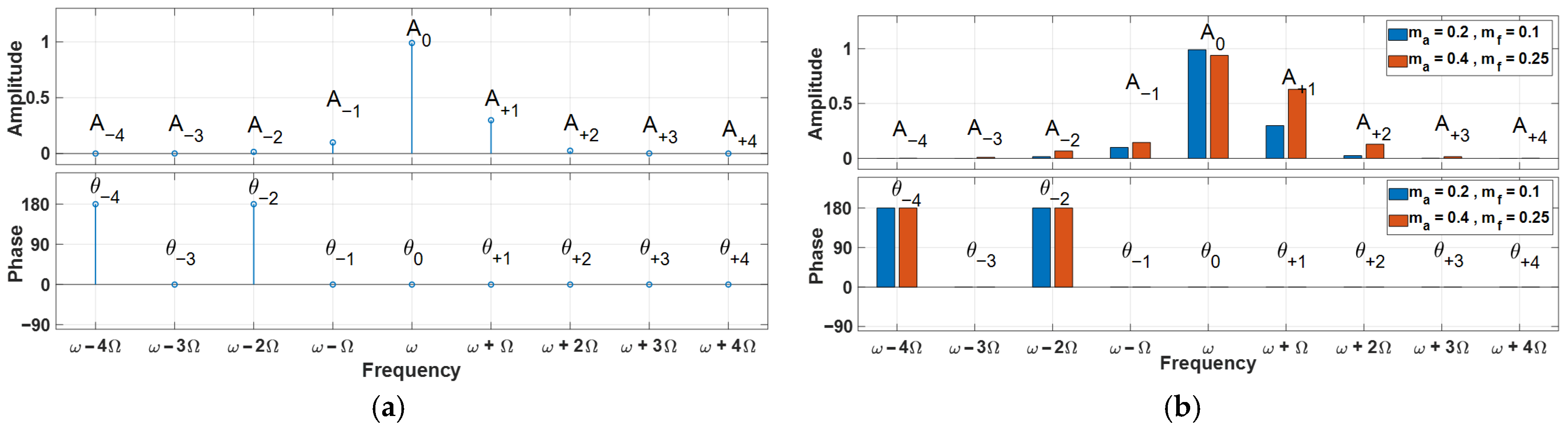
In this modulation, both the amplitude and frequency of the HF signal change based on the LF signal, which is illustrated in Equation (2), where $m_a$ and $m_f$ quantify the amount of amplitude and frequency modulations, respectively. The number of sidebands in this model is theoretically infinite [1,10,13,23,24,25,26], which is shown in Figure 2a.

Table 1. The amplitude and phase shift for different signal components in an amplitude–frequency modulated (AFM) signal when HF and LF signals are single-tone waveforms.

Frequency	Amplitude	Phase Shift
$\omega$	$A_0=A_{\omega }{J}_0\left(2m_f{A}_{\mathrm{\Omega }}\right)$	${\theta }_0={\varphi }_{\omega }$
$\omega +\mathsf{\Omega }$	$A_{+1}=A_{\omega }\left(J_1\left(2m_f{A}_{\mathrm{\Omega }}\right)+m_a{A}_{\mathrm{\Omega }}{J}_0\left(2m_f{A}_{\mathrm{\Omega }}\right)+m_a{A}_{\mathrm{\Omega }}{J}_2\left(2m_f{A}_{\mathrm{\Omega }}\right)\right)$	${\theta }_{+1}={\varphi }_{\omega }+{\varphi }_{\mathsf{\Omega }}$
$\omega -\mathsf{\Omega }$	$A_{-1}=A_{\omega }\left(-J_1\left(2m_f{A}_{\mathrm{\Omega }}\right)+m_a{A}_{\mathrm{\Omega }}{J}_0\left(2m_f{A}_{\mathrm{\Omega }}\right)+m_a{A}_{\mathrm{\Omega }}{J}_2\left(2m_f{A}_{\mathrm{\Omega }}\right)\right)$	${\theta }_{-1}={\varphi }_{\omega }-{\varphi }_{\mathsf{\Omega }}$
$\omega +2\mathsf{\Omega }$	$A_{+2}=A_{\omega }\left(J_2\left(2m_f{A}_{\mathrm{\Omega }}\right)+m_a{A}_{\mathrm{\Omega }}{J}_1\left(2m_f{A}_{\mathrm{\Omega }}\right)+m_a{A}_{\mathrm{\Omega }}{J}_3\left(2m_f{A}_{\mathrm{\Omega }}\right)\right)$	${\theta }_{+2}={\varphi }_{\omega }+2{\varphi }_{\mathsf{\Omega }}$
$\omega -2\mathsf{\Omega }$	$A_{-2}=A_{\omega }\left(J_2\left(2m_f{A}_{\mathrm{\Omega }}\right)-m_a{A}_{\mathrm{\Omega }}{J}_1\left(2m_f{A}_{\mathrm{\Omega }}\right)-m_a{A}_{\mathrm{\Omega }}{J}_3\left(2m_f{A}_{\mathrm{\Omega }}\right)\right)$	${\theta }_{-2}={\varphi }_{\omega }-2{\varphi }_{\mathsf{\Omega }}$
$\omega +n\mathsf{\Omega }$	$A_{+n}=A_{\omega }\left(J_n\left(2m_f{A}_{\mathrm{\Omega }}\right)+m_a{A}_{\mathrm{\Omega }}{J}_{n-1}\left(2m_f{A}_{\mathrm{\Omega }}\right)+m_a{A}_{\mathrm{\Omega }}{J}_{n+1}\left(2m_f{A}_{\mathrm{\Omega }}\right)\right)$	${\theta }_{+n}={\varphi }_{\omega }+n{\varphi }_{\mathsf{\Omega }}$
$\omega -n\mathsf{\Omega }$	$A_{+n}={\left(-1\right)}^n{A}_{\omega }\left(J_n\left(2m_f{A}_{\mathrm{\Omega }}\right)-m_a{A}_{\mathrm{\Omega }}{J}_{n-1}\left(2m_f{A}_{\mathrm{\Omega }}\right)-m_a{A}_{\mathrm{\Omega }}{J}_{n+1}\left(2m_f{A}_{\mathrm{\Omega }}\right)\right)$	${\theta }_{-n}={\varphi }_{\omega }-n{\varphi }_{\mathsf{\Omega }}$

represents the amplitude and phase shift of the AFM signal components after replacing $X_{\mathsf{\Omega }}\left(t\right)$, defined in Equation (1), into the Equation (2). As evident in Table 1, the phase shifts of the signal components remain unchanged despite changes in the MIs, and the amplitude of the corresponding sidebands ($\left|A_{\pm \mathrm{n}}\right|$) are not symmetric in this model (see Figure 2b). It is noticeable that the amplitude of the corresponding sidebands ($\left|A_{\pm \mathrm{n}}\right|$) are symmetric in an amplitude and phase modulation model.

$$A_{\omega }\left(1+2m_a{X}_{\mathsf{\Omega }}\left(t\right)\right)\mathit{cos}\left(\omega t+{\varphi }_{\omega }+2m_f \int X_{\mathsf{\Omega }}\left(t\right)dt\right)$$

(2)

2.2. An Amplitude–Frequency–Phase Modulation Model

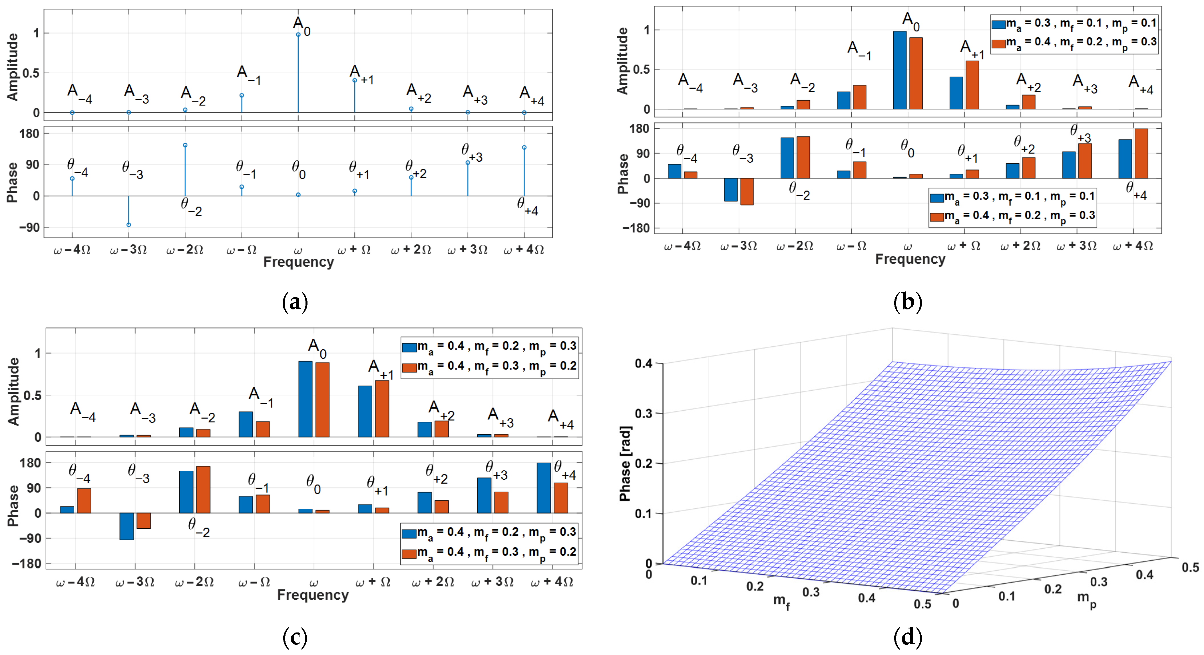
The mathematical description of this model is not presented in reference books and is presented here for the first time. In this model, the amplitude, frequency, and phase of the HF signal change based on the LF signal, which is illustrated in Equation (3), where $m_a,m_f$, and $m_p$, quantifies amplitude, frequency, and phase modulations. This model can be converted to an Amplitude–Phase modulated signal with a new modulation index by using some trigonometric identities illustrated in Equation (4). The number of sidebands in this model is also theoretically infinite, as shown in Figure 3a.

Table 2. The amplitude of different signal components in an AFPM signal when HF and LF signals are single-tone waveforms, where $z=2A_{\mathsf{\Omega }}\sqrt{{m_f}^2+{m_p}^2}$ and $\beta ={\mathit{tan}}^{-1}\left({\displaystyle \frac{m_f}{m_p}}\right)$.

Frequency	Amplitude
$\omega$	$A_0=A_{\omega }\sqrt{{\left(a_0\right)}^2+{\left(b_0\right)}^2}$	$a_0=J_0\left(z\right)$
		$b_0=-2m_a{A}_{\mathsf{\Omega }}{J}_1\left(z\right)\mathit{cos}\left(\beta \right)$
$\omega +\mathsf{\Omega }$	$A_{+1}=A_{\omega }\sqrt{{\left(a_{+1}\right)}^2+{\left(b_{+1}\right)}^2}$	$a_{+1}=m_a{A}_{\mathsf{\Omega }}{J}_0\left(z\right)-m_a{A}_{\mathsf{\Omega }}{J}_2\left(z\right)\mathit{cos}\left(2\beta \right)+J_1\left(z\right)\mathit{sin}\left(\beta \right)$
		$b_{+1}=-m_a{A}_{\mathsf{\Omega }}{J}_2\left(z\right)\mathit{sin}\left(2\beta \right)-J_1\left(z\right)\mathit{cos}\left(\beta \right)$
$\omega -\mathsf{\Omega }$	$A_{-1}=A_{\omega }\sqrt{{\left(a_{+1}\right)}^2+{\left(b_{+1}\right)}^2}$	$a_{-1}=m_a{A}_{\mathsf{\Omega }}{J}_0\left(z\right)-m_a{A}_{\mathsf{\Omega }}{J}_2\left(z\right)\mathit{cos}\left(2\beta \right)-J_1\left(z\right)\mathit{sin}\left(\beta \right)$
		$b_{-1}=m_a{A}_{\mathsf{\Omega }}{J}_2\left(z\right)\mathit{sin}\left(2\beta \right)-J_1\left(z\right)\mathit{cos}\left(\beta \right)$
$\omega +2\mathsf{\Omega }$	$A_{+2}=A_{\omega }\sqrt{{\left(a_{+1}\right)}^2+{\left(b_{+1}\right)}^2}$	$a_{+2}=-J_2\left(z\right)\mathit{cos}\left(2\beta \right)+m_a{A}_{\mathsf{\Omega }}{J}_1\left(z\right)\mathit{sin}\left(\beta \right)-m_a{A}_{\mathsf{\Omega }}{J}_3\left(z\right)\mathit{sin}\left(3\beta \right)$
		$b_{+2}=-J_2\left(z\right)\mathit{sin}\left(2\beta \right)-m_a{A}_{\mathsf{\Omega }}{J}_1\left(z\right)\mathit{cos}\left(\beta \right)+m_a{A}_{\mathsf{\Omega }}{J}_3\left(z\right)\mathit{cos}\left(3\beta \right)$
$\omega -2\mathsf{\Omega }$	$A_{-2}=A_{\omega }\sqrt{{\left(a_{+1}\right)}^2+{\left(b_{+1}\right)}^2}$	$a_{-2}=-J_2\left(z\right)\mathit{cos}\left(2\beta \right)-m_a{A}_{\mathsf{\Omega }}{J}_1\left(z\right)\mathit{sin}\left(\beta \right)+m_a{A}_{\mathsf{\Omega }}{J}_3\left(z\right)\mathit{sin}\left(3\beta \right)$
		$b_{-2}=J_2\left(z\right)\mathit{sin}\left(2\beta \right)-m_a{A}_{\mathsf{\Omega }}{J}_1\left(z\right)\mathit{cos}\left(\beta \right)+m_a{A}_{\mathsf{\Omega }}{J}_3\left(z\right)\mathit{cos}\left(3\beta \right)$

and

Table 3. The phase shift of different signal components in an AFPM signal.

Frequency	Phase Shift
$\omega$	${\theta }_0={\varphi }_{\omega }-{\mathit{tan}}^{-1}\left({\displaystyle \frac{b_0}{a_0}}\right)$	$a_0=J_0\left(z\right)$
		$b_0=-2m_a{A}_{\mathsf{\Omega }}{J}_1\left(z\right)\mathit{cos}\left(\beta \right)$
$\omega +\mathsf{\Omega }$	${\theta }_{+1}={\varphi }_{\omega }+{\varphi }_{\mathsf{\Omega }}-{\mathit{tan}}^{-1}\left({\displaystyle \frac{b_{+1}}{a_{+1}}}\right)$	$a_{+1}=m_a{A}_{\mathsf{\Omega }}{J}_0\left(z\right)-m_a{A}_{\mathsf{\Omega }}{J}_2\left(z\right)\mathit{cos}\left(2\beta \right)+J_1\left(z\right)\mathit{sin}\left(\beta \right)$
		$b_{+1}=-m_a{A}_{\mathsf{\Omega }}{J}_2\left(z\right)\mathit{sin}\left(2\beta \right)-J_1\left(z\right)\mathit{cos}\left(\beta \right)$
$\omega -\mathsf{\Omega }$	${\theta }_{-1}={\varphi }_{\omega }-{\varphi }_{\mathsf{\Omega }}-{\mathit{tan}}^{-1}\left({\displaystyle \frac{b_{-1}}{a_{-1}}}\right)$	$a_{-1}=m_a{A}_{\mathsf{\Omega }}{J}_0\left(z\right)-m_a{A}_{\mathsf{\Omega }}{J}_2\left(z\right)\mathit{cos}\left(2\beta \right)-J_1\left(z\right)\mathit{sin}\left(\beta \right)$
		$b_{-1}=m_a{A}_{\mathsf{\Omega }}{J}_2\left(z\right)\mathit{sin}\left(2\beta \right)-J_1\left(z\right)\mathit{cos}\left(\beta \right)$
$\omega +2\mathsf{\Omega }$	${\theta }_{+2}={\varphi }_{\omega }+2{\varphi }_{\mathsf{\Omega }}-{\mathit{tan}}^{-1}\left({\displaystyle \frac{b_{+2}}{a_{+2}}}\right)$	$a_{+2}=-J_2\left(z\right)\mathit{cos}\left(2\beta \right)+m_a{A}_{\mathsf{\Omega }}{J}_1\left(z\right)\mathit{sin}\left(\beta \right)-m_a{A}_{\mathsf{\Omega }}{J}_3\left(z\right)\mathit{sin}\left(3\beta \right)$
		$b_{+2}=-J_2\left(z\right)\mathit{sin}\left(2\beta \right)-m_a{A}_{\mathsf{\Omega }}{J}_1\left(z\right)\mathit{cos}\left(\beta \right)+m_a{A}_{\mathsf{\Omega }}{J}_3\left(z\right)\mathit{cos}\left(3\beta \right)$
$\omega -2\mathsf{\Omega }$	${\theta }_{-2}={\varphi }_{\omega }-2{\varphi }_{\mathsf{\Omega }}-{\mathit{tan}}^{-1}\left({\displaystyle \frac{b_{-2}}{a_{-2}}}\right)$	$a_{-2}=-J_2\left(z\right)\mathit{cos}\left(2\beta \right)-m_a{A}_{\mathsf{\Omega }}{J}_1\left(z\right)\mathit{sin}\left(\beta \right)+m_a{A}_{\mathsf{\Omega }}{J}_3\left(z\right)\mathit{sin}\left(3\beta \right)$
		$b_{-2}=J_2\left(z\right)\mathit{sin}\left(2\beta \right)-m_a{A}_{\mathsf{\Omega }}{J}_1\left(z\right)\mathit{cos}\left(\beta \right)+m_a{A}_{\mathsf{\Omega }}{J}_3\left(z\right)\mathit{cos}\left(3\beta \right)$

represent the amplitude and phase shift of the AFPM signal components after replacing $X_{\mathsf{\Omega }}\left(t\right)$, defined in Equation (1), into Equation (3). As evident in Table 2 and Table 3, the phase shifts and the amplitude of the signal components vary with the change in the modulation indices (see Figure 3b,d), and the amplitude of the corresponding sidebands ($\left|A_{\pm \mathrm{n}}\right|$) are not symmetric in this model.

$$A_{\omega }\left(1+2m_a{X}_{\mathsf{\Omega }}\left(t\right)\right)\mathit{cos}\left(2\pi f_{\omega }t+{\varphi }_{\omega }+2m_p X_{\mathsf{\Omega }}\left(t\right)+2m_f \int X_{\mathsf{\Omega }}\left(t\right)dt\right)$$

(3)

$$A_{\omega }\left(1+2m_a{A}_{\mathsf{\Omega }}\mathit{cos}\left(\mathsf{\Omega }t+{\varphi }_{\mathsf{\Omega }}\right)\right)\mathit{cos}\left(\omega t+{\varphi }_{\omega }+2m_p A_{\mathsf{\Omega }}\mathit{cos}\left(\mathsf{\Omega }t+{\varphi }_{\mathsf{\Omega }}\right)+2m_f A_{\mathsf{\Omega }}\mathit{sin}\left(\mathsf{\Omega }t+{\varphi }_{\mathsf{\Omega }}\right)\right)$$

$$A_{\omega }\left(1+2m_a{A}_{\mathsf{\Omega }}\mathit{cos}\left(\mathsf{\Omega }t+{\varphi }_{\mathsf{\Omega }}\right)\right)\mathit{cos}\left(\omega t+{\varphi }_{\omega }+2A_{\mathsf{\Omega }}\sqrt{{m_f}^2+{m_p}^2} \mathit{cos}\left(\mathsf{\Omega }t+{\varphi }_{\mathsf{\Omega }}-{\mathit{tan}}^{-1}\left({\displaystyle \frac{m_f}{m_p}}\right) \right) \right)$$

(4)

2.3. The Phase Shifts Are the Distinguishing Feature

The amplitude of the frequency spectrum of the measured response is insufficient for determining the appropriate modulation model. As shown in Figure 2a and Figure 3a, both AFM and AFPM have the same features: (1) infinite sidebands and (2) non-symmetrical sideband amplitudes. Therefore, the phase of the frequency spectrum of the measured response must also be considered in this decision.

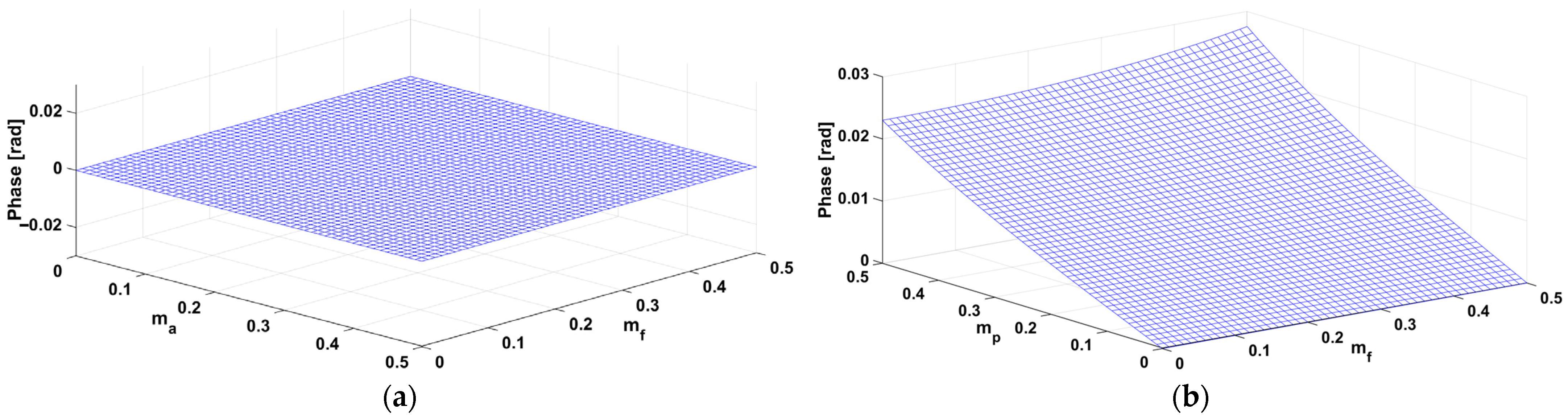
As shown in Table 3, all signal components in the AFPM model exhibit an additional phase shift related to the MIs. However, the phase shift of all components for the AFM model remains constant with changes in $m_a$ or $m_f$. Figure 4 shows an example of 3D plots of the phase shift of a MATLAB-simulated signal at the primary frequency, ${\varphi }_{\omega }$, for both AFM and AFPM models (see Table 1 and Table 3).

Experimental results [10,17,18,19,20] confirmed that MIs evolve over the lifetime of the SUT. Consequently, variations in the phase shift of different frequency components within the measured response provide clear evidence supporting the possible coexistence of all three modulation types.

2.4. Relative Sensitivity of the DMI and Phase Shifts

Researchers have suggested different parameters to quantify the effect of a defect on the system response. The most popular parameter quantifying modulation is the Damage Modulation Index (DMI), defined by Donskoy [1] and given in Equation (5), where $A_{\pm \mathrm{1,0}}$ represent the amplitude of sidebands and the primary frequency defined before [1,10,27,28]. This parameter was initially called Modulation Index (MI) by Donskoy, but will be called the Damage Modulation Index (DMI), to avoid overlapping with the signal modulation index.

$$DMI={\displaystyle \frac{A_{+1}+A_{-1}}{2A_0}}$$

(5)

The sensitivity of phase shifts and DMI to changes in modulation index can be investigated by examining the relative sensitivities of both functions. The relative sensitivity (RS) of a function to its variable is given in Equation (6).

$$Relative Sensitivity of F\left(x_1,x_2,x_3,\dots ,x_n\right) to x_k \equiv S_{x_k}^F={\displaystyle \frac{\mathsf{\partial }F}{\mathsf{\partial }{x}_k}} {\displaystyle \frac{x_k}{F}}$$

(6)

Equations (7) and (8) represent the relationship between DMI and the summation of phase shifts of the first sidebands See Section 3.3, $\mathsf{\Phi }$, as functions of MIs for an AFPM model, where $A_{+1}$, $A_{-1}$, $A_0$, ${\theta }_{+1}$, ${\theta }_{-1}$, $\beta$ and $z$ are represented in Table 2 and Table 3.

$$DMI\left(m_a,m_f,m_p\right)={\displaystyle \frac{A_{+1}+A_{-1}}{2A_0}}$$

$$DMI= {\displaystyle \frac{\sqrt{{\left(m_a{A}_{\mathsf{\Omega }}\right)}^2{\left(J_0-J_2\right)}^2{\cos }^2\beta +{\left(m_a{A}_{\mathsf{\Omega }}\left(J_0+J_2\right)\sin \beta +J_1\right)}^2}+\sqrt{{\left(m_a{A}_{\mathsf{\Omega }}\right)}^2{\left(J_0-J_2\right)}^2{\cos }^2\beta +{\left(m_a{A}_{\mathsf{\Omega }}\left(J_0+J_2\right)\sin \beta -J_1\right)}^2}}{2\hspace{0.17em}\sqrt{J_0^2+4\hspace{0.17em}{\left(m_a{A}_{\mathsf{\Omega }}\right)}^2\hspace{0.17em}{J}_1^2{\cos }^2\beta }}}$$

(7)

$$\mathsf{\Phi }\left(m_a,m_f,m_p\right)={\theta }_{+1}+{\theta }_{-1}$$

$$\mathsf{\Phi }=-{\mathit{tan}}^{-1}\left({\displaystyle \frac{b_{+1}}{a_{+1}}}\right)-{\mathit{tan}}^{-1}\left({\displaystyle \frac{b_{-1}}{a_{-1}}}\right)$$

$$\mathsf{\Phi }=-{\mathit{tan}}^{-1}\left({\displaystyle \frac{-m_a{A}_{\mathsf{\Omega }}{J}_2\left(z\right)\mathit{sin}\left(2\beta \right)-J_1\left(z\right)\mathit{cos}\left(\beta \right)}{m_a{A}_{\mathsf{\Omega }}{J}_0\left(z\right)-m_a{A}_{\mathsf{\Omega }}{J}_2\left(z\right)\mathit{cos}\left(2\beta \right)+J_1\left(z\right)\mathit{sin}\left(\beta \right)}}\right)-{\mathit{tan}}^{-1}\left({\displaystyle \frac{m_a{A}_{\mathsf{\Omega }}{J}_2\left(z\right)\mathit{sin}\left(2\beta \right)-J_1\left(z\right)\mathit{cos}\left(\beta \right)}{m_a{A}_{\mathsf{\Omega }}{J}_0\left(z\right)-m_a{A}_{\mathsf{\Omega }}{J}_2\left(z\right)\mathit{cos}\left(2\beta \right)-J_1\left(z\right)\mathit{sin}\left(\beta \right)}}\right)$$

(8)

The RS of both DMI and $\mathsf{\Phi }$ for each MI can be calculated using Equation (6). Finally, the second norm (${‖f‖}_2=\sqrt{\sum {\left|f_i\right|}^2}, where f=\left[f_1,f_2,f_3,\dots ,f_n\right]$) for each MI is calculated as the RS of DMI and $\mathsf{\Phi }$, as given in Equations (9) and (10).

$$Relative Sensitivity of DMI=\sqrt{{\left({\displaystyle \frac{\mathsf{\partial }DMI}{\mathsf{\partial }{m}_a}} {\displaystyle \frac{m_a}{DMI}}\right)}^2+{\left({\displaystyle \frac{\mathsf{\partial }DMI}{\mathsf{\partial }{m}_f}} {\displaystyle \frac{m_f}{DMI}}\right)}^2+{\left({\displaystyle \frac{\mathsf{\partial }DMI}{\mathsf{\partial }{m}_p}} {\displaystyle \frac{m_p}{DMI}}\right)}^2}$$

(9)

$$Relative Sensitivity of \mathsf{\Phi }=\sqrt{{\left({\displaystyle \frac{\mathsf{\partial }\mathsf{\Phi }}{\mathsf{\partial }{m}_a}} {\displaystyle \frac{m_a}{\mathsf{\Phi }}}\right)}^2+{\left({\displaystyle \frac{\mathsf{\partial }\mathsf{\Phi }}{\mathsf{\partial }{m}_f}} {\displaystyle \frac{m_f}{\mathsf{\Phi }}}\right)}^2+{\left({\displaystyle \frac{\mathsf{\partial }\mathsf{\Phi }}{\mathsf{\partial }{m}_p}} {\displaystyle \frac{m_p}{\mathsf{\Phi }}}\right)}^2}$$

(10)

MATLAB 2024b was used to numerically evaluate and compare the relative sensitivities of the DMI and $\mathsf{\Phi }$ with respect to variations in the variables. Since RS depends on three variables $m_a$, $m_f$ and $m_p$, a complete visualization would be four-dimensional. To simplify plotting, the parameter $m_a$ is held fixed, and a three-dimensional surface is rendered over $\left(m_f,m_p\right)$. At each simulation step, a value is assigned to $m_a$ and the RS is computed. This procedure is then repeated for multiple $m_a$ values. The ranges and magnitudes of the variable changes are represented in

Table 4. The details of the variables used in the relative sensitivity calculation using MATLAB.

Variable	Min	Step	Max
$m_a$	$1\times {10}^{-6}$	$1\times {10}^{-5}$	$1\times {10}^{-3}$
$m_p$	$1\times {10}^{-6}$	$1\times {10}^{-5}$	$1\times {10}^{-3}$
$m_f$	$1\times {10}^{-6}$	$1\times {10}^{-5}$	$1\times {10}^{-3}$

.

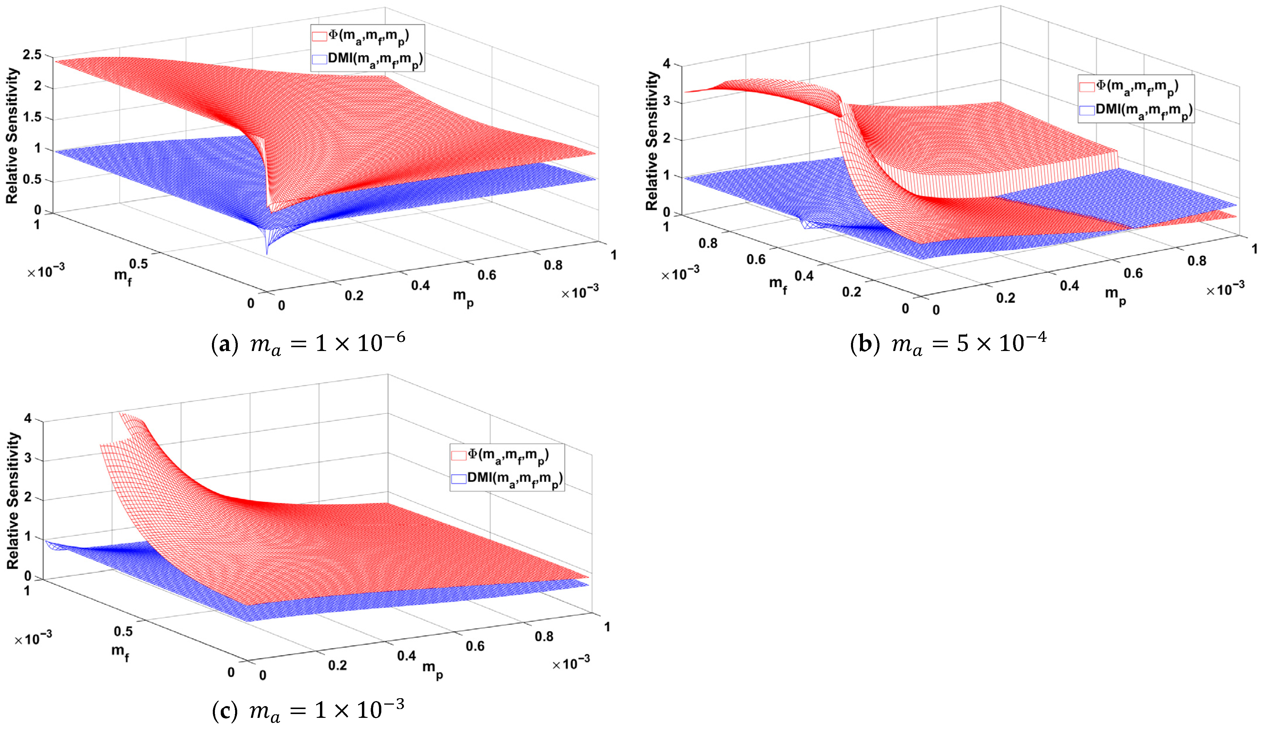
Figure 5 illustrates the 3D plot of the RS for both $DMI\left(m_a,m_f,m_p\right)$ and $\mathsf{\Phi }\left(m_a,m_f,m_p\right)$ in three different values of $m_a$. As it is evident, the RS value of $\mathsf{\Phi }\left(m_a,m_f,m_p\right)$ is bigger than $DMI\left(m_a,m_f,m_p\right)$, which means that the $\mathsf{\Phi }\left(m_a,m_f,m_p\right)$ is more sensitive than $DMI\left(m_a,m_f,m_p\right)$ when any of the MIs change.

The higher sensitivity of $\mathsf{\Phi }\left(m_a,m_f,m_p\right)$ compared with $DMI\left(m_a,m_f,m_p\right)$ implies that variations in the MIs induce larger changes in $\mathsf{\Phi }\left(m_a,m_f,m_p\right)$, which can be exploited for early defect detection. However, it should be emphasized that at the early stage of crack initiation, the variation in phase shift or amplitude of different frequency components is insignificant and may be masked by noise or measurement errors. Utilizing high-precision instrumentation in conjunction with robust noise-reduction techniques can enhance the reliability of the results.

3. Experimental Results

To experimentally validate the applicability of the AFPM model, this section investigates whether the model can capture phase-shift variations in the VAM response induced by changes in MIs. Unlike the AFM model, the AFPM model predicts that the phase shifts of frequency components vary with the MIs.

Table 5. The phase shifts at different frequency components in the AFM and AFPM models.

Frequency	Phase Shifts in the
	AFM Model	AFPM Model
$\omega$	${\varphi }_{\omega }$	${\theta }_0={\varphi }_{\omega }-{\mathit{tan}}^{-1}\left({\displaystyle \frac{-2m_a{A}_{\mathsf{\Omega }}{J}_1\left(z\right)\mathit{cos}\left(\beta \right)}{J_0\left(z\right)}}\right)$
		${\theta }_0={\varphi }_{\omega }+{{\theta }_{MP}}_0$
$\omega +\mathsf{\Omega }$	${\varphi }_{\omega }+{\varphi }_{\mathsf{\Omega }}$	${\theta }_{+1}={\varphi }_{\omega }+{\varphi }_{\mathsf{\Omega }}-{\mathit{tan}}^{-1}\left({\displaystyle \frac{-m_a{A}_{\mathsf{\Omega }}{J}_2\left(z\right)\mathit{sin}\left(2\beta \right)-J_1\left(z\right)\mathit{cos}\left(\beta \right)}{m_a{A}_{\mathsf{\Omega }}{J}_0\left(z\right)-m_a{A}_{\mathsf{\Omega }}{J}_2\left(z\right)\mathit{cos}\left(2\beta \right)+J_1\left(z\right)\mathit{sin}\left(\beta \right)}}\right)$
		${\theta }_{+1}={\varphi }_{\omega }+{\varphi }_{\mathsf{\Omega }}+{{\theta }_{MP}}_{+1}$
$\omega -\mathsf{\Omega }$	${\varphi }_{\omega }-{\varphi }_{\mathsf{\Omega }}$	${\theta }_{-1}={\varphi }_{\omega }-{\varphi }_{\mathsf{\Omega }}-{\mathit{tan}}^{-1}\left({\displaystyle \frac{m_a{A}_{\mathsf{\Omega }}{J}_2\left(z\right)\mathit{sin}\left(2\beta \right)-J_1\left(z\right)\mathit{cos}\left(\beta \right)}{m_a{A}_{\mathsf{\Omega }}{J}_0\left(z\right)-m_a{A}_{\mathsf{\Omega }}{J}_2\left(z\right)\mathit{cos}\left(2\beta \right)-J_1\left(z\right)\mathit{sin}\left(\beta \right)}}\right)$
		${\theta }_{-1}={\varphi }_{\omega }-{\varphi }_{\mathsf{\Omega }}+{{\theta }_{MP}}_{-1}$

provides a direct comparison of the theoretical phase shifts predicted by both models. The following experimental procedure is designed to isolate and evaluate these shifts, thereby confirming the presence of phase-modulation.

3.1. Test Setup

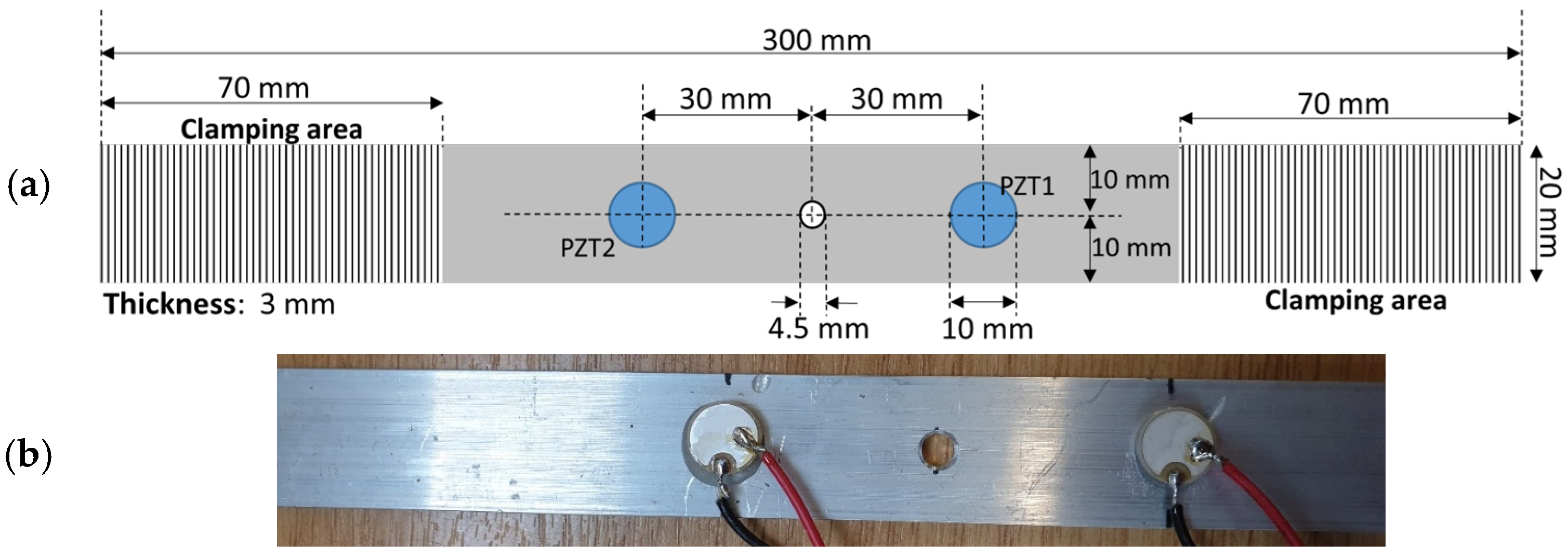
The variation in phase shift of the VAM response is experimentally investigated using aluminum specimens with a thickness of 3 mm, as shown in Figure 6. Two piezoceramics (PI255) with a diameter of 10 mm are attached to one side of the sample to excite the HF signal and measure the system response simultaneously.

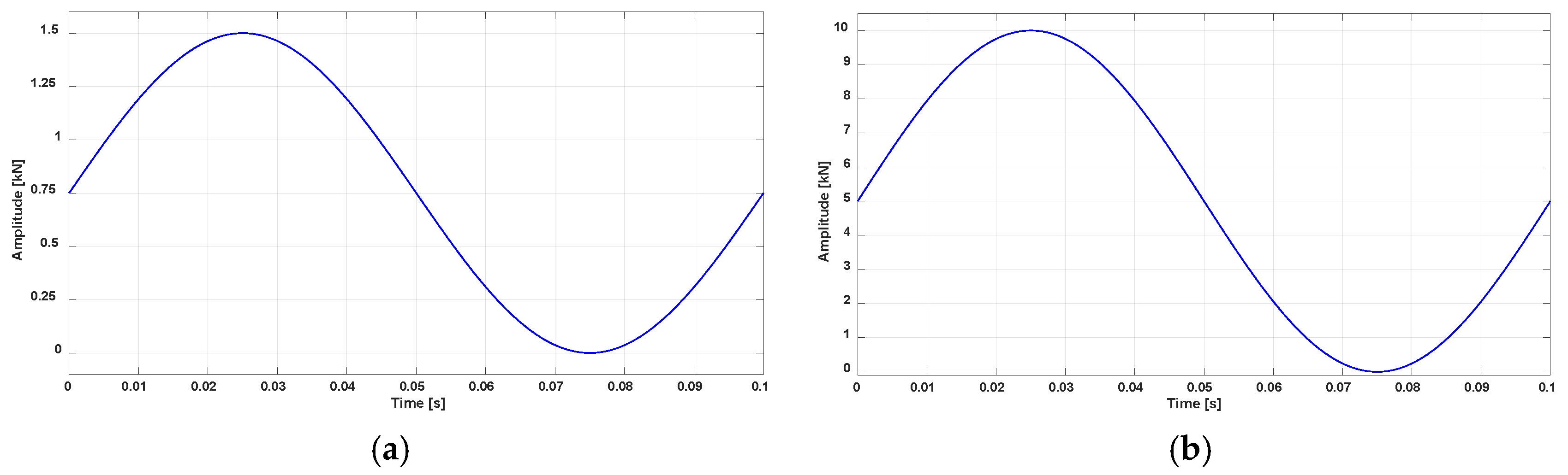
The LF signal is applied using a tensile hydraulic machine, INSTRON 250 kN, at a frequency of $f_{\mathsf{\Omega }}=10 \mathrm{Hz}$ and the amplitude of 1.5 kN (0–1.5 kN), as shown in Figure 7a. After measuring the VAM response for all selected frequencies, the amplitude of the LF is changed to 10 kN (0–10 kN) to induce fatigue in the SUT for a certain number of cycles, as shown in Figure 7b. The procedure repeats until the sample breaks. A National Instruments Multifunction I/O device, USB-6366, is used to send the signal into the actuator and measure the system response simultaneously, and a MATLAB script controls the process.

3.2. High Frequency Selection

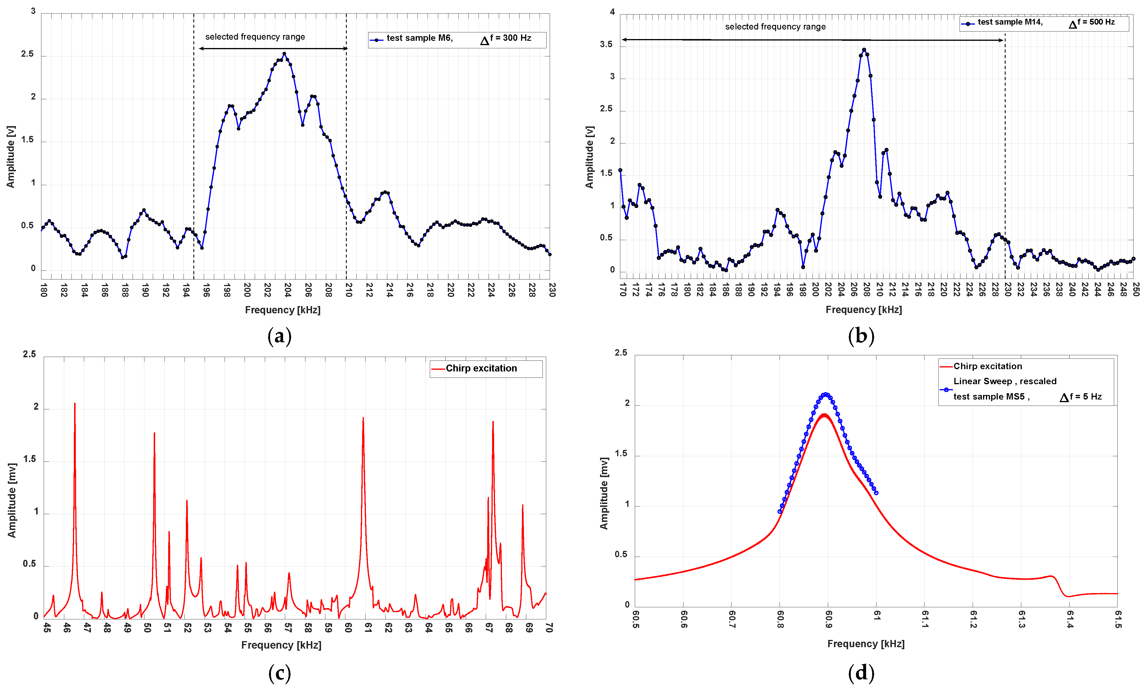
A single-tone HF signal at a specific frequency is generated in MATLAB and applied to the actuator on the sample using an NI device. The signal at the receiver is measured simultaneously. The amplitude of the measured signal, calculated by the FFT, is saved in a matrix. The process of sending and measuring the HF signal is repeated over a specific range of frequencies. A sample of the linear sweep result is shown in Figure 8a,b. A frequency or range of frequencies with high amplitudes is selected at the receiver for the VAM measurement process. The frequency selection can also be achieved using chirp excitation, as illustrated in Figure 8c. As shown in Figure 8d, an eigenfrequency of the sample can also be detected using single-tone excitation (known as a linear sweep method).

3.3. Angle Modulation Phase Shift

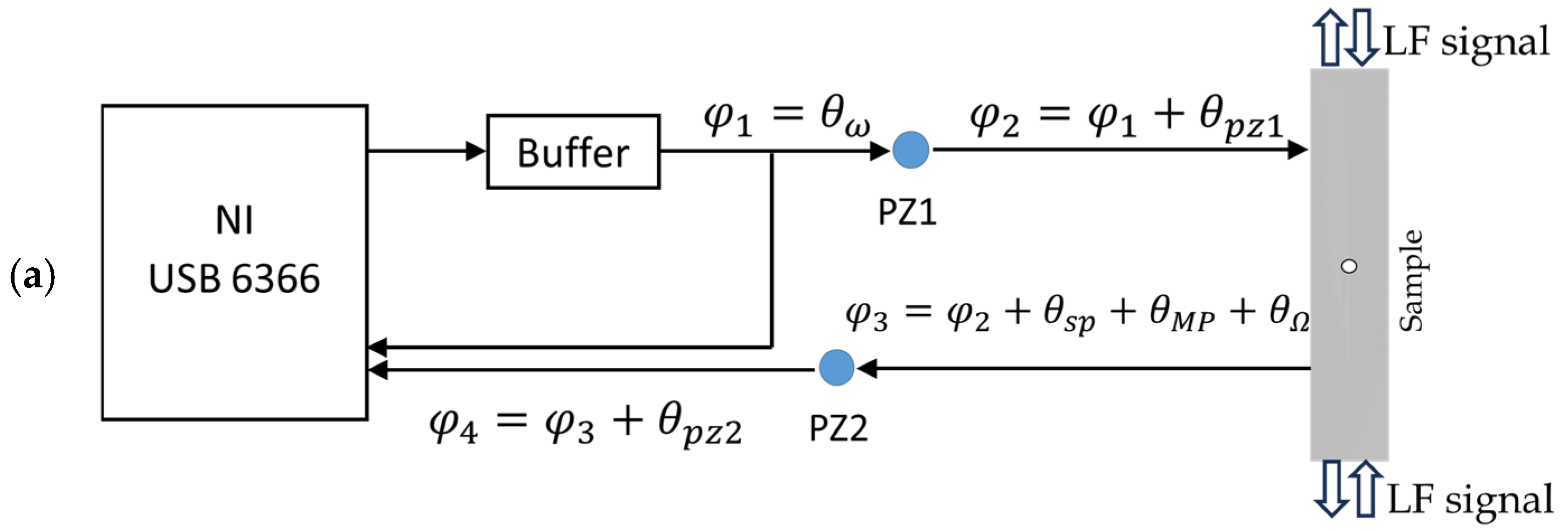
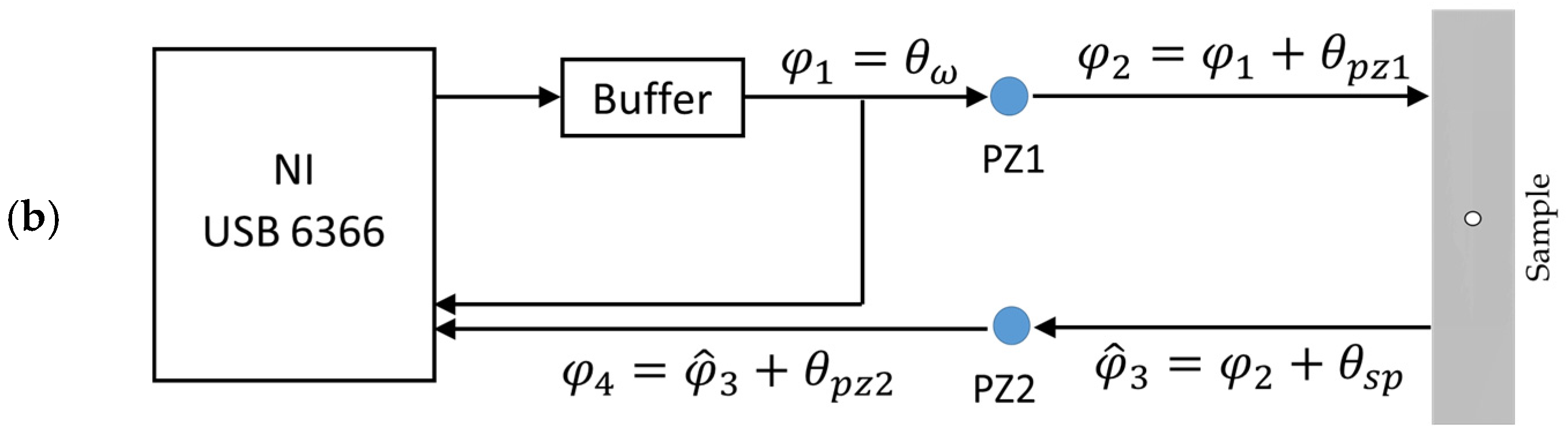
To investigate the phase shift of the VAM response, a test setup, represented in Figure 9, is prepared to measure the VAM response of a sample and the sent HF signal simultaneously. The phase shifts that are written in the figure are introduced in the following:

• ${\theta }_{\omega }$ represents the HF signal phase shift. The value of the ${\theta }_{\omega }$ is arbitrary.
• ${\theta }_{\mathsf{\Omega }}$ represents the LF signal phase shift. The value of the ${\theta }_{\mathsf{\Omega }}$ is arbitrary.
• ${\theta }_{pz1-2}$ represents the change in signal phase shift due to a piezoelectric.
• ${\theta }_{sp}$ represents the signal phase shift introduced by the sample, such as propagation delay.
• ${\theta }_{MP}$ represents the change in signal phase shift due to the modulation itself (see Table 3).

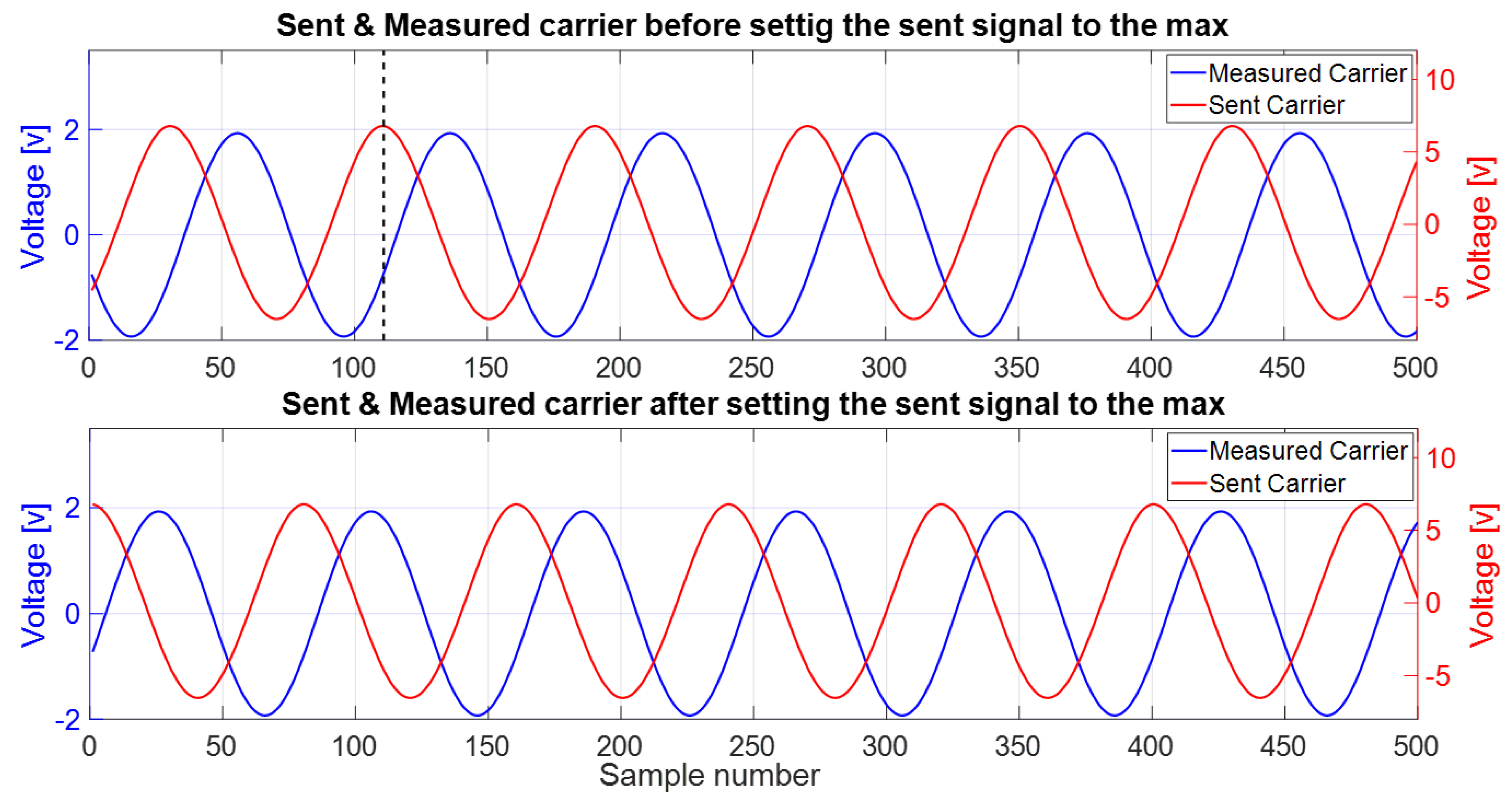
The phase shift of the first sideband was selected for investigation in this test setup to avoid contamination of the measured response by the non-modulated carrier (NMC) component. The value of ${\theta }_{\omega }$, ${\theta }_{pz1-2}$ and ${\theta }_{sp}$ are arbitrary and ${\theta }_{MP}$ is the phase shift that is being calculated. Since the sent signal and response were measured simultaneously, the value of ${\theta }_{\omega }$ can be set to 0 by comparing the sent and measured responses, as represented in Figure 10, or can be eliminated by subtracting the sent signal phase shift calculated by FFT from the measured response phase shift at the end of the phase calculation. Thus, the value of ${\theta }_{\omega }$ is assumed to be 0 for subsequent calculations to simplify.

The phase shift of the VAM response signal at $\omega \pm \mathsf{\Omega }$ using the phase shifts listed in Figure 8a is given in Equation (11). Using the ${\theta }_{+1}+{\theta }_{-1}$ helps us to delete the value ${\theta }_{\mathsf{\Omega }}$ of the equations, especially considering that the value of ${\theta }_{\mathsf{\Omega }}$ is unidentified, as represented in Equation (12).

$$\begin{array}{cc}{\theta }_{+1}={\theta }_{\omega }+{\theta }_{\mathsf{\Omega }}+{\theta }_{pz1}+{\theta }_{pz2}+{{\theta }_{sp}}_{+1}+{{\theta }_{MP}}_{+1}& \hspace{1em}\hspace{1em}\left(\mathrm{a}\right)\\ {\theta }_{-1}={\theta }_{\omega }-{\theta }_{\mathsf{\Omega }}+{\theta }_{pz1}+{\theta }_{pz2}+{{\theta }_{sp}}_{-1}+{{\theta }_{MP}}_{-1}& \hspace{1em}\hspace{1em}\left(\mathrm{b}\right)\end{array}$$

(11)

$${\theta }_{+1}+{\theta }_{-1}=\left({\theta }_{\omega }+{\theta }_{pz1}+{\theta }_{pz2}+{{\theta }_{sp}}_{+1}\right)+\left({\theta }_{\omega }+{\theta }_{pz1}+{\theta }_{pz2}+{{\theta }_{sp}}_{-1}\right)+\left({{\theta }_{MP}}_{+1}+{{\theta }_{MP}}_{-1}\right)$$

(12)

The phase shift of the HF response signal at $\omega$ using the phase shifts listed in Figure 8b is given in Equation (13). By comparing the last two equations, it is evident that the terms present in Equation (12) are essentially the same as the signal phase shift in Equation (13), but correspond to different frequencies.

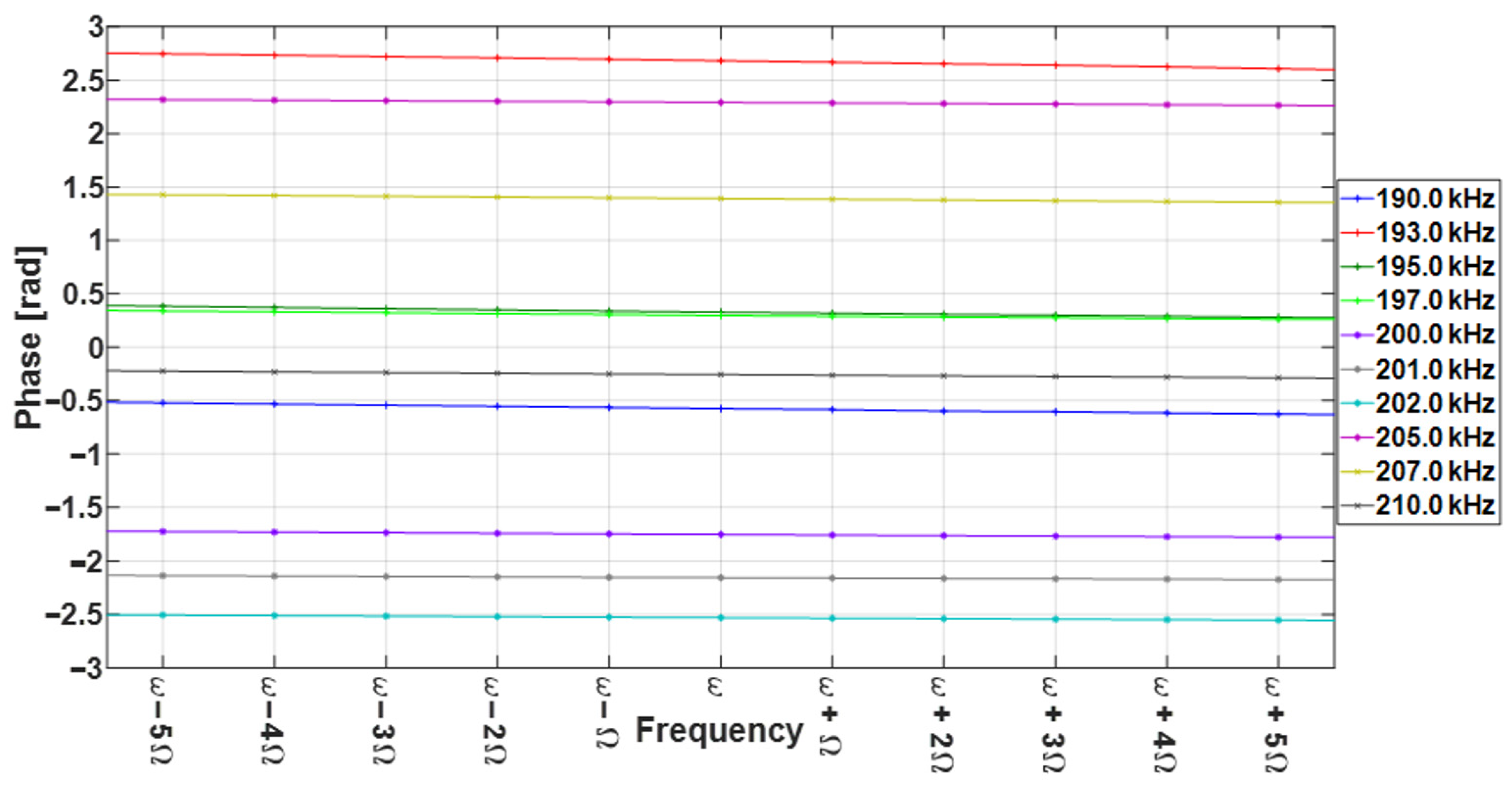
To compare the phase shift of an HF signal at sideband frequencies, a single-tone sinusoidal waveform at different frequencies was applied to a test sample, and the phase shift was calculated using the measured response at the receiver, as represented in Figure 8a. Figure 11 shows the measured HF response phase shifts at different frequencies. The frequency of the HF signal was selected equal to $\omega \pm k\mathsf{\Omega }$ for $k=0,1,2,\cdots$ to compare the phase shift at different sidebands’ frequencies.

$${{\phi }_4}_{\omega }={\theta }_{\omega }+{\theta }_{pz1}+{\theta }_{pz2}+{\theta }_{sp}$$

(13)

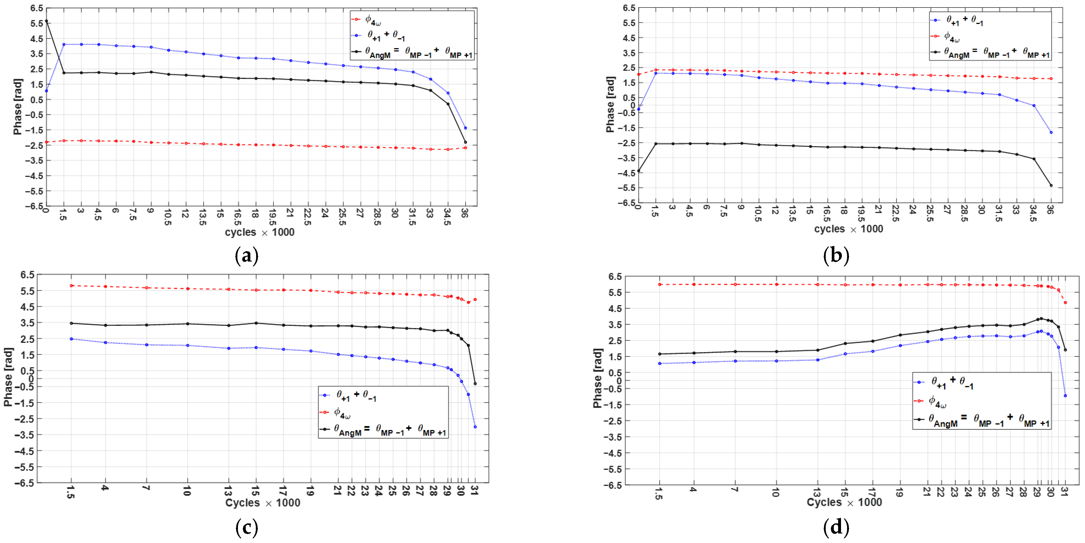
Results reveal that the phase shifts (${{\phi }_4}_{\omega })$ at $\omega \pm \mathsf{\Omega }$ and $\omega$ are almost equal, and the difference between phase shifts are negligible. Considering this finding, Equation (12) can be written as Equation (14). Finally, the value of the ${{\theta }_{MP}}_{+1}+{{\theta }_{MP}}_{-1}$, which is called angle modulation phase shift (${\theta }_{AngM}$), can be calculated using Equation (15). Figure 11 illustrates the results of the ${\theta }_{AngM}$ calculated at different frequencies.

$${\theta }_{+1}+{\theta }_{-1}=\left({{\phi }_4}_{\omega }\right)+\left({{\phi }_4}_{\omega }\right)+\left({{\theta }_{MP}}_{+1}+{{\theta }_{MP}}_{-1}\right)$$

(14)

$$\mathsf{\Phi }\left(m_a,m_f,m_p\right)\equiv {\theta }_{AngM}=\left({{\theta }_{MP}}_{+1}+{{\theta }_{MP}}_{-1}\right)=\left({\theta }_{+1}+{\theta }_{-1}\right)-2{{\phi }_4}_{\omega }$$

(15)

As evident in Figure 12, ${\theta }_{AngM}$ changes through the life cycle and reveals that phase shift changes with MIs. As noted earlier, the AFM model fails to explain the phase-shift variations associated with changes in MI. In contrast, the AFPM model successfully predicts these variations, which are also evident in experimental observations.

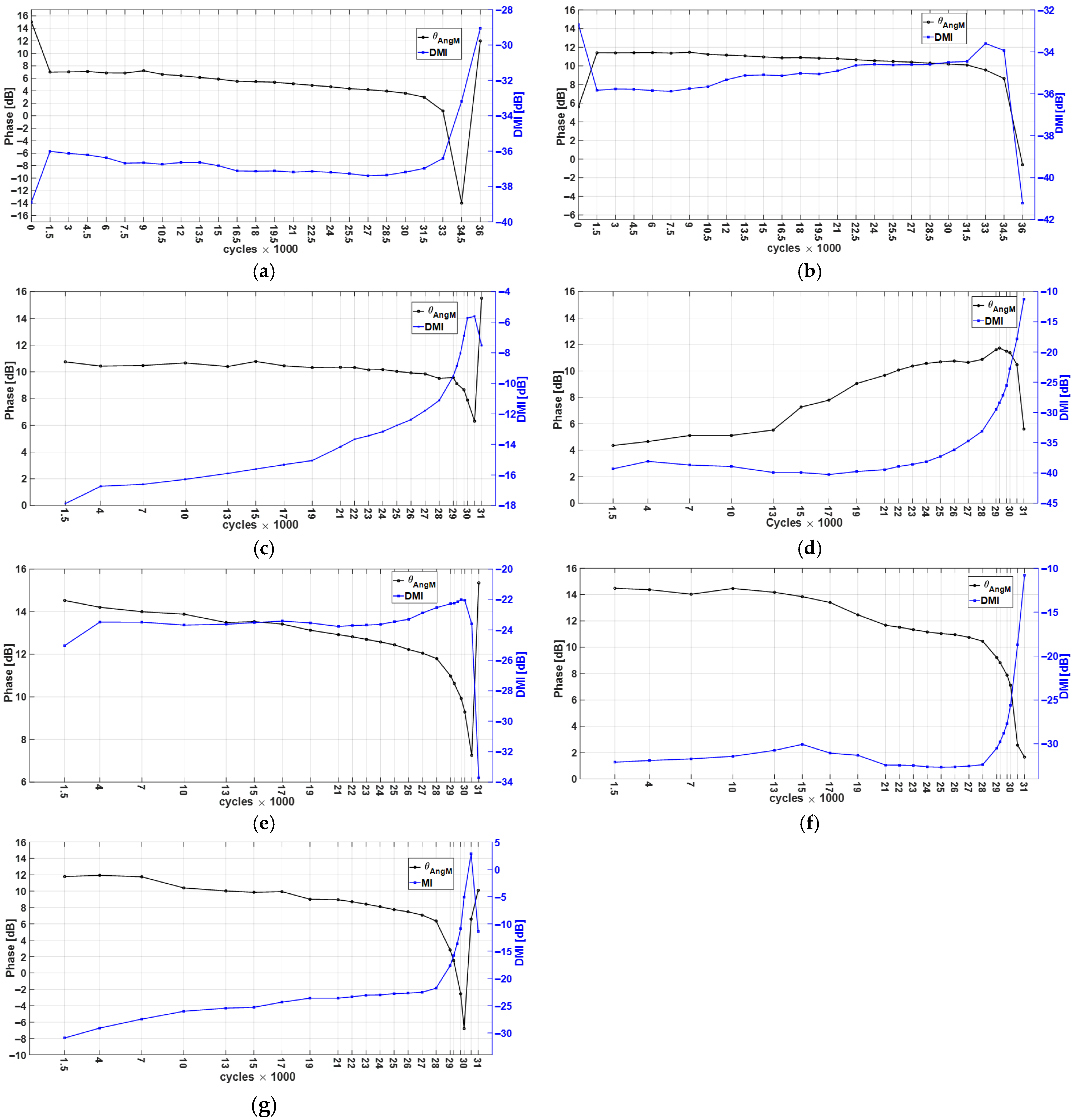
Figure 13 demonstrates that the angle-modulation phase shift, ${\theta }_{AngM}$, evolves consistently as the crack grows, confirming that phase information is fundamentally linked to the MIs, as predicted by the AFPM model. The measured ${\theta }_{AngM}$ provides direct experimental evidence that phase (PM) and frequency (FM) contributions coexist with amplitude modulation in the VAM response.

4. Discussion

The angle-modulation phase shift, ${\theta }_{AngM}$, and damage modulation index (DMI) curves obtained from the experimental results are analyzed to assess their potential for early defect detection.

Since specimens M6 and M14 failed after around 36,500 and 31,200 cycles, respectively, the relative lifetime of each specimen, expressed as a percentage of the total number of cycles at which measurements were performed, is shown in

Table 6. The details of the measured cycles for the M6 and M14 test setups.

M06	Cycle	0	1500	3000	4500	6000	7500	9000	10,500	12,000	13,500	15,000	16,500	18,000
	%	0	4%	8%	12%	16%	21%	25%	29%	33%	37%	41%	45%	49%
	Cycle	19,500	21,000	22,500	24,000	25,500	27,000	28,500	30,000	31,500	33,000	34,500	36,000
	%	53%	58%	62%	66%	70%	74%	78%	82%	86%	90%	95%	99%
M14	Cycle	1500	4000	7000	10,000	13,000	15,000	17,000	19,000	21,000	22,000	23,000	24,000	25,000
	%	5%	13%	22%	32%	42%	48%	54%	61%	67%	70%	74%	77%	80%
	Cycle	26,000	27,000	28,000	29,000	29,250	29,750	30,000	30,500	31,000
	%	83%	86%	90%	93%	94%	95%	96%	98%	99%

.

A direct comparison between the two curves is not feasible because their ranges of variation are not consistent. To eliminate this dimensional inconsistency and enable meaningful comparison, the data of both curves are normalized using Equation (16). Under the assumption that data (${\theta }_{AngM}$, DMI) at each frequency are independent of those at other frequencies, the minimum and maximum values for each frequency are used to normalize the data at that frequency.

$$x_{Norm}={\displaystyle \frac{x-min\left(x\right)}{max\left(x\right)-min\left(x\right)}}$$

(16)

After data normalization, the rate of change (slope) between successive points was calculated using three different approaches:

• Direct method: based on the normalized data.
• Mean–mean method: slope between the mean of several consecutive points and the mean of the preceding points.
• Point–mean method: slope between each point and the mean of its preceding points.

The slope variations of ${\theta }_{AngM}$ and DMI curves were compared across different frequencies and across all three calculation approaches for both the M6 and M14 test setups, as illustrated in

Table 7. The number of frequencies in M6 and M14 where the slope of variation in ${\theta }_{AngM}$ is bigger than DMI.

	Type of Evaluation	Lifetime	60% to 70%	70% to 80%	80% to 90%	60% to 75%	75% to 90%	60% to 80%	80% to 95%
M6	First method	N	7	9	6	5	3	5	4
		%	22.58%	29.03%	19.35%	16.13%	9.68%	16.13%	12.9%
	Second method	N	16	13	8	15	4	13	2
		%	51.61%	41.94%	25.81%	48.39%	12.9%	41.94%	6.45%
	Third method	N	28	28	24	28	24	28	15
		%	90.32%	90.32%	77.42%	90.32%	77.42%	90.32%	48.39%
M14	First method	N	21	22	20	18	16	12	10
		%	23.08%	24.18%	21.98%	19.78%	17.58%	13.19%	10.99%
	Second method	N	19	21	25	14	19	11	18
		%	20.88%	23.08%	27.47%	15.38%	20.88%	12.09%	19.78%
	Third method	N	40	47	37	40	34	38	26
		%	43.96%	51.65%	40.66%	43.96%	37.36%	41.76%	28.57%

. It should be noted that the total number of high frequencies measured at M6 and M14 test setups was 31 and 91, respectively.

The following conclusions can be drawn based on the results presented in Table 7:

• The above results clearly demonstrate that, at specific frequencies, the ${\theta }_{AngM}$ curve is capable of revealing larger variations than the MDI curve at earlier stages.
• It is worth noting that, as with the DMI curve, which at specific frequencies does not adequately reveal the nonlinearity of the specimen, the phase curve may also fail to reflect variations in response parameters, despite its theoretical higher sensitivity.
• These results should not be interpreted as evidence of the overall superiority of phase over the DMI. As illustrated in Figure 12 and summarized in Table 7, the DMI curve exhibits greater variations at specific frequencies. Nevertheless, the findings demonstrate that incorporating phase variation analysis can enhance the sensitivity to structural changes, often revealing variations more prominently than the amplitude-based approach.

5. Conclusions

After providing a literature review of current research on modulation index (MI) separation techniques, this article introduces an experimental study on damage detection in aluminum specimens using vibro-acoustic modulation (VAM). This study introduced a modulated response model combining all three types of modulation (amplitude, frequency, and phase), called the AFPM model. Unlike the amplitude–frequency modulation (AFM) model, the mathematical description of the AFPM reveals that phase shifts across frequency components are determined not only by the initial phase shifts of the low- and high-frequency signals, but also by changes in MIs. Additionally, relative sensitivity analysis of the damage modulation index (DMI) and angle modulation phase shift (${\theta }_{AngM}$) shows that ${\theta }_{AngM}$ is more sensitive than DMI and can be used for detecting defects at early stages.

The change in ${\theta }_{AngM}$ during a lifetime is tested experimentally, and evaluating the ${\theta }_{AngM}$ is explained step by step. Experimental results revealed that the ${\theta }_{AngM}$ vary over the lifetime of the samples, as predicted by the model. Additionally, the slope between successive points, calculated by normalized values of ${\theta }_{AngM}$ and DMI illustrated at specific frequencies, ${\theta }_{AngM}$ shows more change than MI in the early stages. The results demonstrate that combining phase and amplitude variation analysis can enhance sensitivity to structural changes, often revealing them more prominently than the amplitude-based approach alone, such as the DMI.

Nevertheless, selecting a parameter or set of parameters capable of accurately indicating the onset of crack initiation in the SUT requires comprehensive experimental investigations. Such studies should combine multiple defect-detection techniques and, in parallel, employ available technologies to assess the presence or absence of cracks at different scales (macro- or micro-levels). In addition, the results in Table 7 clearly show that the frequency selection (high and low) of the excitation signals plays a crucial role in the resulting performance. Optimally selecting a frequency when the crack location is unknown requires further investigation.

References

1. Donskoy, D.M.; Sutin, A.M. Vibro-Acoustic Modulation Nondestructive Evaluation Technique. J. Intell. Mater. Syst. Struct. 1998, 9, 765–771. [Google Scholar] [CrossRef] [Scilit]
2. Sutin, A.; Donskoy, D. Vibro-acoustic modulation nondestructive evaluation technique. In Proceedings of the Non-Destructive Evaluation Techniques for Aging Infrastructure and Manufacturing, San Antonio, TX, USA, 31 March–2 April 1998; SPIE: Bellingham, WA, USA, 1998; Volume 3397. [Google Scholar] [CrossRef] [Scilit]
3. Li, Z.; Wang, Z.; Xiao, L.; Qu, W. Damage detection and locating using tone burst and continuous excitation modulation method. In Proceedings of the SPIE Smart Structures and Materials + Nondestructive Evaluation and Health Monitoring, San Diego, CA, USA, 9–13 March 2014; SPIE: Bellingham, WA, USA, 2014; Volume 9064. [Google Scholar] [CrossRef] [Scilit]
4. Pieczonka, L.; Zietek, L.; Klepka, A.; Staszewski, W.; Aymerich, F.; Uhl, T. Damage imaging in composites using nonlinear vibro-acoustic wave modulations. Struct. Control Health Monit. 2018, 25, e2063. [Google Scholar] [CrossRef] [Scilit]
5. Xiao, C.; Zheng, H.; Hu, L.; Wang, Y.; Cao, Y. Study of micro-crack localization based on vibro-acoustic modulation. J. Phys. Conf. Ser. 2018, 1074, 012069. [Google Scholar] [CrossRef] [Scilit]
6. Aslam, M.; Bijudas, C.R.; Nagarajan, P.; Remanan, M. Numerical and Experimental Investigation of Nonlinear Lamb Wave Mixing at Low Frequency. J. Aerosp. Eng. 2020, 33, 04020037. [Google Scholar] [CrossRef] [Scilit]
7. Bazrafkan, M.M.; Rutner, M. Defect Localization in Metal Plates Using Vibroacoustic Modulation. NDT 2023, 1, 3–21. [Google Scholar] [CrossRef] [Scilit]
8. Klepkal, F.A.A.; Staszewski, W.J.; Uhl, T. Nonlinear vibro-acoustic wave modulations for impact damage detection in composites. In Proceedings of the 15th European Conference on Composite Materials, Venice, Italy, 24–28 June 2012. [Google Scholar]
9. Lim, H.J.; Sohn, H. Necessary Conditions for Nonlinear Ultrasonic Modulation Generation Given a Localized Fatigue Crack in a Plate-Like Structure. Materials 2017, 10, 248. [Google Scholar] [CrossRef] [Scilit] [PubMed]
10. Dorendorf, L.; Lalkovski, N.; Rutner, M. Physical explanation for vibro-acoustic modulation due to local and global nonlinearities in a structure and its experimental and numerical validation. J. Sound Vib. 2022, 528, 116885. [Google Scholar] [CrossRef] [Scilit]
11. Dorendorf, L.; Lalkovski, N.; Boll, B.; Rutner, M. Separation and quantification of damage-induced and non-damage-induced vibro-acoustic modulation and the problem of contrary modulations. Mech. Syst. Signal Process. 2025, 232, 112708. [Google Scholar] [CrossRef] [Scilit]
12. Boll, B.; Dorendorf, L.; Oppermann, P.; Willmann, E.; Fiedler, B.; Renner, B.-C.; Rutner, M.; Meißner, R.H. Synthetic generation of vibroacoustic modulation signals for structural health monitoring. Mech. Syst. Signal Process. 2023, 200, 110498. [Google Scholar] [CrossRef] [Scilit]
13. Donskoy, D.; Sutin, A.; Ekimov, A. Nonlinear acoustic interaction on contact interfaces and its use for nondestructive testing. NDT E Int. 2001, 34, 231–238. [Google Scholar] [CrossRef] [Scilit]
14. Duffour, P.; Morbidini, M.; Cawley, P. A study of the vibro-acoustic modulation technique for the detection of cracks in metals. J. Acoust. Soc. Am. 2006, 119, 1463–1475. [Google Scholar] [CrossRef] [Scilit]
15. Donskoy, D.M. Nonlinear Acoustic Methods. In Encyclopedia of Structural Health Monitoring; John Wiley & Sons, Ltd.: Hoboken, NJ, USA, 2009. [Google Scholar] [CrossRef] [Scilit]
16. Aymerich, F.; Staszewski, W.J. Experimental Study of Impact-Damage Detection in Composite Laminates using a Cross-Modulation Vibro-Acoustic Technique. Struct. Health Monit. 2010, 9, 541–553. [Google Scholar] [CrossRef] [Scilit]
17. Hu, H.F.; Staszewski, W.J.; Hu, N.Q.; Jenal, R.B.; Qin, G.J. Crack detection using nonlinear acoustics and piezoceramic transducers—Instantaneous amplitude and frequency analysis. Smart Mater. Struct. 2010, 19, 065017. [Google Scholar] [CrossRef] [Scilit]
18. Donskoy, D.M.; Ramezani, M. Separation of amplitude and frequency modulations in Vibro-Acoustic Modulation Nondestructive Testing Method. Proc. Meet. Acoust. 2018, 34, 045002. [Google Scholar] [CrossRef] [Scilit]
19. Donskoy, D.; Golchinfar, B.; Ramezani, M.; Rutner, M.; Hassiotis, S. Vibro-acoustic amplitude and frequency modulations during fatigue damage evolution. AIP Conf. Proc. 2019, 2102, 040004. [Google Scholar] [CrossRef] [Scilit]
20. Klepka, A.; Dziedziech, K.; Mrówka, J.; Górski, J. Experimental investigation of modulation effects for contact-type interfaces in vibro-acoustic modulation tests. Struct. Health Monit. 2021, 20, 917–930. [Google Scholar] [CrossRef] [Scilit]
21. Oppermann, P.; Dorendorf, L.; Rutner, M.; Renner, C. Nonlinear modulation with low-power sensor networks using undersampling. Struct. Health Monit. 2021, 20, 3252–3264. [Google Scholar] [CrossRef] [Scilit]
22. Gorski, J.; Dziedziech, K.; Klepka, A. Experimental investigation of modulation types in modulation transfer tests. Mech. Syst. Signal Process. 2023, 200, 110589. [Google Scholar] [CrossRef] [Scilit]
23. Klepka, A.; Staszewski, W.; Jenal, R.; Szwedo, M.; Iwaniec, J.; Uhl, T. Nonlinear acoustics for fatigue crack detection—Experimental investigations of vibro-acoustic wave modulations. Struct. Health Monit. 2012, 11, 197–211. [Google Scholar] [CrossRef] [Scilit]
24. Klepka, A.; Dziedziech, K. Vibro-acoustic modulation for damage detection -investigation of nonlinear effects for contact-type damage. In Proceedings of the International NDT Conference & Exhibition, Singapore, 27–28 February 2025. [Google Scholar] [CrossRef] [Scilit]
25. Haykin, S. Communication Systems, 4th ed.; Wiley India Pvt. Limited: Delhi, India, 2006. [Google Scholar]
26. Lathi, B.P.; Ding, Z. Modern Digital and Analog Communication Systems; Oxford University Press: Oxford, UK, 2010. [Google Scholar]
27. Donskoy, D.; Liu, D. Vibro-acoustic modulation baseline-free non-destructive testing. J. Sound Vib. 2021, 492, 115808. [Google Scholar] [CrossRef] [Scilit]
28. Donskoy, D.; Zagrai, A.; Chudnovsky, A.; Golovin, E.; Agarwala, V. Nonlinear vibro-acoustic modulation technique for life prediction of aging aircraft components. In Proceedings of the 3rd European Workshop—Structural Health Monitoring, Granada, Spain, 5–7 July 2006; Volume 2006, pp. 251–258. Available online: https://www.scopus.com/pages/publications/66749171931 (accessed on 5 January 2026).
Figure 1. The fundamentals of the Vibro-Acoustic Modulation method—(a) a test setup, (b) the frequency component of the response, when SUT has no defect, and (c) when SUT has a defect.
Ndt 04 00005 g001
Figure 2. The FFT spectrum of a simulated AFM signal using MATLAB 2024b: (a) the number of sidebands is theoretically infinite, and the phase shifts are 0 or π in the signals (see Table 1); (b) the phase shift of the signal components remains unchanged despite changes in the modulation indices (see Table 1).
Ndt 04 00005 g002
Figure 3. The FFT spectrum of a simulated AFPM signal using MATLAB: (a) the number of sidebands is theoretically infinite, and the phase shift of the signal components changes based on Table 3; (b) phase shifts of the signal components vary with the change in the MIs (see Table 3); (c) amplitudes and phase shifts are different when m a 2 = m a 1 , m f 2 = m p 1 and m p 2 = m f 1 ; (d) a 3D plot of the phase shift of the primary frequency component, θ 0 , when m a = 0.3 and m f and m p vary from 0 to 0.5 (see Table 3).
Ndt 04 00005 g003
Figure 4. The 3D plot of the phase shift at frequency ω , where the initial phase shifts are set to ϕ ω ,   ϕ = 0 ; (a) an AFM simulated signal; (b) an AFPM simulated signal for a constant m a = 0.02 .
Ndt 04 00005 g004
Figure 5. The 3D plot of the relative sensitivity (RS) of D M I m a , m f , m p and Φ m a , m f , m p evaluated in MATLAB 2024b, when (a) m a = 1 × 10 6 , (b) m a = 5 × 10 4 , and (c) m a = 1 × 10 3 .
Ndt 04 00005 g005
Figure 6. A general setup for the MI separation algorithm; (a) schematic sketch of the test setup; (b) an experimental setup.
Ndt 04 00005 g006
Figure 7. The LF load amplitude: (a) during the VAM measurement; (b) fatigue load.
Ndt 04 00005 g007
Figure 8. Frequency selection using the linear sweep; (a) linear sweep result for a test sample M6; (b) linear sweep result for a test sample M14; (c) FFT result of a chirp excitation for test sample MS5; (d) comparison between the chirp and single-tone excitation method results around an eigenfrequency at [60.8–60.9] kHz for the test sample MS5.
Ndt 04 00005 g008
Figure 9. The test setup for phase shifts measurement: (a) the VAM response setup; (b) the HF response setup.
Ndt 04 00005 g009aNdt 04 00005 g009b
Figure 10. The value of θ ω can be set to 0 by comparing the sent and measured response.
Ndt 04 00005 g010
Figure 11. The HF response phase shift ( φ 4 ) at different frequencies, ω ± ( k × 10 )   Hz for k = 0 , 1 , 2 , .
Ndt 04 00005 g011
Figure 12. Results of the calculated θ A n g M using Equation (15); (a) M6 test series, ω = 201.0   k H z ; (b) M6 test series, ω = 206.0   k H z ; (c) M14 test series, ω = 175.0   k H z ; (d) M14 test series, ω = 197.0   k H z .
Ndt 04 00005 g012
Figure 13. Comparison between the MI and θ A n g M ; (a) M6 test series, ω = 201.0   k H z ; (b) M6 test series, ω = 206.0   k H z ; (c) M14 test series, ω = 175.0   k H z ; (d) M14 test series, ω = 197.0   k H z ; (e) M14 test series, ω = 194.0   k H z ; (f) M14 test series, ω = 230.0   k H z ; (g) M14 test series, ω = 231.0   k H z .
Ndt 04 00005 g013