Abstract
This project assesses the feasibility of employing mobile air pollutant concentration monitoring along fixed routes within an urban community to evaluate near-road exposure. Continuous mobile air monitoring measurements of four pollutants (PM2.5, PM10, NO2, and O3) were collected using high-quality air monitors paired with a GPS device to track coordinates and vehicle speed. Simultaneous near-road measurements of the same pollutants were taken at two stationary sites to establish correlations with the mobile air monitoring data. The results indicate that pollutant concentrations recorded by mobile air monitors align closely with those from near-road stationary sites. This study demonstrated strong concordance between mobile and stationary monitoring for particulate matter concentrations, with PM2.5 and PM10 showing high correlation coefficients (R2 = 0.74 and 0.75, respectively). Ozone (O3) exhibited particularly consistent spatial distributions across all measurement platforms—mobile, near-road, and community stationary sites—as reflected in even stronger correlations (R2 = 0.93 and 0.89 for the two near-road sites). These robust associations suggest that mobile monitoring could serve as a viable alternative to stationary approaches for O3 assessment. In contrast, nitrogen dioxide (NO₂) measurements displayed greater variability, with mobile concentrations consistently exceeding near-road stationary values and demonstrating weaker correlation (R2 = 0.19), indicating potential limitations in mobile NO₂ monitoring reliability. This study highlights that mobile air pollutant monitoring in less congested communities can effectively capture exposure concentrations representative of both the community and near-road receptors represented by stationary air monitoring sites. Future research should explore how mobile air monitoring data can be utilized in exposure and health assessments, as well as how this technique can be applied in areas where stationary monitoring is impractical or prohibited due to cost or access limitations.
1. Introduction
Urban air pollution is a multifaceted challenge, with pollutant levels varying across space and time due to factors such as emission source locations and strengths, atmospheric chemical and photochemical processes, local and regional weather patterns, environmental topography, and prevailing background pollution levels. Transportation-related activities, especially those involving internal combustion engines, release a variety of harmful air pollutants that significantly impact public health and the environment. Exposure to these transportation-related air pollutants (TRAPs) can have detrimental effects on both human health and ecosystems. While individuals who exercise outdoors in polluted areas may face heightened health risks compared to those with less active lifestyles, the overall benefits of physical activity typically outweigh the negative effects of TRAP exposure [1,2,3,4]. Vulnerable population groups, such as children, elderly people, pregnant women, or people living in near-road communities, are especially susceptible to the TRAPs as reported in a number of epidemiological studies [5,6,7,8,9,10,11,12,13,14,15,16,17].
Quantifying the spatiotemporal changes in urban air pollution can lead to successful pollution control measures, lowering public exposure and related negative health consequences. Defining TRAPs necessitates extensive air pollution monitoring and a speciation network, which are costly, labor-intensive, and time-consuming. The data gathered might still be insufficient to conduct thorough effect assessments across wide study areas. To address the constraints of sparse stationary monitoring, mobile air pollution monitoring has been introduced. This strategy employs equipment mounted on movable platforms, such as vehicles, bicycles, or pedestrians, to provide continuous spatial records of pollution concentrations, resulting in a more dynamic and comprehensive dataset.
Because of its unique ability to assess instantaneously in both temporal and spatial dimensions, the fast-growing mobile air monitoring technique has established a firm foothold in air quality monitoring. Nonetheless, significant inherited difficulties remain to be addressed, particularly the link between its measurements and traditional time-averaged air quality data obtained at permanent stations. First, the spatial resolution of mobile measurements is a fundamental challenge in mobile sampling. Whether a sample represents an average concentration over a long road section or a point measurement separated by a specific distance needs to be addressed. The length of the road segment or the distance between two sampling points, or spatial resolution, depends on the vehicle speed and idle time. For instance, Shi et al. suggested an optimal spatial aggregation of 300 m based on their study in Hong Kong [18]. Second, the representativeness of a point measurement in space and time remains undefined. A point measurement collected along a long segment of a roadway could only represent an instantaneous observation of a three-dimensional concentration dataset that varies in space (first and second dimensions) and time (third dimension). Third, TRAPs decrease rapidly from highway to near-road locations. Karner et al. analyzed 41 roadside monitoring studies between 1978 and 2008 and concluded that almost all pollutants decay to background levels at a distance of 115 m to 570 m from the edge of the road, and the decay rate varies from one pollutant to another [19]. Venkatram et al. showed that the concentration of an inert pollutant decays rapidly to less than one fifth of its initial strength in 100 m in the direction normal to the roadway [20]. Thus, it is of paramount importance to understand the relationship between the data collected using the mobile technique and that reported from a nearby fixed station. Past literature has also explored both the benefits and limitations of mobile monitoring systems in enhancing community exposure assessments through the integration of stationary and mobile measurements. Castell et al. demonstrated the potential of combining mobile air monitoring technologies with environmental health monitoring to improve air quality data coverage in urban areas [21]. Similarly, Kousis et al. conducted a systematic literature review on urban mobile monitoring, identifying key challenges in this field—particularly methodological inconsistencies across studies that merge mobile and stationary data [22]. Despite these limitations, mobile monitoring stations offer a practical and efficient approach to collecting high spatial resolution data at varying aggregation levels within urban environments.
This project provides evidence for estimating near-road concentrations using transit vehicles traveling on fixed routes. Continuous mobile measurements of four pollutants (PM2.5, PM10, NO2, and O3) were recorded in conjunction with GPS locations. Concurrent near-road measurements were used to verify and provide associations with mobile data. The study tests two hypotheses: (1) community exposures to transportation pollutants can be represented by short-term spatio-temporal measurements using mobile air monitors; and (2) near-road receptors can be represented by mobile air monitors. The objectives of this study are to (1) provide reliable exposure concentration estimates for a community using transit vehicles equipped with mobile air monitors, and (2) evaluate associations of short-term TRAP concentrations with hourly exposure concentrations for near-road communities.
2. Materials and Methods
2.1. Study Area and Route Definition
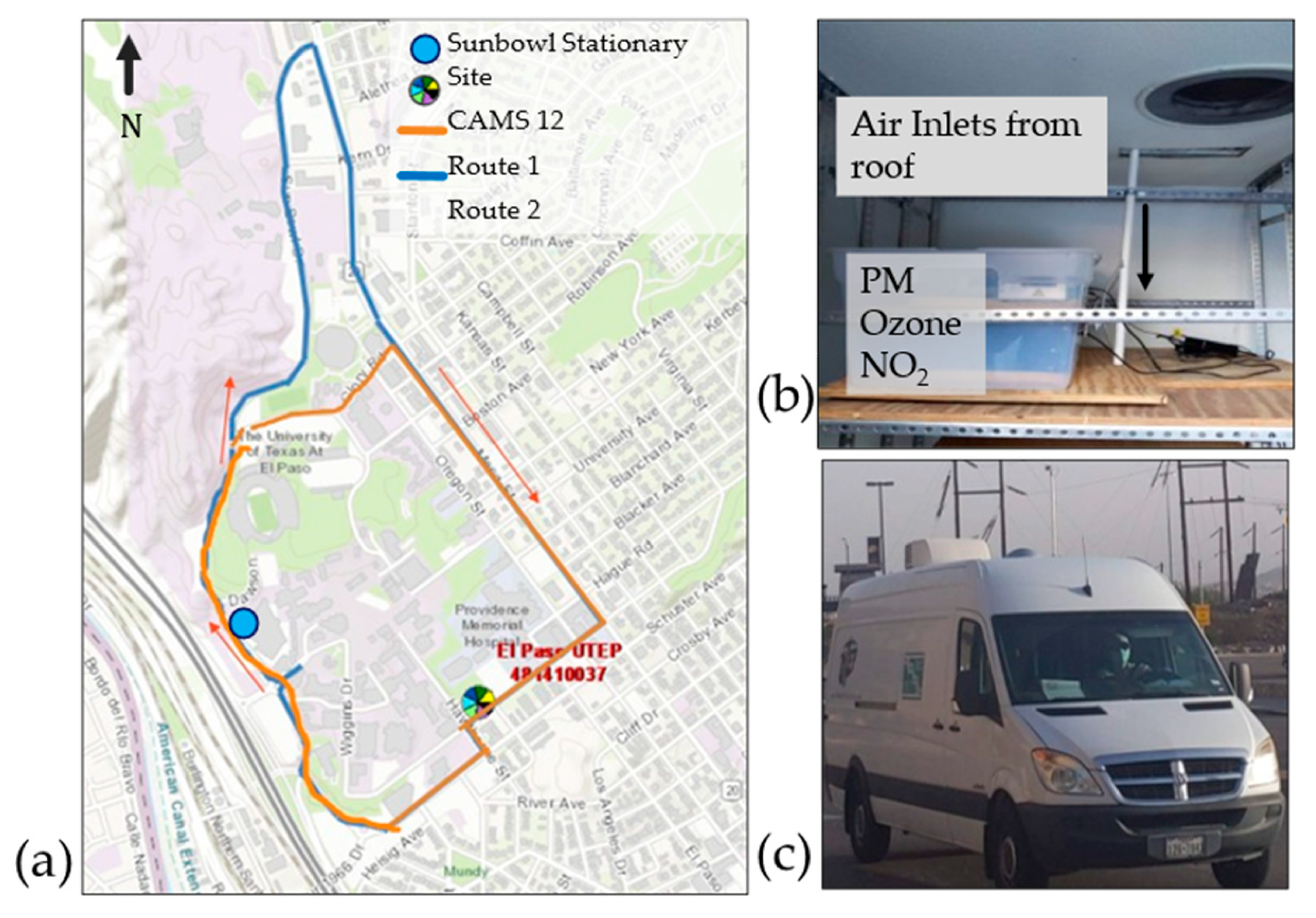
The study, conducted in El Paso, Texas, followed a route around the campus of the University of Texas at El Paso (UTEP). Mobile monitoring occurred along two designated routes in the community around the UTEP campus, as shown in Figure 1, with UTEP researchers driving at a speed of less than 30 miles per hour. The mobile monitoring routes in El Paso, Texas were strategically designed to capture pollution gradients across varying urban conditions: (1) high-traffic Mesa Street (AADT 25,000–35,000; 1–2 story buildings), (2) low-traffic Oregon Street (AADT 5000–8000; 1–2 story residential), and (3) transitional campus corridors (Sun Bowl Drive (AADT 16,000). The dual-loop design (inner campus perimeter and outer arterial extension) enabled sampling under prevailing WSW winds (3.5 m/s mean), with validation against the CAMS12 stationary site during stable meteorological conditions. This approach systematically assessed traffic intensity (12–35 k vehicles/day), building height (1–5 stories), and topographic (1140–1160 m elevation) influences on local air quality. The routes were designed to cover an arterial road (Mesa Street) with multiple traffic lights, a low traffic surface street (Oregon Street), and streets of different traffic intensity. The inner loop passes around the university campus, going from Sun Bowl Drive to Oregon Street and then onto Schuster Avenue (AADT 18,000). The outer loop extends to Sunbowl Drive so that it may go onto the higher traffic road, Mesa Street. Both routes stop at Schuster Avenue to bring the mobile monitoring facility closer to the first stationary site, CAMS12, also identified as El Paso UTEP C12/A125/X151/G125. This site is managed by the Texas Commission on Environmental Quality (TCEQ) and houses FRM/FEM data (according to U.S. EPA standards) that is then compared to air pollutant data obtained by the mobile monitoring station’s instruments. The second stationary site with identical air quality monitoring equipment was maintained on Sun Bowl Drive to offer additional data points for comparison. The stationary site monitoring locations, the mobile monitoring routes, and the details of the mobile monitoring platform are shown in Figure 1. The total length of the large loop (Route 1) is approximately 10 miles, and 8 miles for the smaller loop (Route 2), both of which are shown in Figure 1. Also shown in Figure 1 are the tube counter locations for counting arterial traffic on the route. Each trip lasted about 12–15 min and was conducted between 10 November and ended on 20 November 2020, during the entire work day. A total of 282 trips (170 outer loops and 112 inner loops) were conducted during this field study period, resulting in around 60 h of simultaneously collected data of PM2.5, PM10 O3, NO2, and GPS information. The traffic profile of the studied area exhibits distinct seasonal variations, with the selected study period reflecting a notably higher traffic volume compared to other times of the year. For instance, during summer months, vehicular activity near the university campus decreases significantly, whereas the fall semester coincides with peak traffic conditions. Consequently, this study focuses on evaluating air pollution levels through a combination of stationary and mobile measurements during a period characterized by maximal traffic density. This approach ensures that the findings are representative of the most congested traffic scenarios, thereby enhancing the generalizability of the results. The focus of this study was to evaluate the effectiveness of mobile monitors in estimating pollutant concentrations across various spatial areas by comparing the ambient pollutant concentrations measured by mobile monitors with those recorded by stationary monitors.

Figure 1.
(a) Study area and two mobile monitoring routes passing by stationary sites, CAMS 12 and Sunbowl, (b) inside view of the mobile monitoring platform including the three monitors and inlets, (c) overall view of the mobile monitoring platform.
2.2. Air and Traffic Pollutant Data Collection
Instrumentation and Setup
The UTEP air quality mobile van was set to accommodate the air monitoring equipment, which included an external air intake on the roof. In order to escape the upwind turbulence cavity zone that forms on the roof while the vehicle was in motion and to decrease the chance of cross-contamination of tailpipe emissions, the intake was positioned about 2 feet above the top of the mobile unit. Before the monitoring campaign, all air quality monitors were calibrated using data collected from the CAMS 12 site in a collocated configuration for 2 weeks [23].
Air quality data were collected by three different monitoring instruments. NO2 was measured using a 2B Technologies NO2/NO/NOx Monitor TM [24]. O3 was measured using a 2B Technologies Model 202 O3 Monitor [25]. Particulate matter was measured using a GRIMM Portable Laser Aerosol spectrometer and Dust Monitor [26]. The O3 and the NO2 instruments are U.S. EPA FEM-designated air monitors. Traffic data were collected at two points along the route shown in Figure 1. The TRAX Apollyon Counter/Classifier (JAMAR Technologies, 2010) collected vehicle volume counts for different vehicle types. Each counter included two tubes placed two feet apart; this method provided volume data and vehicle speed data for a two-way street. The vehicle volume was recorded for each hour of the day. The data were used for mobile emissions estimations using MOVES3, an EPA software; these data analyses and results are detailed in previous reports [23].
The configuration inside the mobile monitoring unit included one set of instruments with monitors placed on a shelving unit that helped reduce the vibration of the instruments during mobile monitoring. Inlet tubes were also shielded from rainwater. NO2 readings were collected every 10 s, O3 every 5 s, and PM2.5 and PM10 every 6 s. These intervals were the lowest allowed by each monitor. In order to collect longitude, latitude, and speed every second, a Columbus P-1 Professional GPS Data Logger was also placed with the air monitors. At the start of every day, the monitors were allowed to run for 30 min before beginning the mobile monitoring route to allow the monitors′ internal temperatures to stabilize so that readings could be the most accurate.
The stationary site at Sunbowl included the same set of instruments as those in the mobile monitoring unit. This site was established by the study, 5 m from the road, and collected continuous data every 5 min during the entire collection period. This station was only able to record NO2 and O3.
In this study, each 1 s of pollutant concentration mobile monitor measurement represents a spatial average over approximately 9–14 m of roadway when the vehicle was in motion, or <1 m when stationary. Each monitoring circuit required approximately 12 min to complete, yielding roughly 5 discrete data points per hour near stationary monitoring sites. These measurements enabled pseudo-collocated comparisons between mobile on-road concentrations and hourly averaged stationary site data.
To address spatial and temporal data sparsity while enhancing representativeness, mobile measurements were interpolated along extended roadway segments proximate to stationary monitors. Specifically, a 130 m roadway section was selected for comparisons with the Sunbowl stationary site, thereby improving statistical robustness through increased sampling density while maintaining spatial relevance to the reference monitor location.
Similarly, to compare the pollutant concentration data at the other stationary site, CAMS12, the mobile data collected at the 100 m by 100 m block (containing three stop-and-go traffic crossings) was averaged and compared to the recorded FRM data.
3. Results
3.1. Air Quality Data Results
3.1.1. Informative Statistics
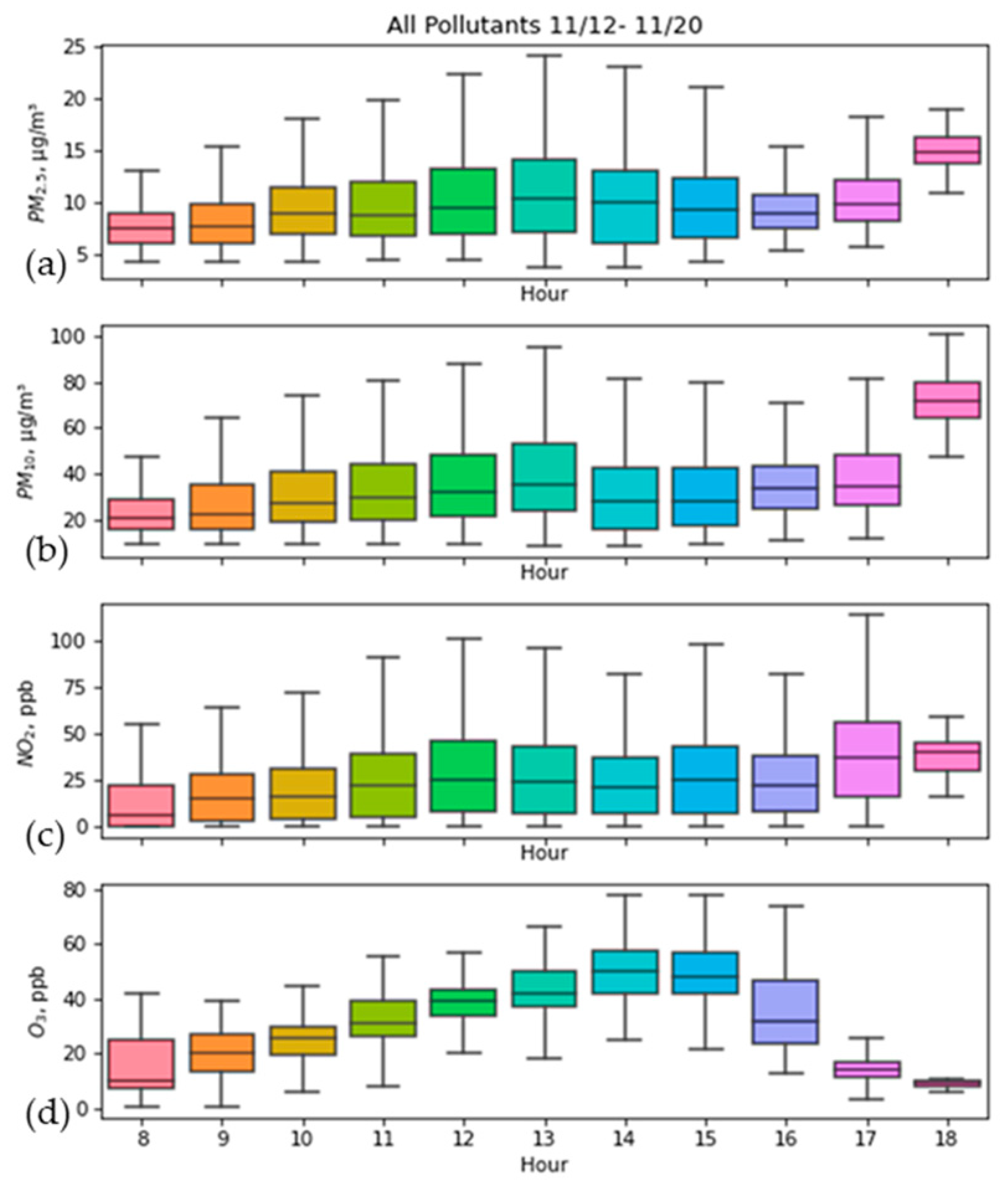
The diurnal trends of the pollutants assessed throughout the investigation are shown for all data gathered over the mobile monitoring period. Figure 2 shows a box plot of the hourly pollutant concentration along all routes throughout the study period, with the distribution of data for the hour labeled as minimum (Q1−1.5•IQR), first quartile (Q1), median, third quartile (Q3), and maximum (Q3+1.5•IQR).

Figure 2.
Hourly boxplot: pollutant data for all study period, (a) PM2.5, (b) PM10, (c) NO2, and (d) O3.
As predicted, the diurnal fluctuation of PM2.5 concentration is similar to that of PM10, with the overall average of PM2.5 concentration being around 30% of PM10. PM2.5 and PM10, both categories of particulate matter, frequently display analogous diurnal patterns due to their shared sources and atmospheric dynamics. PM10 encompasses particles with diameters up to 10 μm, whereas PM2.5 comprises particles with diameters up to 2.5 μm, making PM2.5 a subset of PM10. The diurnal variations in their concentrations are primarily driven by factors such as vehicular traffic, industrial emissions, and meteorological conditions [27]. PM10 levels average at 33.1 μg/m3, whereas PM2.5 levels average at 9.1 μg/m3. Particulate matter (PM) also peaks at about 12 p.m., which corresponds to usual lunchtime traffic patterns on campus. PM10 concentrations peak at approximately 75 µg/m3 at around 6 p.m., primarily due to elevated traffic volumes during this period. Furthermore, PM10 levels tend to rise after sundown during cooler months, driven by increased residential heating activities, including wood burning, which is prevalent along the U.S.–Mexico border in El Paso [28]. In El Paso, PM general peaks in the early morning hours around 6 a.m. and again in the early evening hours around 6 p.m. due to the traffic intensity, with the ratio for PM2.5 to PM10 being around 0.25 due to the high fugitive emissions from geologic sources, given that the area is surrounded by arid desert and traffic-enhanced emissions of road dust [29,30]. In El Paso, as in many other major cities, traffic increases in the early morning and late afternoon, resulting in the daily occurrence of PM peak. However, during the course of this investigation, traffic patterns in the study area deviated from the normal pattern of morning and evening peaks owing to the SARS-CoV2 epidemic.
The NO2 results in this research reveal a constant rise, with maximum values in the evening. NO2 is a main contaminant from emissions from tailpipes and a precursor in the O3-NO2 photolysis process. NO2 is rapidly depleted in the atmosphere during the day, particularly under high sun radiation, to create O3. When O3-NO2 photolysis stops working, NO2 begins to build after sunset. Meanwhile, O3 levels begin to climb in the morning when the sun rises, peak in the early afternoon when solar radiation is at its highest, and fall to a minimum after sunset. Figure 2c,d illustrates the O3-NO2 cycle for the Paso del Norte region. It also reveals that NO2 levels progressively grow in the morning, remain stable throughout the day, and begin to peak in the latter part of the day. The variance represents the balance between recurrent traffic emissions and NO2 photolysis throughout the daytime. As shown in the subsequent sections, O3 obtained by mobile monitoring has a good correlation with O3 measured at any nearby road site in the research region. This demonstrates the homogeneous distribution of O3 in the area, as opposed to the contemporary TCEQ data.
3.1.2. Spatio-Temporal Averages of Mobile Concentrations
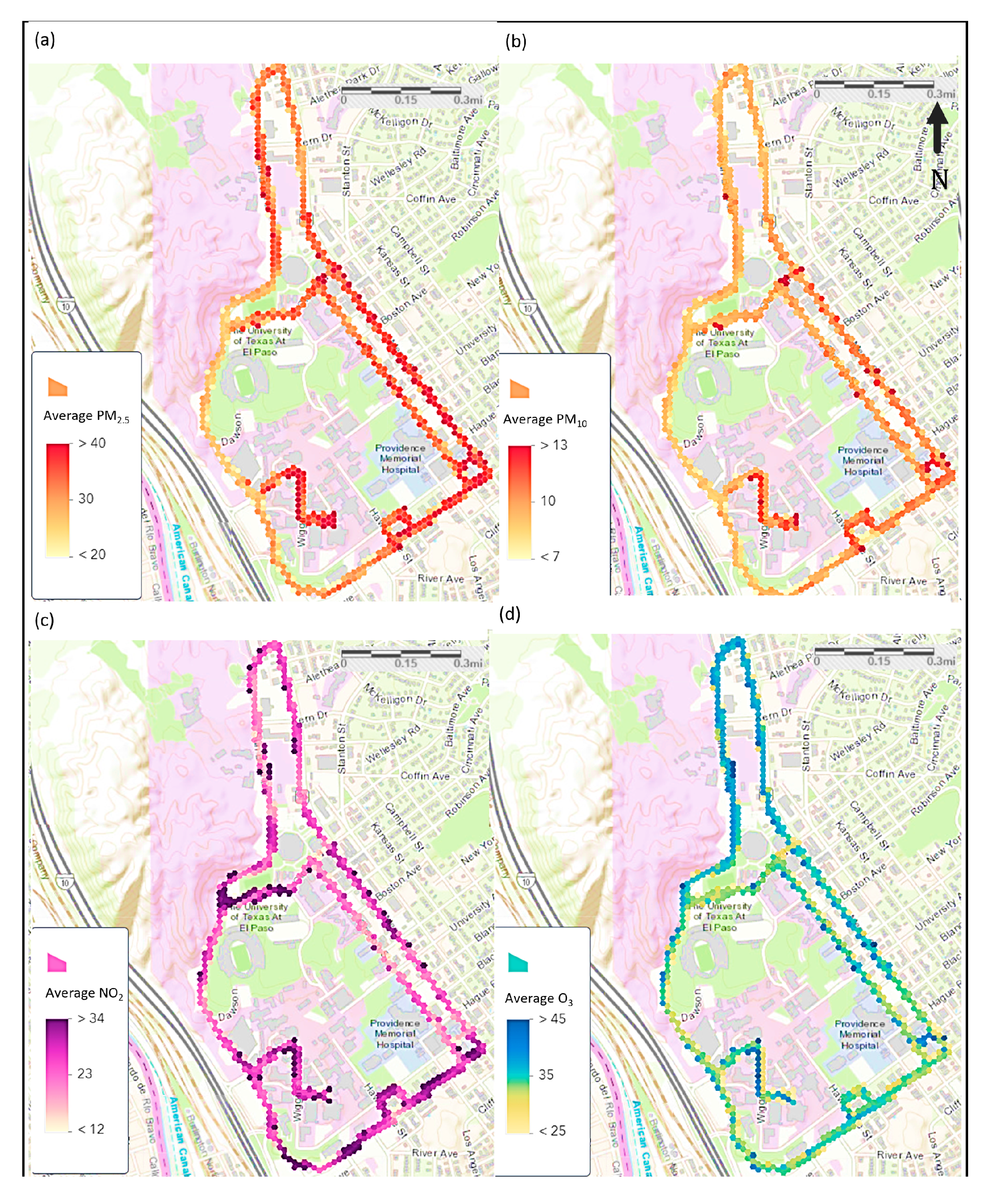
Figure 3 shows the hourly average of all pollutant values along the monitoring route. The 1 s data obtained from the mobile monitoring unit were averaged within 25 m hexagonal areas, averaged over all the days of the study. This graphic depicts hotspots at various areas throughout the research in a more generalized manner throughout the course of ten days. PM concentrations are greater in sections of the road with more junctions, whether free-flowing or stop-and-go. NO2 concentrations appear to spike at intersections and pauses along the mobile monitoring route. O3 follows a similar trend, peaking during slower parts of the route as well as stops and crossroads; however, it is the most common pollutant on the mobile monitoring route. It is clear that PM10 levels are highest near Mesa Street, the most crowded artery in the northwest half of the route, both throughout a 10-day period and on similar daily maps. PM2.5 levels peak in these places as well. Higher NO2 levels for the 10-day period are clustered and visible at the two roundabouts along the mobile monitoring route. This rise in NO2 might be ascribed to cars stopping and accelerating as they pass through the roundabout. As noted in the daily maps, O3 had an even distribution throughout the mobile monitoring route, with somewhat higher values when the vehicle was traveling at greater speeds, such as the stretch of Sunbowl as it approached the Mesa intersection. It is also worth noting how NO2 and O3 appeared to peak at opposing levels. Those areas along the mobile monitoring route with higher levels of NO2 correlate with those with significantly lower O3.
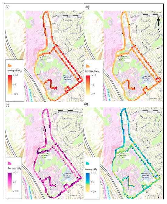
Figure 3.
All period average of mobile concentrations from 12 November to 20 November of 2020 for (a) PM2.5, (b) PM10, (c) NO2, and (d) O3.
3.1.3. Spatio Comparison of Near-Road Stationary and Mobile Measurements
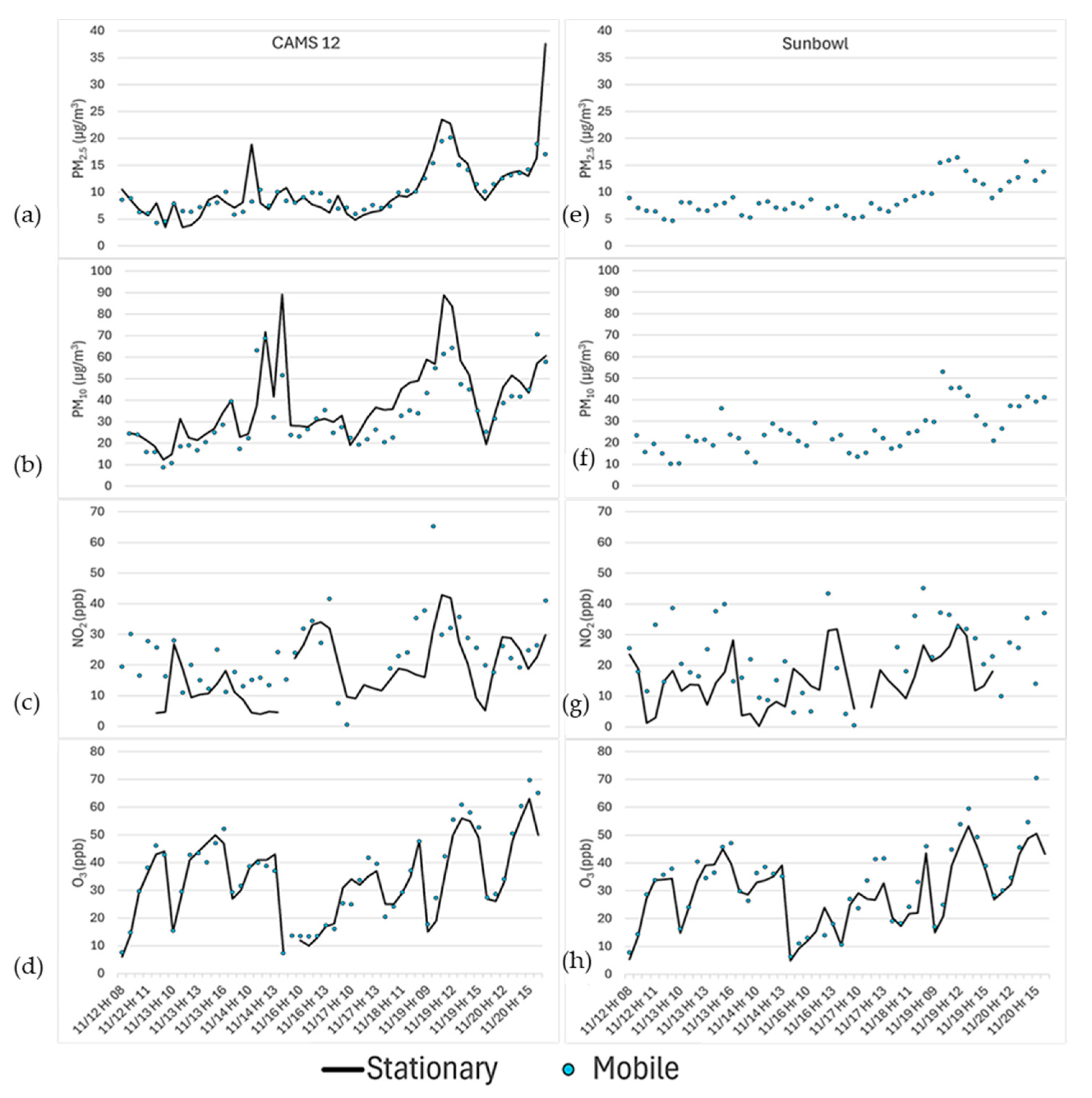
Mobile readings were matched to near-road measurements collected at two locations along the route. Because the mobile monitor was only positioned by the near-road sites for a few seconds at a time, and the near-road sites collect data by the hour, all instances of mobile readings by the near-road station during that hour were considered as the “mobile” measurement. Multiple drives along the route allowed for a higher density of mobile monitoring data points to be aggregated for the hourly comparison. In this study, we noticed that the mobile data have a significant correlation with fixed stationary site data. The near-road stationary locations varied between the sites, so that CAMS12 is around 40 m from the road, whereas the Sunbowl station is about 5 m from the road. This configuration is due to the nature of the sites. CAMS 12 is a state-operated site with its own siting requirements, and the Sunbowl station was established by this study as close as possible to the roadway. Figure 4 shows mobile measurements compared to the stationary measurements at CAMS 12 and Sunbowl. Data for PM at Sunbowl were not included due to instrument malfunction.
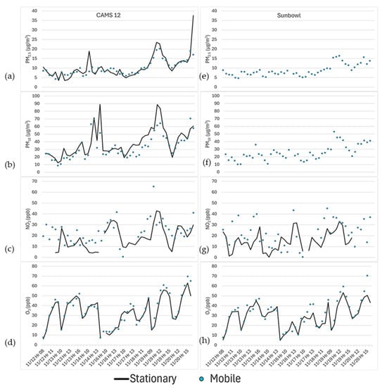
Figure 4.
Mobile monitoring and near-road stationary site pollutant levels at CAMS 12 (a) PM2.5, (b) PM10, (c) NO2, and (d) O3; and at Sunbowl, (e) PM2.5, (f) PM10, (g) NO2, and (h) O3.
PM10 and PM2.5 mobile readings and those taken at the near-road stationary site did not differ significantly at CAMS12, with PM10 levels higher than at the near-road stationary locations. Mobile NO2 values were comparable to near-road stationary site observations, but had greater peaks at both locations and were typically higher than those observed at the Sunbowl site. The differences in stationary NO2 and O3 concentrations at CAMS 12 compared to Sunbowl are most likely due to the amount of vehicle traffic surrounding each site. As mentioned previously, CAMS 12 is in closer proximity to roads with higher traffic volume (Schuster Ave, AADT 18,000). Mobile O3 values were nearly equal to those taken near the road at both sites. As prior investigations in this study have shown, O3 is widely distributed throughout the region and mostly fluctuates diurnally, but is ubiquitous over the spatial distribution. Further discussion on these relationships between the two modes of monitoring is presented in Section 4 below.
4. Discussion
4.1. Comparing Mobile and Stationary Data
Following data aggregation, the hourly mobile and stationary pollution statistics appear to agree quite well for all TRAPs on the road segments examined. The quick, complex photochemical reactions of NOx at the tailpipe may have led to the discrepancy between mobile and near-road stationary measurements. Nonetheless, the hourly averaged NO2 mobile data follows a similar trend and peaks at the same time as the data from this location. On average, mobile NO2 concentrations were 40% greater than those measured at fixed stations. Table 1 presents the correlation results between mobile and stationary data. For the stationary site providing PM data, CAMS 12, mobile monitoring concentrations were lower than those at the stationary site. This could imply that PM concentrations at this particular site were not influenced by transportation-related emissions. However, given that NO2 concentrations detected by the mobile monitor are 31% higher than the stationary site, CAMS 12, and 48% higher than the Sunbowl stationary site, it may be inferred that NO2 is a more reliable indicator of transportation-related emissions. Table 2 shows Pearson relationships and correlation coefficients for mobile and stationary data from both sites. Observing the Pearson connections between mobile and stationary data, it is clear that O3 has the strongest association between the two modes of measurement, with R2 values of 0.89 and 0.93 for Sunbowl and CAMS 12, respectively. Given this association, O3 may be efficiently monitored using mobile monitoring equipment instead of fixed monitoring equipment. PM2.5 and PM10 similarly had high R2 values (0.74 and 0.75, respectively). This location was 40 m from the road and at a higher elevation than the street where mobile monitoring occurred, which may explain the difference in mobile monitoring data and stationary data.

Table 1.
Period average pollutant concentrations for mobile and stationary monitors and the percent difference between mobile and stationary data.
Table 2.
Pearson correlation coefficients between mobile and stationary data at both sites, Sunbowl and CAMS 12.
The available hourly concurrent mobile and stationary pollution concentration data observed at the Sunbowl site are shown in Figure 4. Again, the mobile and stationary O3 data agree very well with each other, and the NO2 data deviate from each other at this site. The observed discrepancies between NO₂ concentrations at different monitoring sites, as well as the variations between mobile and stationary measurements, align with findings from prior studies. Brantley et al. (2014) demonstrated comparable variability in their mobile monitoring campaign, reporting significantly greater standard deviations for NO₂ concentrations across repeated sampling runs (inter-run variability) than those observed in hourly fluctuations at fixed sites [31]. This pattern suggests that spatial heterogeneity and transient emission sources contribute more substantially to NO₂ concentration variability than temporal factors alone in urban monitoring contexts. O3 data show excellent correlation between the two sets of data (Figure 4 and Table 1). NO2 data observed by the mobile monitor again show higher values than those observed at a roadside stationary site. Mobile NO2 concentrations are strongly affected by local meteorology, photolysis of NO2 and O3, solar radiation, and tailpipe emissions from various types of vehicles. Traffic density and vehicle speed at Sunbowl Drive were quite different from that of CAMS12, resulting in likely higher deviations of the TRAPs between the mobile data and the stationary roadside data.
4.2. Limitations and Applications
This study shows how to monitor TRAPs both mobile and stationary, utilizing high-quality air monitoring instruments and a GPS tracking device installed in the vehicle to give real-time data on pollutant concentrations, mobile measurement coordinates, and vehicle speed. The geographic resolution for each detected pollutant concentration relies on the monitor’s averaging time and vehicle speed. In this investigation, the minimum averaging periods for PM, NO2, and O3 monitors are 6, 5, and 10 s, respectively, resulting in minimum spatial averages of around 60 m, 100 m, and 50 m for each of the recorded mobile concentration data. The 1 s average concentrations between two continuous recorded measurements were estimated using interpolation to produce concentration data with a spatial average of roughly 10 m. The technique utilized in interpolation resulted in varying degrees of data smoothing, preventing monitors from detecting spatial change within the minimal detection zone. A monitoring device with a higher sampling frequency might assist in addressing this issue, especially if measurements are planned to take place on highways with higher speed limits where the mobile monitor will travel longer distances between measurements. It is difficult to quantify the impact of this limitation until further work is conducted with higher sampling frequency monitors. This study also concluded that mobile data may well represent the community exposure in a neighborhood where traffic emissions are less affected by the traffic and road conditions and where point sources are non-existent. Furthermore, the current study did not encounter any complicated emission conditions, such as cross-contamination from a vehicle’s own tailpipe emissions at traffic stops, traveling in the turbulent wake region behind a truck, being halted in traffic, traveling in roadways impacted by other point sources, or traveling in adverse weather conditions. These issues would have to be addressed, especially if a standard guideline for mobile monitoring were to be produced. Furthermore, this research was performed during the day, between 8 a.m. and 5 p.m. The data we have collected is not sufficient for making any conclusive comparison to 24 h averaged or longer-term averaged concentrations, which are needed for most air quality or health effect studies.
5. Conclusions
This project investigated the viability of utilizing mobile monitoring equipment traveling on defined routes to estimate near-road exposure levels. These exposure levels may help represent the exposure observed by communities participating in alternate modes of transportation. Continuous mobile readings of four TRAP (PM10, PM2.5, NO2, and O3) were collected together with GPS coordinates during various times of the day. Concurrent near-road measurements at a project-established stationary site, as well as a state-operated site monitoring data for the same pollutants, were used to validate and offer relationships with the mobile monitoring data.
In general, TRAP data collected by the mobile monitors is not significantly different from fixed stationary site data. Mobile NO2 measurements revealed significantly higher values than near-road stationary locations, particularly at a near-road site located approximately 40 m from the road and with an elevation difference of about 5 m. Mobile measurements compared to data acquired at the project-installed roadside stationary monitor (5 m away) revealed substantially more similar NO2 concentrations. Short-term spatiotemporal measurements with mobile air concentration monitors appear to be a potential way to reflect community exposure to traffic pollution. Spatiotemporal analysis revealed regions of concern for TRAPs without the necessity for several stationary locations. In general, near-road receptors can be represented by mobile air monitors. Further investigations are necessary into how mobile monitoring data can be utilized for exposure and health assessment, as well as how the technique can be used to quantify exposure concentrations in areas where stationary monitoring is not permitted or feasible due to cost or limitations of access.
Author Contributions
Conceptualization, M.C. and W.-W.L.; methodology, M.C. and W.-W.L.; validation, M.C., L.V.-R. and W.-W.L.; formal analysis, M.C. and W.-W.L.; investigation, M.C., L.V.-R. and E.W.; resources, W.-W.L.; writing—original draft preparation, M.C. and W.-W.L.; writing—review and editing, M.C. and W.-W.L.; visualization, M.C.; supervision, M.C. and W.-W.L.; project administration, W.-W.L.; funding acquisition, W.-W.L. All authors have read and agreed to the published version of the manuscript.
Funding
The contents of this report reflect the views of the authors, who are responsible for the facts and the accuracy of the information presented herein. This document is disseminated in the interest of information exchange. The report is funded, partially or entirely, by a grant from the U.S. Department of Transportation’s University Transportation Centers Program, Sponsoring Agent name and address U.S. Department of Transportation, 1200 New Jersey Avenue, SE, Washington, DC 20590; Grant Number 69A3551747119.
Institutional Review Board Statement
Not applicable.
Informed Consent Statement
Not applicable.
Data Availability Statement
Data available upon request.
Use of Artificial Intelligence
AI or AI-assisted tools were not used in drafting any aspect of this manuscript.
Acknowledgments
This research was supported, in whole or in part, by a grant from the U.S. Department of Transportation’s University Transportation Centers Program. The U.S. Government assumes no liability for the content or use of this report. The authors gratefully acknowledge this support and emphasize that the dissemination of this work is intended to advance knowledge and encourage further discussion in the field.
Conflicts of Interest
The authors declare no conflicts of interest.
References
- Aguilera, J.; Jeon, S.; Chavez, M.; Ibarra-Mejia, G.; Ferreira-Pinto, J.; Whigham, L.D.; Li, W.-W. Land-Use Regression of Long-Term Transportation Data on Metabolic Syndrome Risk Factors in Low-Income Communities. Transp. Res. Rec. 2021, 2675, 955–969. [Google Scholar] [CrossRef]
- Giles, L.V.; Koehle, M.S. The Health Effects of Exercising in Air Pollution. Sports Med. 2014, 44, 223–249. [Google Scholar] [CrossRef] [PubMed]
- Rundell, K.W.; Caviston, R. Ultrafine and Fine Particulate Matter Inhalation Decreases Exercise Performance in Healthy Subjects. J. Strength Cond. Res. 2008, 22, 2–5. [Google Scholar] [CrossRef] [PubMed]
- Cutrufello, P.T.; Smoliga, J.M.; Rundell, K.W. Small Things Make a Big Difference: Particulate Matter and Exercise. Sports Med. 2012, 42, 1041–1058. [Google Scholar] [CrossRef]
- Janssen, N.A.H.; Van Vliet, P.H.N.; Harssema, H.; Brunekreef, B. Assessment of Exposure to Traffic Related Air Pollution of Children Attending Schools near Motorways. Atmospheric Environ. 2001, 35, 3875–3884. [Google Scholar] [CrossRef]
- Spira-Cohen, A.; Chen, L.C.; Kendall, M.; Lall, R.; Thurston, G.D. Personal Exposures to Traffic-Related Air Pollution and Acute Respiratory Health Among Bronx Schoolchildren with Asthma. Environ. Health Perspect. 2011, 119, 559–565. [Google Scholar] [CrossRef]
- Kingsley, S.; Eliot, M.; Carlson, L.; Finn, J.; Macintosh, D.; Suh, H.; Wellenius, G. Proximity of US Schools to Major Roadways: A Nationwide Assessment. J. Expo. Sci. Environ. Epidemiol. 2014, 24, 253–259. [Google Scholar] [CrossRef]
- Iannuzzi, A.; Verga, M.C.; Renis, M.; Schiavo, A.; Salvatore, V.; Santoriello, C.; Pazzano, D.; Licenziati, M.R.; Polverino, M. Air Pollution and Carotid Arterial Stiffness in Children. Cardiol. Young 2010, 20, 186–190. [Google Scholar] [CrossRef]
- Armijos, R.X.; Weigel, M.M.; Myers, O.B.; Li, W.-W.; Racines, M.; Berwick, M. Residential Exposure to Urban Traffic Is Associated with Increased Carotid Intima-Media Thickness in Children. J. Environ. Public Health 2015, 2015, 713540. [Google Scholar] [CrossRef]
- Gilliland, F.D.; Berhane, K.; Rappaport, E.B.; Thomas, D.C.; Avol, E.; Gauderman, W.J.; London, S.J.; Margolis, H.G.; McConnell, R.; Islam, K.T.; et al. The Effects of Ambient Air Pollution on School Absenteeism Due to Respiratory Illnesses. Epidemiology 2001, 12, 43–54. [Google Scholar] [CrossRef]
- Chen, L.; Jennison, B.L.; Yang, W.; Omaye, S.T. Elementary School Absenteeism and Air Pollution. Inhal. Toxicol. 2000, 12, 997–1016. [Google Scholar] [CrossRef] [PubMed]
- Wendt, J.K.; Symanski, E.; Stock, T.H.; Chan, W.; Du, X.L. Association of Short-Term Increases in Ambient Air Pollution and Timing of Initial Asthma Diagnosis Among Medicaid-Enrolled Children in a Metropolitan Area. Environ. Res. 2014, 131, 50–58. [Google Scholar] [CrossRef] [PubMed]
- Barone-Adesi, F.; Dent, J.E.; Dajnak, D.; Beevers, S.; Anderson, H.R.; Kelly, F.J.; Cook, D.G.; Whincup, P.H. Long-Term Exposure to Primary Traffic Pollutants and Lung Function in Children: Cross-Sectional Study and Meta-Analysis. PLoS ONE 2015, 10, e0142565. [Google Scholar] [CrossRef] [PubMed]
- Gehring, U.; Cyrys, J.; Sedlmeir, G.; Brunekreef, B.; Bellander, T.; Fischer, P.; Bauer, C.P.; Reinhardt, D.; Wichmann, H.E.; Heinrich, J. Traffic-Related Air Pollution and Respiratory Health During the First 2 Yrs of Life. Eur. Respir. J. 2002, 19, 690–698. [Google Scholar] [CrossRef]
- Ierodiakonou, D.; Zanobetti, A.; Coull, B.A.; Melly, S.; Postma, D.S.; Boezen, H.M.; Vonk, J.M.; Williams, P.V.; Shapiro, G.G.; McKone, E.F.; et al. Ambient Air Pollution, Lung Function, and Airway Responsiveness in Asthmatic Children. J. Allergy Clin. Immunol. 2016, 137, 390–399. [Google Scholar] [CrossRef]
- Forns Guzman, J.; Dadvand, P.; Foraster, M.; Alvarez-Pedrerol, M.; Rivas, I.; López-Vicente, M.; Suades González, E.; García-Esteban, R.; Esnaola, M.; Cirach, M.; et al. Traffic-Related Air Pollution, Noise at School, and Behavioral Problems in Barcelona Schoolchildren: A Cross-Sectional Study. Environ. Health Perspect. 2015, 124, 529–535. [Google Scholar] [CrossRef]
- Lovinsky-Desir, S.; Jung, K.H.; Montilla, M.; Quinn, J.; Cahill, J.; Sheehan, D.; Perera, F.; Chillrud, S.N.; Goldsmith, J.; Perzanowski, M.; et al. Locations of Adolescent Physical Activity in an Urban Environment and Their Associations with Air Pollution and Lung Function. Ann. Am. Thorac. Soc. 2021, 18, 84–92. [Google Scholar] [CrossRef]
- Shi, Y.; Lau, K.K.-L.; Ng, E. Developing Street-Level PM2.5 and PM10 Land Use Regression Models in High-Density Hong Kong with Urban Morphological Factors. Environ. Sci. Technol. 2016, 50, 8178–8187. [Google Scholar] [CrossRef]
- Karner, A.A.; Eisinger, D.S.; Niemeier, D.A. Near-Roadway Air Quality: Synthesizing the Findings from Real-World Data. Environ. Sci. Technol. 2010, 44, 5334–5344. [Google Scholar] [CrossRef]
- Venkatram, A.; Snyder, M.; Isakov, V.; Kimbrough, S. Impact of Wind Direction on Near-Road Pollutant Concentrations. Atmos. Environ. 2013, 80, 248–258. [Google Scholar] [CrossRef]
- Castell, N.; Kobernus, M.; Liu, H.-Y.; Schneider, P.; Lahoz, W.; Berre, A.J.; Noll, J. Mobile Technologies and Services for Environmental Monitoring: The Citi-Sense-MOB Approach. Urban. Clim. 2015, 14, 370–382. [Google Scholar] [CrossRef]
- Kousis, I.; Manni, M.; Pisello, A.L. Environmental Mobile Monitoring of Urban Microclimates: A Review. Renew. Sustain. Energy Rev. 2022, 169, 112847. [Google Scholar] [CrossRef]
- Chavez, M.C.; Li, W.W.; Williams, E.; Vazquez, L. Using Transit Vehicles as Probes to Monitor Community Air Quality and Exposure; Center for Transportation, Environment, and Community Health: Ithaca, NY, USA, 2021. [Google Scholar]
- 2B Technologies. NO2/NO/NOx Monitor Operation Manual; 2B Technologies: Broomfield, CO, USA, 2017. [Google Scholar]
- 2B Technologies. Ozone Monitor Operation Manual; 2B Technologies: Broomfield, CO, USA, 2017. [Google Scholar]
- GRIMM. Specification for Portable Laser Aerosol Spectrometer and Dust Monitor Model 1.108/1.109. In Users Manual; GRIMM Aerosol: Ainring, Germany, 2010. [Google Scholar]
- Cholianawati, N.; Sinatra, T.; Nugroho, G.A.; Agustian Permadi, D.; Indrawati, A.; Halimurrahman; Kallista, M.; Romadhon, M.S.; Ma’ruf, I.F.; Udhatama, D.; et al. Diurnal and Daily Variations of PM2.5 and Its Multiple-Wavelet Coherence with Meteorological Variables in Indonesia. Aerosol. Air Qual. Res. 2024, 24, 230158. [Google Scholar] [CrossRef]
- Comrie, A.C. An All-Season Synoptic Climatology of Air Pollution in the U.S.-Mexico Border Region∗. Prof. Geogr. 1996, 48, 237–251. [Google Scholar] [CrossRef]
- Li, W.W.; Orquiz, R.; Garcia, J.H.; Espino, T.T.; Pingitore, N.E.; Gardea-Torresdey, J.; Chow, J.; Watson, J.G. Analysis of Temporal and Spatial Dichotomous PM Air Samples in the El Paso-Cd. Juarez Air Quality Basin. J. Air Waste Manag. Assoc. 2001, 51, 1551–1560. [Google Scholar] [CrossRef]
- García, J.H.; Li, W.W.; Arimoto, R.; Okrasinski, R.; Greenlee, J.; Walton, J.; Schloesslin, C.; Sage, S. Characterization and Implication of Potential Fugitive Dust Sources in the Paso del Norte Region. Sci. Total Environ. 2004, 325, 95–112. [Google Scholar] [CrossRef]
- Brantley, H.L.; Hagler, G.S.W.; Kimbrough, E.S.; Williams, R.W.; Mukerjee, S.; Neas, L.M. Mobile Air Monitoring Data-Processing Strategies and Effects on Spatial Air Pollution Trends. Atmos. Meas. Tech. 2014, 7, 2169–2183. [Google Scholar] [CrossRef]
Disclaimer/Publisher’s Note: The statements, opinions and data contained in all publications are solely those of the individual author(s) and contributor(s) and not of MDPI and/or the editor(s). MDPI and/or the editor(s) disclaim responsibility for any injury to people or property resulting from any ideas, methods, instructions or products referred to in the content. |
© 2025 by the authors. Licensee MDPI, Basel, Switzerland. This article is an open access article distributed under the terms and conditions of the Creative Commons Attribution (CC BY) license (https://creativecommons.org/licenses/by/4.0/).