Article

Association Analysis of Benzo[a]pyrene Concentration Using an Association Rule Algorithm

Graduate School of Energy Science, Kyoto University, Kyoto 606-8501, Japan
*
Author to whom correspondence should be addressed.
Submission received: 6 March 2025 / Revised: 7 May 2025 / Accepted: 8 May 2025 / Published: 12 May 2025

Abstract

:
Benzo[a]pyrene is an important indicator of polycyclic aromatic hydrocarbons pollution that exhibits complex atmospheric dynamics influenced by meteorological factors and suspended particulate matter (SPM). Herein, the factors influencing B(a)P concentration were elucidated by analyzing the monthly environmental data for Kyoto, Japan, from 2001 to 2021 using an improved association rule algorithm. Results revealed that B(a)P concentrations were 1.3–3 times higher in cold seasons than in warm seasons and SPM concentrations were lower in cold seasons. The clustering performance was enhanced by optimizing the K-means method using the sum of squared error. The efficiency and reliability of the traditional Apriori algorithm were enhanced by restructuring its candidate itemset generation process, specifically by (1) generating C2 exclusively from frequent itemset L₁ to avoid redundant database scans and (2) implementing the iterative pruning of nonfrequent subsets during Lk → Ck+1 transitions, adding the lift parameter, and eliminating invalid rules. Strong association rules revealed that B(a)P concentrations ≤ 0.185 ng/m3 were associated with specific meteorological conditions, including humidity ≤ 58%, wind speed ≥ 2 m/s, temperature ≥ 12.3 °C, and pressure ≤ 1009.2 hPa. Among these, changes in pressure had the most substantial impact on the confidence of the association rules, followed by humidity, wind speed, and temperature. Under the influence of high SPM concentrations, favorable meteorological conditions further accelerated pollutant dispersion. B(a)P concentration increased with increasing pressure, decreasing temperature, and decreasing wind speed. Principal component analysis confirmed the robustness and accuracy of our optimized association rule approach in quantifying complex, nonlinear relationships, while providing granular, interpretable insights beyond the traditional methods.

1. Introduction

Polycyclic aromatic hydrocarbons (PAHs) are organic environmental pollutants that pose significant risks to human health and the environment [1,2]. They exhibit strong hematotoxic, mutagenic, carcinogenic, and immunosuppressive effects and cause irreparable damage upon binding with DNA or RNA [3,4]. The U.S. Environmental Protection Agency (USEPA) has listed 16 PAHs as priority pollutants, including benzo[a]pyrene (B(a)P) as an IARC Group I human carcinogen [5,6]. B(a)P, a representative carcinogenic substance, is considered an important indicator of the health hazard load posed by PAHs. The carcinogenic activity of PAHs mixtures adsorbed on particulate matter has consistently contributed to their overall toxicity [7]. Since B(a)P has low volatility in atmospheric media, the majority of it is distributed in the particle phase, particularly as fine particles such as PM2.5.
The sources, transportation, transformation, and interactions of PAHs with atmospheric pollutants under various influencing conditions have been elucidated using different analytical methods [8,9]. Although conventional pollutant monitoring primarily relies on fixed stations and offline analyses, recent advancements in mobile sensing networks have enabled the dynamic tracking of pollutant variations. For instance, Lotrecchianoa et al. [10] developed a real-time on-road monitoring system that captures transient pollution events and provides high-resolution spatio-temporal data. This approach addresses the spatial coverage limitations of static stations and offers opportunities for integrating real-time streaming data with machine learning models. The correlation between atmospheric pollutants and meteorological conditions [11,12] has also been elucidated using statistical analysis, numerical simulation, and machine learning [13,14,15]. Meteorological factors, such as pressure, humidity, wind speed, and temperature, considerably influence variations in B(a)P concentrations. These factors affect the formation, dispersion, and deposition of suspended particulate matter (SPM), which in turn indirectly or directly affects B(a)P concentration.
Statistical methods such as linear regression, time series analysis, and principal component analysis (PCA) qualitatively analyze the correlation between two factors using correlation coefficients that directly represent the positive or negative influence of variable X on outcome Y. For instance, periodic canonical correlation analysis was used to analyze the strong correlation between the measured Stokes data and the reference concentrations of five components in SPM, namely, Si, K, Fe, Ca, and Zn [16]. Dust deposition in Africa from 1980 to 2018 was studied via remote sensing and correlation analysis, which revealed that the relation between PM2.5 and multispectral carbon monoxide (CO) from abundant atmospheric pollutants in Central Africa varied across different months [17]. The impact of three meteorological conditions on atmospheric PM concentrations in Rome, Italy, during the winter of 2017 was investigated via statistical analysis. Results revealed that, except on rainy days, the optimal conditions for PM dispersion were provided when the north wind exceeded 4 m/s and persisted for at least 24 h [18].
However, statistical methods are primarily employed to analyze qualitative and semiquantitative relationships between factors and often cannot quantitatively capture complex nonlinear interactions among multiple factors. Therefore, numerical simulation models, such as the community multiscale air quality model (CMAQ) and the weather research and forecasting model coupled with CMAQ (WRF-Chem), are used to simulate the distribution, transmission, and transformation of atmospheric pollutants [19,20]. During simulation, extensive data are collected from the study area, which include topographical data (surface height and type); land use information (urban and industrial spatial distribution); various emission sources (point sources, line sources, and area sources); meteorological factors (solar radiation, precipitation, and temperature); and boundary conditions (atmospheric background concentration and initial concentration distribution). As the majority of data are not physically available due to issues, such as resolution, idealized data or data interpolation and model generation techniques are used. Parameters for the atmospheric boundary layer and information on the emission heights of pollution sources are also uncertain. Therefore, simulated and actual pollutant concentrations show discrepancies [21,22].
Conventional methods such as statistical analysis and numerical simulations do not meet the requirements for high processing efficiency and accuracy. Therefore, machine learning algorithms are combined to rapidly and precisely identify patterns from large datasets. Furthermore, mobile sensor networks offer significant advantages for machine learning algorithms. As demonstrated by Lotrecchianoa et al. [10], continuous data streams from on-road sensors enable the adaptive training of models such as random forests, improving their accuracy in predicting PM2.5-B(a)P correlations under dynamic meteorological conditions. For instance, hourly ozone concentrations in Thessaloniki, Greece, were predicted using a backpropagation (BP) neural network [23]. Results revealed that machine learning algorithms are reliable and accurate for the time series simulation of air pollution. Moreover, machine learning algorithms, including K-means clustering and Pearson correlation coefficient, have been used to determine the relationship between high daily PM10 concentrations and meteorological factors [24]. Machine learning algorithms such as support vector machines, artificial neural networks, and random forests are used to predict the relationship between various air pollutants and meteorological variables [25], proving that they can facilitate better pollution prevention and control.
Herein, we employ data mining techniques within the machine learning framework to investigate the key factors influencing atmospheric B(a)P concentrations and their nonlinear relationships. In particular, we quantitatively examine the synergistic effects of meteorological factors—such as humidity, wind speed, temperature, and atmospheric pressure—and SPM on variations in B(a)P concentrations.
To address the limitations of conventional methods in capturing complex atmospheric interactions, we propose a dual-innovation framework as follows:
  • Algorithmically Enhanced Apriori Mining:
We re-engineered the classical Apriori framework to achieve enhanced efficiency through the following strategies:
(i)
Pruned database scanning: Candidate sets are iteratively generated from previous frequent itemsets (eliminating redundant full-database scans).
(ii)
Lift-based statistical filtering (lift ≥ 3.0): Minimally sufficient rules are retained only if dimensional expansion does not alter confidence or lift metrics.
(iii)
Dimensionality-aware optimization: Minimally sufficient rules are preserved during dimensional expansion.
2.
Hybrid Analytical Architecture:
We developed a novel integration of SSE-optimized K-means clustering (for precise cluster identification), enhanced association rule mining, and nonlinear PCA validation to uniquely resolve linear (via PCA) and nonlinear (via association rules) interactions in atmospheric systems—overcoming the single-model limitations of previous studies.
This approach provides a multimodal methodology for evaluating pollutant variations under multifactorial influences. To this end, data from multiple air quality monitoring stations in Kyoto Prefecture, Japan, were collected from January 2001 to December 2021. Using the proposed framework, the variation in B(a)P concentration under the combined influence of SPM and meteorological factors was quantitatively analyzed, and the sensitivity ranking of meteorological drivers was systematically derived.

2. Materials and Methods

2.1. Data Collection and Analysis

Environmental monitoring data—B(a)P, SPM, and meteorological data—from four cities (Kyoto, Yawata, Fukuchiyama, and Uji); five wards in Kyoto City (Kita, Nakagyo, Ukyo, Sakyo, and Yamashina); and two towns (Kumiyama and Oyamazaki) within Kyoto Prefecture over January 2001–December 2021 were obtained from the public platforms of the National Institute for Environmental Studies (NIES) (https://tenbou.nies.go.jp/) (accessed on 6 June 2024) and the Japan Meteorological Agency (JMA) (https://www.data.jma.go.jp/stats/etrn/index.php) (accessed on 6 June 2024). The geospatial boundaries of administrative units (cities and towns) were derived from the digital map database provided by the Geospatial Information Authority of Japan (GSI) (https://www.gsi.go.jp/gis.html) (accessed on 7 May 2025) in Figure 1. SPM refers to airborne particles with an aerodynamic diameter of ≤10 µm. SPM is predominantly used in Japan for air quality monitoring and regulation.
All SPM and B(a)P measurements were conducted monthly at the same monitoring stations using high-volume (Hi-Vol) or low-volume (Lo-Vol) air samplers. Particulate matter was collected on quartz fiber filters without size-selective inlets, ensuring the capture of total suspended particulate matter. B(a)P extraction followed standardized protocols: filters were sonicated in dichloromethane, purified using silica gel column chromatography, and quantified by GC–MS using a capillary column and SIM mode. Meteorological factors, including wind speed, wind direction, temperature, humidity, and atmospheric pressure, were primarily recorded using standard meteorological instruments installed at these stations. In cases where meteorological instruments were unavailable at the same location, data from nearby meteorological stations were used as substitutes. All collected data were preprocessed to eliminate invalid or erroneous values and address missing data where necessary. The B(a)P dataset was complete across all regions, with no missing data points.

2.2. Data Discretization

Numerical data stored after quality control must undergo discretization for use in association rule algorithms. K-means clustering was used to divide different data types into distinct intervals and assign specific symbols to represent raw data. K-means clustering fundamentally computes the distance D between each data point and the predefined centroids [26,27,28]. A smaller distance D implies a stronger correlation among the data.
To reduce the number of iterative experiments, an elbow method metric (i.e., the sum of squared error [SSE]) was introduced into the original algorithm to represent the size of clustering errors, as detailed in Appendix A.1 [29,30].
A Python-based program (Python 3.7.7; PyCharm Community 2020.1, JetBrains) was developed to perform clustering on various data based on the SSE principle. Figure 2 shows the elbow plot representing the optimal K values. Based on the inflection points of data and the original data properties, K = 3 was deemed the best clustering configuration. The factors were categorized into three intervals—low, medium, and high. As shown in Figure 2, when K = 4, the SSE value is the lowest. However, upon dividing the data into four categories (the values of data are from low to high), substantial differences were observed in the distribution of data across intervals, resulting in a classification outcome that could provide insufficient quality for subsequent association rule mining. Table 1 shows the final grading, where B, SP, T, H, and P denote the B(a)P concentration (ng/m3), SPM concentration (mg/m3), wind speed (m/s), temperature (°C), H humidity (%), and pressure (hPa), respectively. Table 2 shows the results of data mining. Wind direction was excluded herein due to its considerable temporal variations.

2.3. Optimization of Association Rule Algorithm

By employing association rule learning in unsupervised machine learning algorithms, a series of strong association rules can be derived by identifying and compressing frequent itemsets in the dataset to mine nonlinear relationships among data [31,32,33]. The associated mathematical model can be expressed as: X → Y, quantitative index, where X denotes the SPM concentration and meteorological factors and Y denotes the B(a)P concentration. By controlling X, comparative confidence can be determined, i.e., the association between different influences can be derived. The Apriori algorithm (prior criterion) was used for mining frequent itemsets for association analysis. This algorithm set the parameters used for measuring the rules as “minimum support” and “minimum confidence”. Support is the frequency or probability of occurrence of various data types in the database (Equation (1)), and confidence is the probability of the occurrence of the influence factor A when the result B occurs (Equation (2)). These factors are used to determine the reliability of the final output rule and are represented as follows:
S u p p o r t A B = P A B = S u p p o r t A B
C o n f i d e n c e A B = P B | A = S u p p o r t A B S u p p o r t A
The Apriori algorithm scans the database for each frequent itemset, thereby limiting its efficiency with large datasets or many categories. The algorithm may also generate misleading association rules, as confidence alone cannot fully represent the relationships between variables. In some cases, the presence of factor X can reduce the likelihood of outcome Y, indicating no real association, and additional metrics beyond confidence are required for determining the association. The algorithm does not efficiently distinguish between antecedents and consequents; therefore, it must be modified to ensure that SPM and meteorological conditions are treated as antecedents and B(a)P is treated as the consequent. By optimizing rule filtering and differentiating low-dimensional from high-dimensional association rules, the algorithm’s accuracy can be improved, as detailed in Appendix A.2.

2.3.1. Structural Optimization

The original algorithm combines elements from frequent itemset L1 pairwise to generate a candidate set C2. Thus, the original database must be scanned twice to compute the support for all possible itemsets in the candidate set C2 for obtaining a frequent itemset L2, as detailed in Appendix A.2 (Figure A1). However, certain elements in the original database may lack frequent itemsets. Therefore, the second database scan was modified to focus only on the elements in the frequent itemset L1; this scan, which is considerably smaller in magnitude compared with that employed in the original database. By linking elements from L1, the candidate set C1 was formed, and support was computed for all combinations in C1. These combinations were compared against the preset minimum support and pruned to derive the frequent itemset L’2. This iterative process continued until the frequent itemset K + 1 was obtained, for which support was calculated for elements in the preceding candidate set Ck. This enhancement considerably enhanced the computational efficiency of the algorithm by reducing the number of higher-order frequent K itemsets.

2.3.2. Optimization of Metrics

The reliability of the generated association rules was enhanced by introducing a new metric known as lift into the original algorithm. Lift quantifies the degree of statistical dependence between itemsets A and B, indicating how much the presence of A affects the likelihood of B as follows (Equation (3)):
l i f t A B = P B | A P B = C o n f i d e n c e A B P B .
(1) When lift = 1, A and B are unrelated. (2) When lift > 1, A and B are positively correlated. (3) When lift < 1, A and B are negatively correlated. However, even when lift > 1, A and B can be seldom unrelated in the generated association rules. Therefore, the minimum lift was set to 3 herein (ensuring that the association rules were valuable only when the lift was ≥3).

2.3.3. Optimization of Association Rule Filtering Conditions

Low-dimensional (2D) and high-dimensional (3D) consequent items were compared to determine their controlled confidence level, lift, and consistency. When the antecedent was low-dimensional (2D) data containing elements x1, x2 and expanded to three dimensions containing elements x1, x2, x3, their comparison revealed that none of the metrics changed, although the two-dimensional (2D) association rule added x3. This indicated that only x1 and x2 truly influenced the consequent item Y. Therefore, low-dimensional (2D) association rules must be retained and interpreted exclusively. Figure 3 shows the algorithm flowchart.

2.4. Multidimensional Association Rule Mining and Strong Association Rule Extraction

If the minimum support was set to a considerably high value when presetting the algorithm parameters, association rule mining will yield zero 3D association rules for B(a)P at high concentration levels (B3). Numerous experiments were conducted using the minimum support interval set of [0.001, 0.01] and the minimum confidence interval set of [0.85, 0.90], which yielded the following evaluation metrics: a minimum support of 0.001, a minimum confidence of 0.9, and a minimum lift of 3. Thus, 64, 9, and 2 strong association rules for B(a)P at low, medium, and high concentrations, respectively, were obtained. The mining of multidimensional association rules progressed from one-dimensional to higher-dimensional rules. A one-dimensional association rule such as “T3 ≥ B1, conf = 91.95%” indicated that a high temperature affected the probability of B(a)P being at a low concentration level by 91.95%. A 2D association rule such as “H1, P1 ≥ B1, conf = 100%” shows that the combination of low humidity and low pressure affects the probability of B(a)P being at a low concentration level by 100%. A 3D association rule such as “H1, SP2, T1 ≥ B2, conf = 100%” indicated that the combination of low humidity, medium SPM concentration, and low temperature completely influences the probability of B(a)P being at a medium concentration level. In addition, a four-dimensional association rule such as “H2, P1, T3, WS2 ≥ B1, conf = 94.4” depicts that the combination of medium humidity, low pressure, high temperature, and medium wind speed completely influences the probability of B(a)P being at a low concentration level.

2.5. Statistical Analysis

The results of B(a)P analysis performed using association rule algorithms were compared and validated via PCA [34,35]. PCA is a dimensionality reduction algorithm used to extract the most significant patterns from a correlation matrix in an unsupervised manner. It highlights the maximum individual differences. The principal components are linear combinations of original variables and reflect the majority of information present in the original dataset.

3. Results

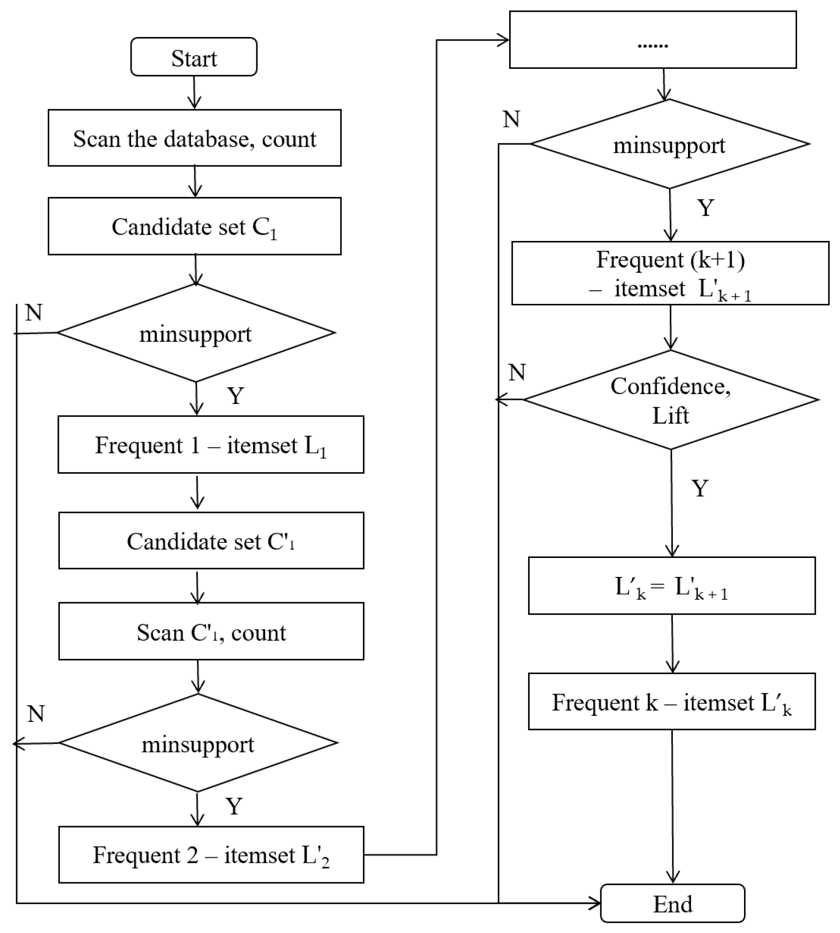
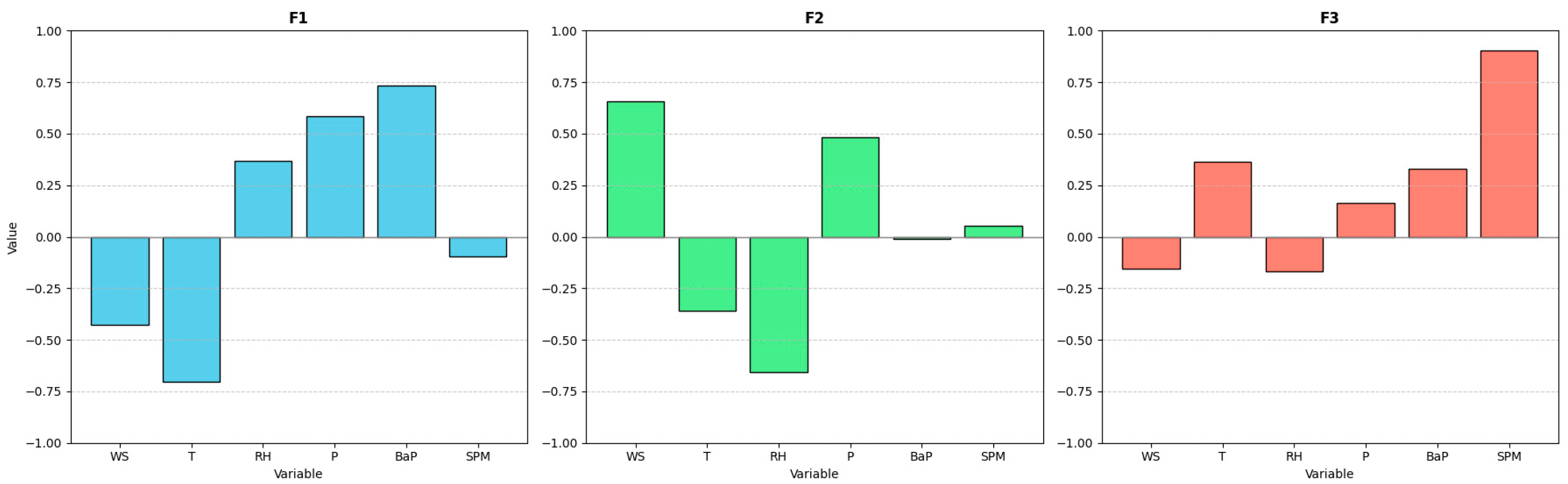
3.1. Feature Analysis

In 
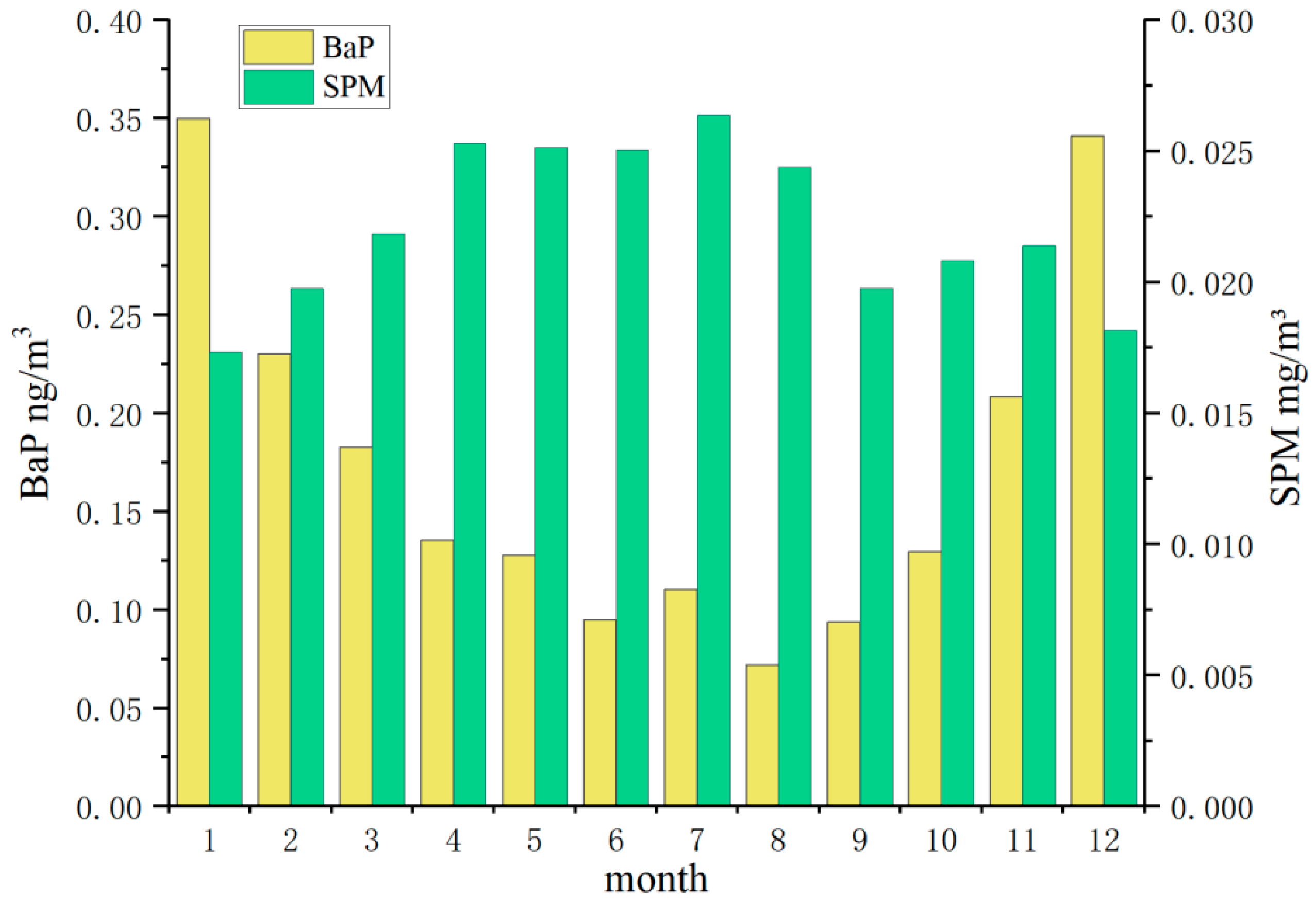
Figure 4, the overall monthly average of B(a)P was approximately twofold lower during the warm seasons (spring–summer: March–August) compared with that during the cold season (autumn–winter: September–February). From November to February, the monthly averages of B(a)P were relatively high, ranging from ~0.2 to 0.35 ng/m3. During summer, the lowest value was reported in August, ~0.07 ng/m3. This pronounced seasonal variation is primarily attributed to the enhanced atmospheric degradation of B(a)P during the warmer months, which is driven by two key mechanisms:
  • Photodegradation: Strong summer UV irradiation promotes B(a)P decomposition, as reflected by the significantly lower BaP/BeP ratio in warm seasons (0.66) compared with that in winter (1.08) [36]. To quantify this effect, a vapor-phase reaction model incorporating stepwise repartitioning was applied. This revealed that B(a)P’s atmospheric half-life decreases to 8 h under summer conditions (high OH radical concentration: 5 × 106 cm−3; 99% vapor-phase reaction), whereas it extends to 770 h in winter (low OH: 0.5 × 106 cm−3; 90–99% particle-bound) [37]. These results align with the observed August minimum (0.07 ng/m3) and explain B(a)P’s persistence in cold seasons.
  • Ozonolysis: Elevated ozone levels from spring to summer [38] further accelerate B(a)P degradation as its molecular structure is particularly vulnerable to ozone-induced oxidative cleavage. The synergy between photolysis and ozonolysis dominates over potential emission source variations, considering Kyoto’s reliance on electric heating in winter, which minimizes combustion-related B(a)P emissions.
In contrast to B(a)P, SPM exhibited an opposite seasonal trend, with higher monthly averages in warm seasons. This divergence arises from the following distinct physicochemical drivers:
  • Secondary aerosol formation: Active photochemical reactions in summer promote the oxidation of SO2 and NOx to sulfate and nitrate aerosols, significantly increasing the SPM mass.
  • Non-combustion contributions:
    • Biogenic secondary organic aerosols (SOA): Warm-season emissions of biogenic volatile organic compounds are oxidized to SOA, contributing to SPM.
    • Resuspended dust: Increased wind speeds and anthropogenic activities in spring/summer promote dust resuspension.
  • Regional transport: Prevailing wind patterns in Kyoto during warm seasons may import aerosols from industrial/urban areas.
  • Suppressed winter combustion sources: Unlike coal-dependent regions, Kyoto reduces its direct SPM emissions in winter through its electric heating practices, decoupling its seasonality from B(a)P.
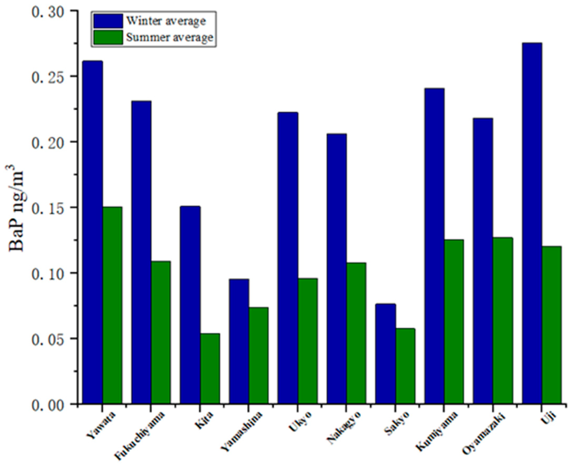
Figure 5 and Figure 6 show the seasonal variations in the B(a)P and SPM concentrations during warm and cold seasons across various regions, as detailed in Table A1 and Table A2 of Appendix A.2. The average B(a)P concentration was higher in the cold season than that in the warm season by ~1.3–3 times; similar results were reported in previous studies [39,40].
High B(a)P concentrations were observed because industrial parks in cities such as Yahata City and Fukuchiyama City generate high amounts of pollutants. These industrial parks are surrounded by abundant transportation hubs, and transportation logistics rely more on heavy-duty trucks that use diesel fuel. These factors are accompanied by unfavorable meteorological conditions such as atmospheric stability layers, low wind speed, or lack of precipitation during the cold season. In contrast, the average SPM was lower (by approximately half) in the cold season than in the warm season. The seasonal variations in B(a)P and SPM concentration were mainly due to differences in their sources and atmospheric behavior mechanisms. The seasonal variations in B(a)P were highly influenced by fuel combustion emissions and photochemical degradation, whereas those in SPM were influenced by secondary particulate matter generation and dust lifting.

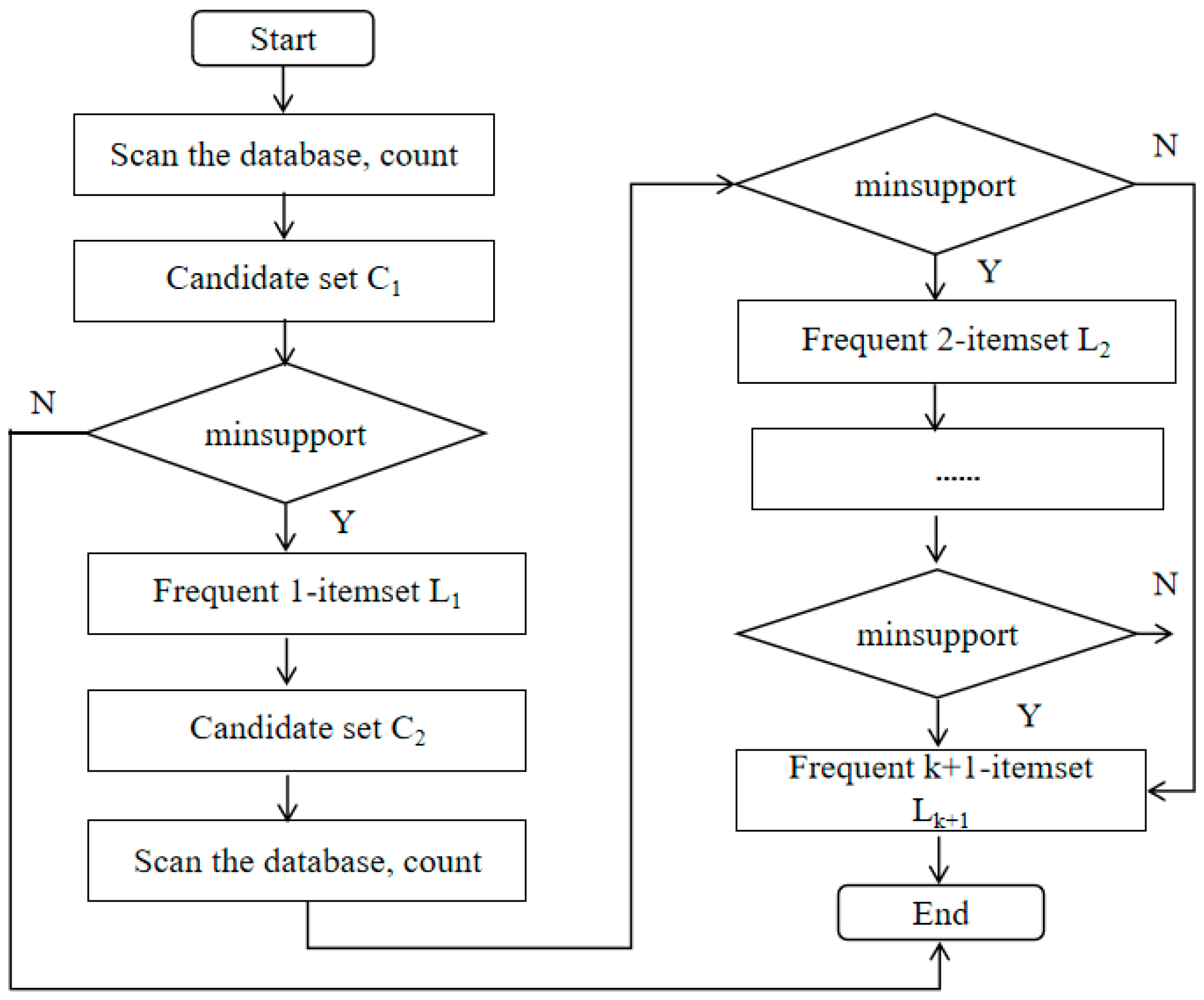
3.2. Association Relationships

The influence mechanism of SPM and meteorological factors over low, medium, and high B(a)P concentrations was determined based on 69 strong association rules. These rules were analyzed and arranged in an ascending order based on the dimensionality of influencing factors in the antecedent. A total of 58 strong association rules were mined at low B(a)P concentration (<0.185 ng/m3), spanning from one-dimensional to two-dimensional association rules. Table 3 shows the 1 one-dimensional association rule and 18 2D association rules.
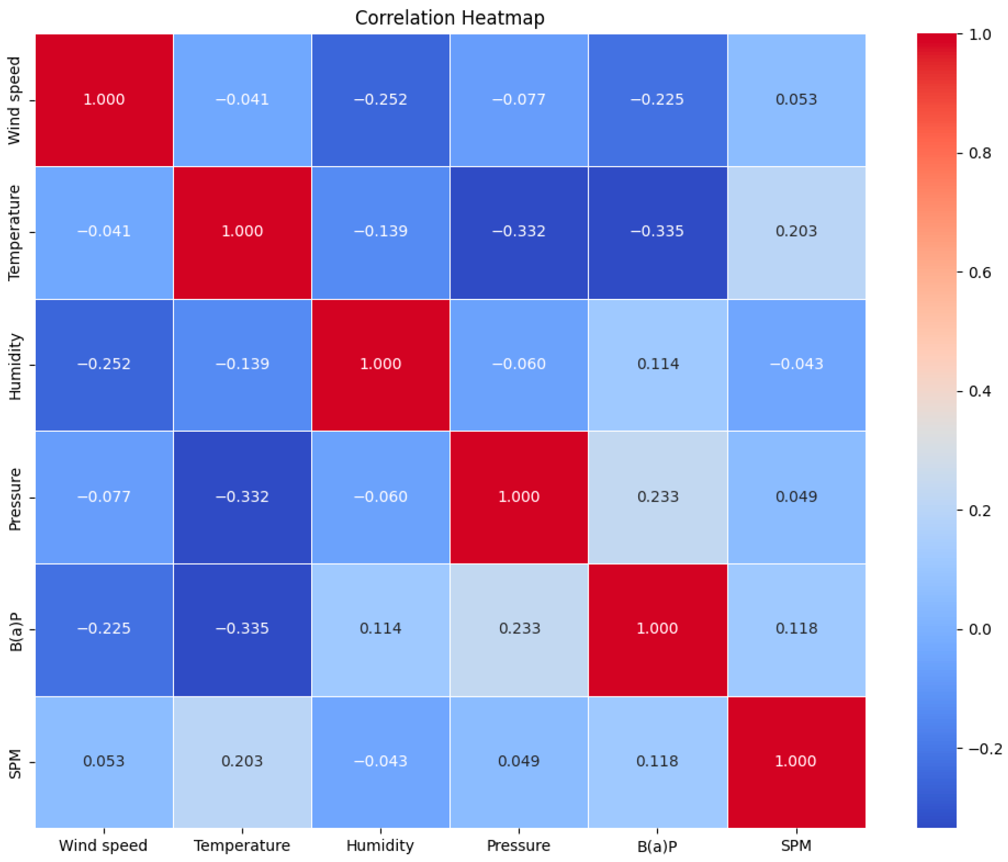
Numbers 0 and 4 indicate that adding humidity to high temperatures increases the confidence by 3%, suggesting that humidity considerably influences B(a)P concentrations for maintaining it at low levels. A comparison of numbers 8, 9, 16, and 19 reveals that rising temperatures increase the likelihood of B(a)P remaining at a low concentration by 7%. Numbers 11 and 12 show that higher pressure decreases the confidence by 3%, highlighting an inverse relationship. Numbers 17 and 18 indicate that as the wind speed increases, the confidence increases by 8%. These findings indicate that low humidity, low pressure, high wind speed, and high temperatures contribute to maintaining B(a)P at low concentrations.
In one-dimensional association rules, the probability of B(a)P being at a low concentration (B1) is 91.95% at high temperatures (T3). By integrating additional factors, this rule evolves into a 2D association rule. Excluding the influence of SPM and focusing solely on meteorological factors, numbers 1 and 4 reveal that transitioning from low pressure (P1) to high temperature (T3) reduces the confidence from 100% to 92.85% under low humidity (H1). This indicates that low pressure is more sensitive to B(a)P concentrations than high temperatures (P > T). A comparison of numbers 1 and 9 indicates that, at low pressure and when transitioning from low humidity to high temperature, confidence decreases from 100% to 93.42%; this suggests that humidity has higher sensitivity than temperature (H > T). A comparison of numbers 4 and 9 shows that at constant temperatures, confidence increases when transitioning from low humidity to low pressure. This further emphasizes that pressure is more influential than humidity (P > H). Therefore, the sensitivity ranking of meteorological factors is as follows: pressure > humidity > temperature.
A comparison of numbers 4, 5, 9, 11, 13, and 14 revealed that high wind speed consistently exhibits higher confidence than high temperature. Thus, temperature sensitivity was lower than wind speed sensitivity (T < WS). A comparison of numbers 1 and 11 under constant pressure conditions showed that low humidity demonstrated a 5% higher confidence than high wind speed, suggesting that humidity sensitivity exceeded wind speed sensitivity (WS < H). Based on these findings, the preliminary sensitivity ranking of meteorological factors is pressure > humidity > wind speed > temperature.
By transitioning to three-dimensional association rules, the conclusions drawn from the two-dimensional association rule mining are further compared in Table 4. By incorporating the influence of SPM into the association rules, phenomena contrary to those reported in Table 3 were observed. Analyzing the relationships captured in rules (23, 34, 40) and (29, 37) revealed that as humidity increased to the highest level and SPM remained at medium or high concentrations under high temperatures, the confidence decreased from 100% to 90.91% and 94.74%. This high humidity reduced the likelihood of B(a)P remaining at a low concentration. Similarly, when pressure was analyzed alongside SPM and temperature in rules 41 and 48, increasing pressure increased the confidence level from 96.15% to 100%. This trend contradicted the findings of the 2D association rules. This discrepancy can be attributed to the low SPM concentration in the air and high temperatures, which facilitated the volatilization, dispersion, and photochemical degradation of B(a)P.
A comparison of rule pairs (20, 21), (38, 39), (45, 46), and (55, 56) revealed that, with the other two factors held constant, an increase in wind speed increased the confidence by ~6% to −10%. This indicated that wind speed positively influenced the dispersion of B(a)P. A comparison of rules 51, 52, 54, and 56 indicated that the effect of temperature on B(a)P was consistent with the findings of 2D association rules. As the temperature increased, the confidence level increased by ~10%. By integrating the influence of SPM into the association rules, varying confidence levels were observed under different meteorological conditions, even when the B(a)P concentration was constant. A comparison of rules 33, 34, and 35 revealed that high SPM concentrations, high temperature, and moderate humidity gradually decreased the confidence levels. This observation indicated that meteorological conditions facilitated the dispersion of pollutants, thereby maintaining consistently low B(a)P concentrations. A different pattern was evident in rules 41 and 44, where low-pressure conditions combined with high temperatures indicated that B(a)P concentrations were affected by SPM concentrations.
The sensitivity of meteorological factors was evaluated using 3D association rules rather than the 2D association rules. Specifically, rules 19–21 along with rules 35 and 36 demonstrated that wind speed sensitivity surpassed that of temperature, with higher confidence levels of 7–10% (T < WS). Moreover, rules 37 and 53 indicated that pressure sensitivity exceeded humidity sensitivity, with confidence levels higher by ~5% (P > H). A comparison of rules 32 and 47 revealed that the confidence level for humidity was 97.56%, slightly higher than that for wind speed at 97.06%. This indicated that humidity sensitivity marginally surpassed wind speed sensitivity (WS < H). The findings from the 3D association rules are consistent with those from the 2D association rules, which confirmed the following sensitivity ranking: pressure > humidity > wind speed > temperature.
Empirical observations and meteorological mechanisms support the dominant role of atmospheric pressure in driving the correlations between PAHs and pollutants. Specifically, PAHs concentrations exhibit a highly significant positive correlation with atmospheric pressure compared with other meteorological parameters (e.g., r = 0.868, p < 0.01) [41]. This can be explained by contrasting pressure-driven dispersion patterns:
  • High-pressure systems suppress vertical dispersion through subsidence and diverging airflow, trapping pollutants locally and enhancing their adsorption onto particulate matter.
  • Conversely, low-pressure systems promote horizontal dispersion via rising air currents, leading to pollutant dilution [42].
Importantly, the sensitivity to pressure variations is most pronounced under the low-concentration B(a)P conditions in our study. This differential response highlights the critical regulatory role of pressure-driven suppression of atmospheric dispersion in governing the dynamics of low-concentration PAHs.
When the B(a)P concentration was at a low level (B1), the antecedents of the 3D association rules comprised all influencing factors, thereby rendering the further analysis of the four-dimensional association rules unnecessary.
At medium and high B(a)P concentrations (>0.185 ng/m3), two strong 2D, three 3D, and four 4D association rules were identified at the B2 level and two strong association rules were identified at the B3 level in Table 5, completely encompassing the complete set of influencing factors. Compared with the low B(a)P concentrations, these rules primarily highlight the meteorological conditions of increasing pressure, decreasing temperature, and decreasing wind speed. High pressure stabilizes the atmosphere, reduces pollutant dispersion, and causes pollutant accumulation in localized areas. Lower temperatures enhance air stability, decrease convection, and promote the deposition and accumulation of pollutants. Lower wind speeds weaken the diffusion of particulate matter, resulting in higher B(a)P concentrations in the air. Moreover, lower temperatures may enhance B(a)P adsorption, further increasing B(a)P concentrations.
A comparison of rules 22 and 23 in Table 4 with rule number 60 in Table 5 revealed that a decrease in the temperature from high to low corresponded to an increase in the B(a)P concentration level. This finding highlighted the inverse relationship between temperature and B(a)P concentration, suggesting that lower temperatures contributed to higher B(a)P concentration. A comparison of rule number 19 (Table 4) with rule number 63 (Table 5) revealed that adding the SPM (SP3) influence to the association rules increased B(a)P concentrations. The combination of these results and the phenomenon of lower B(a)P concentrations indicated that SPM exerted a certain effect on the B(a)P concentration.

3.3. Comparison of Methods

Figure 7 shows the correlation matrix of the PCA; temperature and wind speed exhibit a significant negative correlation with B(a)P concentration, indicating that low temperature and low wind speed may reduce the dispersion and dilution of pollutants, resulting in higher B(a)P concentrations. Atmospheric pressure has a moderate positive correlation with B(a)P concentration likely owing to pollutant accumulation under high-pressure conditions. Humidity has a weak positive correlation with B(a)P, potentially reflecting the influence of particle adsorption characteristics. Moreover, a strong association between B(a)P and SPM concentrations is observed. Table 6 shows the variance analysis of PCA. The eigenvalues C1 = 1.701, C2 = 1.226, and C3 = 1.132 and the cumulative variance contribution rate of the first three principal components reached 67.655%, covering most information. This indicated that the first three principal components in Table 7 represented the initial indicators for analysis. These three indicators were, therefore, denoted as F1, F2, and F3.
Table 7 shows the component matrix of PCA and Figure 8 shows the contribution of original variables to the three indicators, further revealing the relationship between B(a)P and the meteorological factors. The first component (F1; 28.346% of variance) exhibited a high positive loading for B(a)P (BaP = 0.732) along with negative loadings for temperature (T = −0.703) and wind speed (WS = −0.429), indicating that B(a)P concentrations tend to increase under low temperature and weak winds. The second and third components (F2 and F3) exhibited weak loadings for B(a)P (BaP = −0.010 and 0.328, respectively), indicating that other meteorological combinations had limited influence on variations in B(a)P concentrations.
The qualitative expression of results indicated that wind speed and temperature were negatively correlated with B(a)P, whereas humidity, pressure, and SPM were positively correlated with B(a)P. This conclusion essentially aligned with the findings obtained using association rule algorithms.

4. Conclusions

Herein, multidimensional analysis of association rules involving SPM, meteorological factors, and atmospheric pollutant B(a)P was performed to determine variations in B(a)P across different combinations of influencing factors. Contrasting sensitivities of various meteorological factors to B(a)P were quantitatively compared by analyzing changes in confidence levels that characterized the association relationships. The main findings were as follows:
(1) Herein, several methodological improvements were made. First, the K-means clustering method was used along with the “elbow method” using the SSE metric, which resulted in more reasonable clustering intervals. Second, the initial selection of the Apriori association rule mining algorithm demonstrated low computational efficiency, which resulted in disordered association rules. Through algorithm optimization, the processing efficiency was considerably improved, and by introducing the constraint parameter “lift” and eliminating invalid association rules, the optimized association rule results became more reliable and accurate.
(2) At low B(a)P concentrations, low humidity, low atmospheric pressure, high wind speeds, and high temperatures, the probability that B(a)P concentrations will remain low increased. When the effects of high SPM concentrations were incorporated into the association rule model, the accompanying favorable meteorological conditions accelerated pollutant dispersion, such that B(a)P concentrations remained low. In this case, SPM concentration has a positive effect on B(a)P concentrations. The sensitivity levels of meteorological factors, as verified via the combined analysis of 2D and 3D association rules, demonstrated the following ranking: pressure > humidity > wind speed > temperature.
(3) B(a)P concentration increases with increasing pressure, decreasing temperature, and decreasing wind speed. The change in humidity is relatively small; however, when B(a)P concentration is low, the confidence of the rule decreases as the humidity increases, indicating that high humidity may increase B(a)P concentration. However, at high B(a)P concentrations, due to the limitation of the number of rules, we failed to determine a clear meteorological factor sensitivity ranking. This may reflect the model’s limitations in capturing complex associations at high concentrations.
(4) To verify the significant factors influencing the variations in B(a)P concentration obtained via association algorithms, the data were subjected to PCA along with B(a)P concentration data. The results were generally consistent with the conclusions obtained from the association rule algorithm, indicating that the optimized Apriori algorithm exhibited high accuracy in association rule mining. Compared with traditional statistical methods, the association rule algorithm offers more detailed and nuanced insights. PCA primarily focuses on revealing linear correlations and principal components between variables, typically yielding only positive or negative correlations between two types of factors. In contrast, the association rule algorithm can mine complex, nonlinear associations among multiple factor combinations and quantify the impact of each factor on the results. The association rule algorithm provides more detailed conclusions than PCA. For instance, at low BaP concentrations, various meteorological conditions differently affect confidence levels and the impact of factor combinations on concentration levels is more intuitive.
Limitations and Future Directions: Despite its novel contributions, this study has several limitations. First, the use of monthly averaged data from a limited number of stations may obscure short-term pollution dynamics and spatial heterogeneity. Second, the lack of data on copollutants (e.g., O3 and NOx) that could interact with PAHs through photochemical pathways limits our accounting of photochemical interactions that may influence PAHs concentrations, potentially biasing our associations. Third, the probabilistic nature of association rules precludes precise dose–response quantification. Future work should address these gaps by integrating high-resolution monitoring (e.g., mobile sensor networks), mechanistic modeling, and advanced algorithms (e.g., FP-Growth and neural networks).

Author Contributions

M.W.: Conceptualization, Methodology, Formal analysis and investigation, Original draft writing. T.K.: Conceptualization, Methodology, Analysis, Resources, Supervision, Original draft reviewing and editing. All authors have read and agreed to the published version of the manuscript.

Funding

This research received no external funding.

Institutional Review Board Statement

Not applicable.

Informed Consent Statement

Not applicable.

Data Availability Statement

Environmental monitoring data can be obtained from the public platforms of the National Institute for Environmental Studies (NIES) (https://tenbou.nies.go.jp/) (accessed on 6 June 2024) and the Japan Meteorological Agency (JMA) (https://www.data.jma.go.jp/stats/etrn/index.php) (accessed on 6 June 2024). This includes continuous monitoring data of B(a)P, SPM, and meteorological factors from different regions.

Use of Artificial Intelligence

No AI or AI-assisted tools were used in drafting any aspect of this manuscript, including text generation, language editing, or data analysis. All content was prepared and reviewed solely by the authors.

Acknowledgments

We thank the reviewers and editors for their valuable comments.

Conflicts of Interest

The authors declare no conflicts of interest.

Abbreviations

The following abbreviations are used in this manuscript:
AIArtificial intelligence
CMAQCommunity multiscale air quality
JMAJapan Meteorological Agency
NIESNational Institute for Environmental Studies
GSIGeospatial Information Authority of Japan
PAHsPolycyclic aromatic hydrocarbons
PCAPrincipal component analysis
SPMSuspended particulate matter
SSESum of squared error

Appendix A

Appendix A.1. Data Discretization Theory

The K-means algorithm primarily comprises the following five steps:
(1) Determine the value of K’, which represents the number of groups to be partitioned, based on the users’ subjective setting.
(2) Randomly select a specified number of data points to serve as centroids.
(3) Calculate the distance from all data points to the closest centroid based on the Euclidean distance:
D C , X = i = 1 n ( c i x i ) 2 ,
where Ci denotes the centroid and xi denotes all data categories.
(4) Group the data with similar distances, calculated in step (3), into one cluster. Then, calculate their average within each cluster to obtain new centroid points.
(5) Repeat the process of calculating the mean to obtain the final centroid points for K’ clusters. Compare these final centroids with the centroids obtained in step (2). If there is no change in centroids, terminate the program; otherwise, continue with the calculations.
The SSE principle in K-means algorithm is as follows: According to step (5) of the K-means method, as K’ increases, the differences within each cluster decrease. This gradually minimizes the variance. When K’ is smaller than the true K, adjusting the K’ value reduces the differences within each group and SSE declines rapidly. Eventually, it reaches a point near the true K, where SSE shows a sudden change—this inflection point is of interest. Beyond this point, as K’ continues to increase, SSE stabilizes and does not decrease considerably. Thus, the appropriate number of clusters is generally indicated by the inflection point determined by the impact of K’ on the SSE. The main formulae are shown in (5), where a represents the data in each clustering group Ci and bi is the centroid of Ci.
S S E = i = 1 k a i a b i 2

Appendix A.2. Optimization of the Apriori Algorithm

The Apriori algorithm (prior criterion) was selected for mining frequent itemsets of Boolean data for association rule mining based on various data characteristics. This algorithm could effectively and rapidly mine association rules.
Figure A1. Apriori algorithm flowchart.
Air 03 00015 g0a1
Figure A1 shows the flowchart of Apriori algorithm that scans the database each time a frequent itemset is obtained. Consequently, the traditional Apriori algorithm is limited to handling datasets with few categories and small data volumes. In cases wherein numerous categories and large data volumes are involved, the disk performance of typical computers may not be able to manage the multiple database scans; this considerably reduces the computational efficiency. Therefore, the original algorithm structure must be optimized. To meet the minimum confidence criteria, the Apriori algorithm often unveils association rules that do not align with the actual research scenario when interpreting some strong association rules. For instance, in a dataset containing 100 entries, where the influencing factor X appears 60 times and the outcome Y appears 80 times as well as X and Y co-occurring 40 times, the probability of X and Y occurring together is 40%. Given the presence of X, the probability of Y occurring is 67%. Contrarily, without X, the probability of Y occurring is 80%. This suggests that the presence of X decreases the probability of Y, implying that X and Y are not associated. In addition to confidence, other metrics also need to be integrated.
Moreover, the association rules generated by the original algorithm cannot differentiate between antecedents and consequents. For instance, it may produce association rules in the format of “y → x, conf”. To enhance the specificity and accuracy of association rules, the antecedents must be denoted as SPM, and meteorological factors and consequents must be denoted as the atmospheric pollutant B(a)P within the algorithm. Based on the mechanism of association rules, low-dimensional and high-dimensional association rules must be compared (where low-dimensional and high-dimensional represent the process from a single antecedent to multiple antecedents). For instance, based on consistent confidence and lift, interpreting low-dimensional association rules can reveal patterns that align with real-world scenarios. Upon adding additional influencing factors, the rules transition to high-dimensional rules without changes in the consequents, confidence, and lift. In such cases, the excessive connections in high-dimensional association rules signify invalid rules, thereby necessitating optimization in rule filtering within the algorithm.
The original Apriori algorithm is optimized as follows:
(1) Load the dataset TID1…n after discretization, where data are referred to as an element (input items include the concentration of B(a)P, SPM concentration, and various types of discretized meteorological data), and stored as Database D.
(2) Scan and count each element item in Database D and store them as the candidate set C1. Compare the predefined minimum support level and prune the elements of the candidate set C1, retaining those greater than the minimum support level, to obtain the frequent itemset L1.
(3) Connect the frequent itemset L1 and store it as the candidate set C’1. Scan and count the elements in dataset C’1 to obtain candidate set C’2 and prune C’2 to obtain the frequent 2 itemset L’2.
(4) Repeat the pruning and connection operations downward until the final frequent (K + 1) itemset L’k+1 is found.
(5) Filter rules based on the optimized metrics and output strong association rules.
Table A1. Maximum, minimum, and average B(a)P concentrations in spring–summer and fall–winter (ng/m3).
Spring–SummerFall–Winter
B(a)PMaxMinAverageMaxMinAverage
Yawata10.00610.1511.50.0160.262
Fukuchiyama0.480.0090.1090.830.0130.232
Kita0.190.00720.0541.10.0160.151
Yamashina0.220.0130.0740.460.0080.096
Ukyo0.450.0250.0960.690.0020.223
Nakagyo0.480.0050.1081.50.0060.206
Sakyo0.260.00940.0580.330.00250.077
Kumiyama1.30.00340.1261.60.0170.241
Oyamazaki 0.740.00380.1271.80.0210.218
Uji0.460.0180.1211.10.0390.276
Citywide1.30.00340.1201.80.0020.226
Table A2. Maximum, minimum, and average SPM concentrations in spring–summer and fall–winter (mg/m3).
Spring–SummerFall–Winter
SPMMaxMinAverageMaxMinAverage
Yawata0.0460.0110.0240.0390.0070.019
Fukuchiyama0.04300.0250.0330.0090.018
Kita0.0220.0110.0150.0120.0060.009
Yamashina0.0240.0140.0160.0150.010.012
Ukyo0.0390.0170.0280.0270.0160.020
Nakagyo0.050.0120.0270.0410.0080.022
Sakyo0.0230.0110.0140.0130.0070.010
Kumiyama0.0350.0110.0220.0280.0090.018
Oyamazaki0.0540.010.0280.0510.0080.022
Uji0.0420.0180.0270.030.0120.022
Citywide0.05400.0250.0510.0060.020

References

  1. Ravindra, K.; Wauters, E.; Van Grieken, R. Variation in particulate PAHs levels and their relation with the transboundary movement of the air masses. Sci. Total Environ. 2008, 396, 100–110. [Google Scholar] [CrossRef] [PubMed]
  2. Kim, K.-H.; Jahan, S.A.; Kabir, E.; Brown, R.J. A review of airborne polycyclic aromatic hydrocarbons (PAHs) and their human health effects. Environ. Int. 2013, 60, 71–80. [Google Scholar] [CrossRef] [PubMed]
  3. Olsson, A.C.; Fevotte, J.; Fletcher, T.; Cassidy, A.; Mannetje, A.t.; Zaridze, D.; Szeszenia-Dabrowska, N.; Rudnai, P.; Lissowska, J.; Fabianova, E. Occupational exposure to polycyclic aromatic hydrocarbons and lung cancer risk: A multicenter study in Europe. Occup. Environ. Med. 2010, 67, 98–103. [Google Scholar] [CrossRef]
  4. Diggs, D.L.; Huderson, A.C.; Harris, K.L.; Myers, J.N.; Banks, L.D.; Rekhadevi, P.V.; Niaz, M.S.; Ramesh, A. Polycyclic aromatic hydrocarbons and digestive tract cancers: A perspective. J. Environ. Sci. Health Part C 2011, 29, 324–357. [Google Scholar] [CrossRef]
  5. Boström, C.-E.; Gerde, P.; Hanberg, A.; Jernström, B.; Johansson, C.; Kyrklund, T.; Rannug, A.; Törnqvist, M.; Victorin, K.; Westerholm, R. Cancer risk assessment, indicators, and guidelines for polycyclic aromatic hydrocarbons in the ambient air. Environ. Health Perspect. 2002, 110, 451–488. [Google Scholar] [CrossRef]
  6. Hůnová, I.; Kurfürst, P.; Vlasáková, L.; Schreiberová, M.; Škáchová, H. Atmospheric Deposition of Benzo [a] pyrene: Developing a Spatial Pattern at a National Scale. Atmosphere 2022, 13, 712. [Google Scholar] [CrossRef]
  7. Roy, R.; Jan, R.; Gunjal, G.; Bhor, R.; Pai, K.; Satsangi, P.G. Particulate matter bound polycyclic aromatic hydrocarbons: Toxicity and health risk assessment of exposed inhabitants. Atmos. Environ. 2019, 210, 47–57. [Google Scholar] [CrossRef]
  8. Peterson, D.A.; Hyer, E.J.; Han, S.-O.; Crawford, J.H.; Park, R.J.; Holz, R.; Kuehn, R.E.; Eloranta, E.; Knote, C.; Jordan, C.E. Meteorology influencing springtime air quality, pollution transport, and visibility in Korea. Elem. Sci. Anthr. 2019, 7, 57. [Google Scholar] [CrossRef]
  9. Li, F.; Wang, H.; Wang, X.; Xue, Z.; Duan, L.; Kou, Y.; Zhang, Y.; Chen, X. Pollution characteristics of atmospheric carbonyls in urban Linfen in winter. Atmosphere 2020, 11, 685. [Google Scholar] [CrossRef]
  10. Lotrecchianoa, N.; Sofiaa, D.; Giulianoa, A.; Barlettaa, D.; Polettoa, M. Real-time on-road monitoring network of air quality. Chem. Eng. 2019, 74, 241–246. [Google Scholar] [CrossRef]
  11. Guo, Q.; Wu, D.; Yu, C.; Wang, T.; Ji, M.; Wang, X. Impacts of meteorological parameters on the occurrence of air pollution episodes in the Sichuan basin. J. Environ. Sci. 2022, 114, 308–321. [Google Scholar] [CrossRef]
  12. Erener, A.; Sarp, G.; Yıldırım, Ö. Seasonal air pollution investigation and relation analysis of air pollution parameters to meteorological data (Kocaeli/Turkey). In Advances in Remote Sensing and Geo Informatics Applications: Proceedings of the 1st Springer Conference of the Arabian Journal of Geosciences (CAJG-1), Tunisia 2018; Springer Nature: Berlin/Heidelberg, Germany, 2019; pp. 355–358. [Google Scholar]
  13. Demir, S.; Saral, A.; Ertürk, F.; Kuzu, L. Combined use of principal component analysis (PCA) and chemical mass balance (CMB) for source identification and source apportionment in air pollution modeling studies. Water Air Soil. Pollut. 2010, 212, 429–439. [Google Scholar] [CrossRef]
  14. Hao, Y. Numerical simulation of regional air pollution characteristics based on meteorological factors and improved Elman neural network algorithm. Appl. Nanosci. 2023, 13, 3383–3391. [Google Scholar] [CrossRef]
  15. Vidnerová, P.; Neruda, R. Air pollution modelling by machine learning methods. Modelling 2021, 2, 659–674. [Google Scholar] [CrossRef]
  16. Yuan, X.; Song, J.; Zeng, N.; Guo, J.; Ma, H. Correlation analysis and application investigation of multi-angle simultaneous polarization measurement data and concentration of suspended particulate matter in the atmosphere. Front. Environ. Sci. 2022, 10, 1031863. [Google Scholar] [CrossRef]
  17. Rushingabigwi, G.; Nsengiyumva, P.; Sibomana, L.; Twizere, C.; Kalisa, W. Analysis of the atmospheric dust in Africa: The breathable dust’s fine particulate matter PM2. 5 in correlation with carbon monoxide. Atmos. Environ. 2020, 224, 117319. [Google Scholar] [CrossRef]
  18. Di Bernardino, A.; Iannarelli, A.M.; Casadio, S.; Perrino, C.; Barnaba, F.; Tofful, L.; Campanelli, M.; Di Liberto, L.; Mevi, G.; Siani, A.M. Impact of synoptic meteorological conditions on air quality in three different case studies in Rome, Italy. Atmos. Pollut. Res. 2021, 12, 76–88. [Google Scholar] [CrossRef]
  19. Nguyen, G.T.H.; Shimadera, H.; Uranishi, K.; Matsuo, T.; Kondo, A.; Thepanondh, S. Numerical assessment of PM2.5 and O3 air quality in continental Southeast Asia: Baseline simulation and aerosol direct effects investigation. Atmos. Environ. 2019, 219, 117054. [Google Scholar] [CrossRef]
  20. Che, W.; Zheng, J.; Wang, S.; Zhong, L.; Lau, A. Assessment of motor vehicle emission control policies using Model-3/CMAQ model for the Pearl River Delta region, China. Atmos. Environ. 2011, 45, 1740–1751. [Google Scholar] [CrossRef]
  21. Seaman, N.L. Meteorological modeling for air-quality assessments. Atmos. Environ. 2000, 34, 2231–2259. [Google Scholar] [CrossRef]
  22. Badas, M.G.; Salvadori, L.; Garau, M.; Querzoli, G.; Ferrari, S. Urban areas parameterisation for CFD simulation and cities air quality analysis. Int. J. Environ. Pollut. 2019, 66, 5–18. [Google Scholar] [CrossRef]
  23. Karatzas, K.D.; Kaltsatos, S. Air pollution modelling with the aid of computational intelligence methods in Thessaloniki, Greece. Simul. Model. Pract. Theory 2007, 15, 1310–1319. [Google Scholar] [CrossRef]
  24. Sfetsos, A.; Vlachogiannis, D. A new approach to discovering the causal relationship between meteorological patterns and PM10 exceedances. Atmos. Res. 2010, 98, 500–511. [Google Scholar] [CrossRef]
  25. Shahriar, S.A.; Kayes, I.; Hasan, K.; Salam, M.A.; Chowdhury, S. Applicability of machine learning in modeling of atmospheric particle pollution in Bangladesh. Air Qual. Atmos. Health 2020, 13, 1247–1256. [Google Scholar] [CrossRef] [PubMed]
  26. Zhang, Y.; Wang, D.; Wu, Y.; Liu, Y.; Zhang, N.; Li, Y. Network intrusion detection based on apriori-kmeans algorithm. In 3D Imaging—Multidimensional Signal Processing and Deep Learning: 3D Images, Graphics and Information Technologies, Volume 1; Jain, L.C., Kountchev, R., Tai, Y., Kountcheva, R., Eds.; Springer Nature: Singapore, 2022; pp. 101–109. [Google Scholar]
  27. Sherkat, E.; Velcin, J.; Milios, E.E. Fast and simple deterministic seeding of KMeans for text document clustering. In Proceedings of the Experimental IR Meets Multilinguality, Multimodality, and Interaction: 9th International Conference of the CLEF Association, CLEF 2018, Avignon, France, 10–14 September 2018; pp. 76–88. [Google Scholar]
  28. Lang, X.; Zhao, Z.; Xiong, G. The Analysis of Traffic Drivers’ Behavior based on Kmeans. In Proceedings of the 2017 International Conference on Computer Science and Artificial Intelligence, Jakarta, Indonesia, 5–7 December 2017; pp. 232–236. [Google Scholar]
  29. Huo, Y.; Cao, Y.; Wang, Z.; Yan, Y.; Ge, Z.; Yang, Y. Traffic anomaly detection method based on improved GRU and EFMS-Kmeans clustering. Comput. Model. Eng. Sci. 2021, 126, 1053–1091. [Google Scholar] [CrossRef]
  30. Tao, Y.; Deng, J.; Song, X. Drug audit based on bisecting k-means clustering algorithm. In Proceedings of the 2019 International Conference on Cyber-Enabled Distributed Computing and Knowledge Discovery (CyberC), Guilin, China, 17–19 October 2019; pp. 265–270. [Google Scholar]
  31. Wang, C.; Zheng, X. Application of improved time series Apriori algorithm by frequent itemsets in association rule data mining based on temporal constraint. Evol. Intell. 2020, 13, 39–49. [Google Scholar] [CrossRef]
  32. Shabtay, L.; Fournier-Viger, P.; Yaari, R.; Dattner, I. A guided FP-Growth algorithm for mining multitude-targeted item-sets and class association rules in imbalanced data. Inf. Sci. 2021, 553, 353–375. [Google Scholar] [CrossRef]
  33. Chen, J.; Song, X.; Zang, L.; Mao, F.; Yin, J.; Zhang, Y. Spatio-temporal association mining of intercity PM2. 5 pollution: Hubei Province in China as an example. Environ. Sci. Pollut. Res. 2023, 30, 7256–7269. [Google Scholar] [CrossRef]
  34. Araneda, O.F.; Cavada, G. Atmospheric pollutants affect physical performance: A natural experiment in horse racing studied by principal component analysis. Biology 2022, 11, 687. [Google Scholar] [CrossRef]
  35. Onat, B.; Şahin, Ü.A.; Bayat, C. Assessment of particulate matter in the urban atmosphere: Size distribution, metal composition and source characterization using principal component analysis. J. Environ. Monit. 2012, 14, 1400–1409. [Google Scholar] [CrossRef]
  36. Okuda, T.; Kumata, H.; Naraoka, H.; Takada, H. Origin of atmospheric polycyclic aromatic hydrocarbons (PAHs) in Chinese cities solved by compound-specific stable carbon isotopic analyses. Org. Geochem. 2002, 33, 1737–1745. [Google Scholar] [CrossRef]
  37. Harrison, R.M.; Jang, E.; Alam, M.S.; Dang, J. Mechanisms of reactivity of benzo (a) pyrene and other PAH inferred from field measurements. Atmos. Pollut. Res. 2018, 9, 1214–1220. [Google Scholar] [CrossRef]
  38. Keyte, I.J.; Harrison, R.M.; Lammel, G. Chemical reactivity and long-range transport potential of polycyclic aromatic hydrocarbons–a review. Chem. Soc. Rev. 2013, 42, 9333–9391. [Google Scholar] [CrossRef] [PubMed]
  39. Gianelle, V.; Colombi, C.; Caserini, S.; Ozgen, S.; Galante, S.; Marongiu, A.; Lanzani, G. Benzo (a) pyrene air concentrations and emission inventory in Lombardy region, Italy. Atmos. Pollut. Res. 2013, 4, 257–266. [Google Scholar] [CrossRef]
  40. Barrado, A.I.; García, S.; Barrado, E.; Pérez, R.M. PM2. 5-bound PAHs and hydroxy-PAHs in atmospheric aerosol samples: Correlations with season and with physical and chemical factors. Atmos. Environ. 2012, 49, 224–232. [Google Scholar] [CrossRef]
  41. Wang, P.-C.; Yang, L.-X.; Bie, S.-J.; Huang, Q.; Qi, A.-A.; Tuo, X.; Wang, Y.-M.; Xu, P.; Zhang, T.-Q.; Wang, W.-X. Pollution Characteristics and Source Analysis of Atmospheric PM 2.5-bound Polycyclic Aromatic Hydrocarbons in a Port Area. Huan Jing Ke Xue Huanjing Kexue 2022, 43, 4458–4466. [Google Scholar] [CrossRef]
  42. Elorduy, I.; Elcoroaristizabal, S.; Durana, N.; García, J.; Alonso, L. Diurnal variation of particle-bound PAHs in an urban area of Spain using TD-GC/MS: Influence of meteorological parameters and emission sources. Atmos. Environ. 2016, 138, 87–98. [Google Scholar] [CrossRef]
Figure 1. Administrative boundaries and geographic distribution of cities and towns in Kyoto Prefecture, Japan.
Air 03 00015 g001
Figure 2. Cluster K value elbow plot for each factor.
Air 03 00015 g002
Figure 3. Flowchart of the algorithm after optimization.
Air 03 00015 g003
Figure 4. Mean concentrations of B(a)P and SPM by month.
Air 03 00015 g004
Figure 5. Mean B(a)P concentrations by season.
Air 03 00015 g005
Figure 6. Mean SPM concentrations by season.
Air 03 00015 g006
Figure 7. Correlation matrix for principal component analysis (PCA).
Air 03 00015 g007
Figure 8. Contribution of the original variables to the composition of three new variables in principle component analysis.
Air 03 00015 g008
Table 1. Data levels.
DataClass 1Class 2Class 3
B(a)P (ng/m3)B1 ≤ 0.1850.185 < B2 ≤ 0.4380.438 < B3 ≤ 1.075
SPM (mg/m3)SP1 ≤ 0.0190.019 < SP2 ≤ 0.0280.028 < SP3 ≤ 0.043
Wind speed(m/s)WS ≤ 22 < WS2 ≤ 2.82.8 < WS3
Temperature (°C)T1 ≤ 12.312.3 < T2 ≤ 22.322.3 < T3
Humidity (%)H1 ≤ 5858 < H2 ≤ 6969 < H3
Pressure (hPa)P1 ≤ 1009.21009.2 < P2 ≤ 1022.31022.3 < P3
Table 2. Data transaction itemset.
B(a)PSPMWind SpeedPressureTemperatureHumidity
1B1SP2WS1P2T2H2
2B1SP1WS1P2T2H2
252B3SP2WS3P3T2H1
Table 3. Data transaction itemset: one- and two-dimensional strong association rules for SPM, meteorological factors, and low B(a)P concentrations.
NumberAntecedentSubsequentConfidence (%)
0‘T3’ ‘B1’91.95
1‘H1’‘P1’‘B1’100.00
2‘H1’‘SP1’‘B1’100.00
3‘H1’‘SP2’‘B1’92.30
4‘H1’‘T3’‘B1’92.85
5‘H1’‘WS2’‘B1’95.00
6‘H2’‘WS3’‘B1’93.75
7‘P1’‘SP1’‘B1’93.02
8‘P1’‘T1’‘B1’100.00
9‘P1’‘T3’‘B1’93.42
10‘P1’‘WS1’‘B1’94.12
11‘P1’‘WS3’‘B1’95.24
12‘P2’‘WS3’‘B1’92.86
13‘SP1’‘T3’‘B1’96.77
14‘SP1’‘WS3’‘B1’100.00
15‘SP2’‘T3’‘B1’93.55
16‘T1’‘WS3’‘B1’93.33
17‘T3’‘WS1’‘B1’92.68
18‘T3’‘WS3’‘B1’100.00
Table 4. Three-dimensional strong association rules for SPM, meteorological factors, and low B(a)P concentrations.
NumberAntecedentSubsequentConfidence (%)
19‘H1’‘P2’‘T2’‘B1’90.91
20‘H1’‘P2’‘WS2’‘B1’90.00
21‘H1’‘P2’‘WS3’‘B1’100.00
22‘H1’‘SP2’‘T2’‘B1’100.00
23‘H1’‘SP2’‘T3’‘B1’100.00
24‘H1’‘SP2’‘WS1’‘B1’100.00
25‘H1’‘SP2’‘WS3’‘B1’100.00
26‘H1’‘SP3’‘WS2’‘B1’100.00
27‘H1’‘T1’‘WS1’‘B1’100.00
28‘H1’‘T1’‘WS3’‘B1’100.00
29‘H1’‘T3’‘WS2’‘B1’100.00
30‘H2’‘P1’‘SP1’‘B1’90.00
31‘H2’‘P1’‘SP3’‘B1’90.00
32‘H2’‘P1’‘T3’‘B1’97.56
33‘H2’‘SP1’‘T3’‘B1’100.00
34‘H2’‘SP2’‘T3’‘B1’93.33
35‘H2’‘SP3’‘T3’‘B1’93.75
36‘H2’‘SP3’‘WS3’‘B1’100.00
37‘H2’‘T3’‘WS2’‘B1’94.74
38‘H3’‘P1’‘WS1’‘B1’94.44
39‘H3’‘P1’‘WS3’‘B1’100.00
40‘H3’‘SP2’‘T3’‘B1’90.91
41‘P1’‘SP1’‘T3’‘B1’96.15
42‘P1’‘SP1’‘WS1’‘B1’92.31
43‘P1’‘SP1’‘WS2’‘B1’92.00
44‘P1’‘SP3’‘T3’‘B1’91.30
45‘P1’‘SP3’‘WS1’‘B1’92.86
46‘P1’‘SP3’‘WS3’‘B1’100.00
47‘P1’‘T3’‘WS1’‘B1’97.06
48‘P2’‘SP1’‘T3’‘B1’100.00
49‘P2’‘SP2’‘T3’‘B1’100.00
50‘P2’‘SP3’‘WS3’‘B1’100.00
51‘P2’‘T1’‘WS3’‘B1’90.91
52‘P2’‘T2’‘WS3’‘B1’100.00
53‘P2’‘T3’‘WS2’‘B1’100.00
54‘SP1’‘T2’‘WS2’‘B1’91.67
55‘SP1’‘T3’‘WS1’‘B1’94.12
56‘SP1’‘T3’‘WS2’‘B1’100.00
57‘SP2’‘T3’‘WS1’‘B1’100.00
Table 5. Different dimensional strong association rules for SPM, meteorological factors, and medium and high B(a)P concentrations.
NumberAntecedentSubsequentConfidence (%)
58‘H2’‘P3’ ‘B2’100.00
59‘P3’‘WS1’ ‘B2’100.00
60‘H1’‘SP2’‘T1’ ‘B2’100.00
61‘H3’‘P2’‘SP3’ ‘B2’100.00
62‘H3’‘SP3’‘T1’ ‘B2’100.00
63‘H1’‘P2’‘SP3’‘T2’‘B2’100.00
64‘H1’‘SP3’‘T2’‘WS1’‘B2’100.00
65‘H2’‘SP2’‘T2’‘WS1’‘B2’100.00
66‘H3’‘SP3’‘T2’‘WS1’‘B2’100.00
67‘H1’‘P2’‘T1’‘WS1’‘B3’100.00
68‘H2’‘SP3’‘T1’‘WS1’‘B3’100.00
Table 6. Total ANOVA of PCA.
Total Variance Explained
Initial EigenvalueExtract the Sum of the Squares of the Loads
ComponentTotalPercentage VarianceCumulative%TotalPercentage VarianceCumulative%
11.70128.34628.3461.70128.34628.346
21.22620.43548.7821.22620.43548.782
31.13218.87367.6551.13218.87367.655
40.82713.78081.435
50.69911.64993.084
60.4156.916100.000
Table 7. Component matrix for principal component analysis.
Component Matrix
Component
F1F2F3
Wind speed (WS)−0.4290.657−0.156
Temperature (T)−0.703−0.3610.364
Humidity (RH)0.369−0.655−0.168
Pressure (P)0.5860.4820.164
B(a)P (BaP)0.732−0.0100.328
SPM (SPM)−0.0940.0540.902
Disclaimer/Publisher’s Note: The statements, opinions and data contained in all publications are solely those of the individual author(s) and contributor(s) and not of MDPI and/or the editor(s). MDPI and/or the editor(s) disclaim responsibility for any injury to people or property resulting from any ideas, methods, instructions or products referred to in the content.

